TSD

000493

---

NATURAL

TECHNICAL

TECHNOLOGY

MEMORANDUM

www,naturalrt.corn

Date:

April

3,

2009

Subject:

Groundwater

Modeling

of

Hutsonville

Pond

D

From:

Introduction

This

technical

memorandum

describes

results

of

modeling performed

to

evaluate

fate

and transport

in

the

upper

migration zone

at

the

Hulsonville Power

Station.

The

power

station

is

located

in

Crawford

County

Illinois, north

of

the

City

of Hutsonville

(Figure

1).

Modeling

was performed

in 2000

and 2005;

however,

the

results

were

reported

separately

and,

as

a

result,

were

difficult to follow

and

comprehend.

This

technical

memorandum

is

a

stand-alone document

that

fully

describes

model

development

and

reports

on

results

that

are relevant to

current

conditions and

closure

of

Pond

D.

Specifically,

the

model

was

used

to

provide

the

following informalion:

•

The

southward extent

to which off-site

concentrations

exceeded

Illinois

Class

1

Groundwater

Quality

Standards;

•

The reduction

in

boron

loading

to

the

Wabash

River

as

a

result

ofdewatering

and

closure

of

Pond

D;

•

The

effectiveness

of

the

proposed

remedial

strategy

for Pond

D

(consisting

of

a synthetic

cap

coupled

and

a

groundwater

collection

trench

along

the south

property

boundary);

and

•

The

volume of

groundwater

that

will

discharge

to

the

groundwater

collection

trench.

Transport

of boron

was

modeled

because

it

is

an

indicator

parameter

for

coal

ash

leachate,

it

is

mobile

in

groundwater,

and

its

concentration

in

downgradieni

monitoring

wells

is

nearly

an order of

magnitude

higher

than

its

Class

I

groundwater

quality

standard,

Three model

codes

were

used to

simulate

groundwater

flow

and

contaminant

transport:

'•

Leachate

percolation

after

pond

closure

was

modeled

using

the

Hydrologic

Evaluation

of

Landfill

Performance

(HELP)

model;

TCCHMEMO

-

MODF.L IXK-

1

NATURAL

RESOURCE

TECHNOLOGY

TSD

000494

---

TECHNICAL MEMORANDUM

•

Groundwater

flow

was

modeled

in

three

dimensions

using

MODFLOW

(The

HELP

model

provided

post-closure

leachale

percolation

rates

for

input

to

MODFLOW); and

•

Contaminant transport

was

modeled

in

three dimensions

using

MT3DMS

(MODFLOW

calculated

the

flow

field

that

MT3DMS used

in

the

contaminant

transport calculations).

Conceptual

Model

Hydrostratigraphy,

developed

from

site

boring

logs,

indicates

that the

upland

area near

Pond

D

consists

of

sand and

gravel

of

varying

thickness,

typically

10

to

20

feel,

underlain

by

15

to

more

than

30

feet

of

sandstone—this

is

referred to

as

the

upper

migration

zone

(Figure

2,

Cross

Section

A-A').

The

upper

sand

appears

lo

grade

to

a

fine-grained

silty

clay

toward

the

northern

portion

of

the

site

(Figure

2,

Cross

Section

C-C').

A

thick

shale unit underlies

the

sandstone at

an approximate

elevation

of

about

415

to

420

feet.

The Wabash River

valley

contains

a relatively

fine-grained

alluvium

from

land

surface to

an

elevation

of

about

410

to

415

feet,

underlain

by

sand

and

gravel

to

an

elevation

of

about

350

feet—the

sand and

gravel

at

depth

in

the Wabash river

valley

is

referred

to as

the

deep

alluvial

aquifer.

The

conceptual

model

for

this

site

is schematically

illustrated

below

and

as

follows:

There

are

three

sources

of

water:

natural

recharge

within

the

model

domain,

percolation

water

from

Pond

D,

and

groundwaier

flow

from

the

wesl.

Groundwater

in

the

upper

migration

zone

flows

horizontally

east,

discharging

into

the

Wabash

River,

a

regional

groundwater

sink.

Where coal

ash

is

encountered

within

the

upper

migration

zone,

groundwater

flows

horizontally through

the

ash.

Percolation

through

the

coal

ash and

groundwater

flow

through

ash

at

elevations below

the

water

table

are

the

sources

of

solute

mass

to the

model,

and

the

sink

for

solute

mass

is

the

Wabash

River.

(TECH

MEMO

-

MOOEL.DOC]

NATURAL

RESOURCE

TECHNOLOGY

TSD

000495

---

TECHNICAL

HELP

Modeling

The

Hydrologic

Evaluation

of

Landfill

Performance

(HELP)

code

was

developed

by

the

U.S.

Environmental

Protection

Agency

and

is

used

extensively

in

waste

facility

assessments.

HELP

predicts

one-dimensional

vertical

percolation

from

a

landfill

or

soil

column

based

on

precipitation,

evapotranspiration,

runoff,

and

the

geometry

and

hydrogeologic

properties

of

a layered

soil

and

waste

profile.

HELP

(Version

3.07;

Schroeder

et.

al,

1994)

was

used

to

estimate

percolation

from

Pond

D

during

dewatering and after

construction of

the

synthetic

cap.

The

hydrologic

data

required

by

and

entered into

HELP

are

listed

in

Table

1

and

described

in

the

following

paragraphs.

Help

Model

Approach

The

time

line for the

HELP

modeling

is

as

follows:

Dewatering

was

simulated

for

a

three

year

period,

then

the

cap

was

simulated

for

22

years.

The

22-year

cap

simulation

period

was

sufficient

for

the

system

to

reach

equilibrium.

Input

Data

Climatic

input

variables

were

synthetically

generated

by the

model

using

modified

default

values

for

Evansville,

Indiana,

and

a

latitude

of

39.13°

N

for

the

Hutsonville

Power

Station.

Rainfall

frequency

and

temperature

patterns

for

more

than

100

cities

are

programmed

into

HELP.

Evansville

was

selected

as

the

closest

city

to

Hutsonville.

The

model used Evansville's

precipitation

and

temperature

patterns

with

average

monthly precipitation

data

recorded

at

the

two

closest

monitoring

stations with

long-term

records'

to

generate

daily

precipitation

and

temperature data.

Modeling

was

performed

assuming

fair

vegetation,

which

generally

results

in

greater

infiltration

than

good

vegetation

and

is

therefore

conservative.

Physical

input

data

were

based

on

a

combination

of

measured

and

assumed

soil properties.

The ash

was

subdivided

into

three 60-inch

thick

sublayers.

This

subdivision

resulted

in

more

rapid percolation

responses

to

surface

changes,

such

as

dewatering,

than

two

90-inch

layers,

yet

provided

the

same

results

as

six 30-inch

thick layers.

The

15-foot combined

thickness

of

the ash

layers

represented

the

estimated

thickness

of

ash

above

the

water

table

after

dewatering.

[TECHMEMO-MODEL.DOC]

3

NATURAL

RESOURCE

TECHNOLOGY

TSD

000496

---

TECHNICAL MEMORANDUM

Hydrogeologic

properties

for

the

ash

and

cap

soils

were

selected

from

the

HELP

database.

Initial

moisture content

was

set

equal

to

its

porosity,

representing

ponded

conditions

immediately

prior

to

dewatering.

The

cap

scenario

was

simulated

with

initial

moisture

content

of

the

ash

layers

equal

to

the

moisture

content

calculated

by

HELP

at

the

end

of

the

dewatering

period.

Initial

moisture content

of

the

cap

materials

used

in

the

closure scenarios

was

set

equal

to

their

field capacity.

The

HELP

modeling

assumed

that

sluice

water

discharge

to Pond

D

ceased

immediately

before

the

simulation

began, the

cap

was

instantaneously

placed

after

the

dewatering

period,

the

cap

materials

and

ash

had

uniform texture

and

hydraulic

properties,

there

was

no

lateral

groundwater

flow

into

or

out

of

the

impoundment,

and

all

leakage

to

groundwater

was

vertical.

Other

assumptions

inherent

in

the

model

are

listed

in

Schroeder

et

al.

(1994).

Help

Model

Results

Help

model

results

are

discussed

below

in

the

recharge

subsection.

A

disk containing

model

files

is

attached to

the

back

of

the

MODFLOW

/

MT3DMS

Modeling

Model

Description

MODFLOW

uses

a

finite difference

approximation

to

solve

a

three-dimensional

head

distribution in

a

transient, multi-layer,

heterogeneous, anisotropic,

variable-gradient,

variable-thickness,

confined

or

unconfined flow

system—given

user-supplied

inputs

of

hydraulic

conductivity, aquifer/layer thickness,

recharge,

wells,

and

boundary

conditions.

The

program

also calculates

water

balance

at

wells,

rivers,

and

drains.

MODFLOW

was

developed

by

the United

States

Geological

Survey

(McDonald and

Harbaugh, 1988),

has

been

extensively

tested

for

accuracy

(van

der

Heijde

and

Einawawy,

1993),

and

is

the

most

widely

used code

for

groundwater

model

applications

(Rumbaugh

and

Ruskauff,

1993).

Major

assumptions

of

the

code

are:

1)

groundwater

flow

is

governed

by

Darcy's

law;

2)

the

formation

behaves

as

a

continuous

porous

medium;

3)

flow

is

not

affected

by

chemical,

temperature, or

density gradients;

and

4)

hydraulic

Precipitation

recorded

at

the

Hutsonville

power

station and

average

temperature

data

recorded

at

Palestine,

Illinois.

[TECHMEMO-MODEL.DOC]

4

NATURAL

RESOURCE

TECHNOLOGY

TSD

000497

---

TECHNICAL MEMORANDUM

properties

are

constant

within

a

grid

cell.

Other

assumptions

concerning

the

finite difference

equation

can

be

found

in

McDonald

and

Harbaugh (1988).

MT3DMS

(Zheng

and

Wang,

1998)

is

an

update

ofMT3D.

It

calculates

concentration

distribution

for

a

single

dissolved solute

as

a

function

of

time

and

space.

Concentration

is

distributed

over

a

three-

dimensional,

non-uniform,

transient flow

field. Solute

mass

may

be

input

at discrete

points

(wells, drains,

river

nodes,

constant

head

cells),

or

areally

distributed

evenly

or

unevenly

over

the

land

surface

(recharge).

MT3DMS

accounts

for

advection,

dispersion,

diffusion,

first-order

decay,

and

sorption.

Sorption

can

be

calculated

using linear,

Freundlich,

or

Langmuir

isotherms. First-order

decay

terms may

be

differentiated

for the adsorbed and dissolved

phases.

The

program

uses

a

finite

difference

solution,

third-order

total-variation-diminishing

(TVD)

solution,

or

one

of

three

Method

of

Characteristics

(MOC)

solutions.

The

finite difference

solution

can

be

prone

to

numerical

dispersion

for

low-dispersivity

transport

scenarios,

and

the MOC

solutions

sometimes

fail

to

conserve

mass.

The

TVD

solution

is

not

subject

to

numerical

dispersion

and

conserves

mass

well,

but

is

computationally

intensive.

For

this

modeling,

the

TVD

solution

was

attempted

first;

however,

results outside

the

area

of

interest

were

anomalous

(e.g.,

in

the

thousands

and

negative

thousands).

Therefore,

the

finite

difference

solution

was

used,

resulting

in

similar

concentrations

as

the

TVD

solution

within the

area

of

interest

and

concentrations

near

zero

outside

the

area of

interest.

Zheng

and

Wang

(1998)

indicated that

the

effects

of

numerical

dispersion

are

minimal

when

grid

Peclet2

numbers are

smaller

than

4.0.

Since

a

Peclet

number

of

3.3

was

maintained

for

this

analysis3,

the

finite

difference

solution

is

acceptable.

MT3D

has

been

tested and

verified,

and

is widely

used

(van

der

Heijde

and

Einawawy,

1993).

Major

assumptions

are:

1)

changes

in

the

concentration

field

do

not

affect

the

flow

field;

2) changes

in the

concentration

of

one

solute

do

not

affect the

concentration

of

another

solute; 3)

chemical

and

hydraulic

properties

are

constant

within

a

grid

cell;

and

4) sorption

is

instantaneous

and

fully

reversible,

and

decay

is

not

reversible.

2

Peclet

number

(Pe)

=

Grid

spacing divided by

longitudinal

dispersivity.

3

Pe=

100-30

=3.3

[TECHMEMO-MODEL.DOC]

5

NATURAL

RESOURCE

TECHNOLOGY

TSD

000498

---

TECHNICAL MEMORANDUM

Model

Approach

MODFLOW

was

calibrated

to

in-service

conditions

(e.g.,

active use

of

Pond

D

as

a disposal

area)

as

represented

by

heads

measured

in

November

1998.

This

measurement event

was

selected

because

all

wells

installed

for

the

1999

hydrogeologic

assessment

were

measured

at

that

time,

and

because

river

elevation

and

groundwater

elevation

(head)

values

at

older wells

were near long-term

median

values.

Next,

MT3DMS

was

run,

and

model-predicted

concentrations

were

calibrated

to

observed

boron

concentration

values.

These calibration

runs

were

performed assuming steady-state

flow.

Multiple

iterations

of

MODFLOW

and

MT3DMS

calibration

were

performed

to

achieve

an

acceptable

match

to

observed

data.

Sensitivity

analyses

were

then

performed

to

test the effect

of

selected

parameters

on

model

results.

Because

the

Wabash

River cuts

across,

and

is

on

the

west

side

of

its

bedrock

valley

at

north

part

of

the

model domain

(near

the

power

plant),

and

no

calibration data

were

available

east of

the

river,

the deep

alluvial

aquifer

was

not

fully

represented

in the

model.

Therefore,

this

layer

in

the

model

does

not

accurately

portray

groundwater

conditions

in

this

aquifer.

The calibrated

model

was

then modified

for

simulation

of

Pond

D

closure.

The

following

changes

were

made

for

the

closure

simulation:

•

The

model

was

run

in

transient

mode

to

simulate

decreasing

recharge

as

Pond

D

dewatered.

•

Recharge

and

source concentration

nodes

representing

the

ash

laydown

area,

which

was

present

at

the

time

of

calibration,

were

replaced

with

recharge

and

source

concentration

nodes

representing

Ponds

B

and

C,

which

were

constructed

in

2001.

Inputs

for

Ponds

B

and

C

were

the

same

as

developed

for

Pond

A

during

calibration.

•

Recharge

rates for

Pond

D

were

decreased

based

on

HELP

modeling

to

simulate

dewatering

followed

by

application

of

the

geomembrane

cap.

•

A

drain

was

added

along

the

south

property

boundary

to

represent

a

groundwater

collection

trench.

Model

Setup

Grid

and Boundaries

A

four

layer,

56

by

60

node

grid

was

established with

variable

grid

spacing ranging

from

100

feet

to

500

feet in

length parallel

to

the

primary

flow

direction

and

100

feet to

500

feet

perpendicular

to

the

primary

flow

direction

(Figure

3). The

largest

node

spacings

were

near

the

upgradient

and lateral

model

boundaries,

and

the

finest

node

spacings

were

along

the

river

and

near

Pond

D.

[TECHMEMO-MODEL.DOC]

6

NATURAL

RESOURCE

TECHNOLOGY

TSD

000499

---

TECHNICAL MEMORANDUM

Flow

and

transport

boundaries

were

the

same

for

all

scenarios

(Figures

3

through

6).

The

upgradient

edge

of

the

model

was

a

constant

head

(Dirichlet)

boundary.

The

lower

and

lateral

boundaries

were

no-

flow

(Neumann)

boundaries.

The

downgradient

boundaries

were

either

MODFLOW

river

(Mixed)

boundaries

(layers

2-4)

or no

flow

(layer

1). The

upper

boundary

was

a

time-dependent

specified

flux

(Neumann)

boundary,

with

specified

flux

rates

equal

to

the

recharge

rate

or

the

rate of

percolation

from

Pond

D.

Two

types

of

transport

boundaries

were

used.

Specified

mass

flux

(Cauchy

condition)

boundaries

were

used

to

simulate

downward

percolation

of

solute

mass

in

areas

where

ash

is

above

the

water

table,

and

constant concentration

(Dirichlet

condition)

boundaries

were

used in

areas

where

ash

is

below

the

water

table.

The

former

boundary

condition

assigns a

specified

concentration

to

recharge

water

entering

the

cell,

and in

this

application

the

resulting

concentration

in the

cell

is

a

function

of

the

relative

rate

and

concentration of

water

percolating

from

the

ash

compared

to

the

rate

and

concentration

ofgroundwater

flow.

The

latter

boundary

type

assigns

the

specified

concentration

to

all

water

passing

through

the

cell.

MODFLOW

Input

Values

and

Sensitivity

MODFLOW

input

values are

listed

in Table

2

and

described

below.

Aquifer

Top/Bottom

Groundwater

in

the

upper

migration

zone

is

unconfined;

therefore,

the

top

of

the

aquifer

was

the

water

table

and

the

elevation

of

the

top

model

layer (layer 1)

was

set at

460

feet,

a

value

higher

than the

observed

water

table

elevation

of

427

to

450

feet.

The

top

of

layers

2-4

was

the

base

of

the

overlying

layer.

The base

of

the

upper

sand unit

was

determined

by

contouring

bedrock

elevation

and

importing

the

contour

data into

MODFLOW.

The

corresponding

base

elevations

for

layer

1

were

between

424

and

450

feet.

The

base

of

the

second

layer corresponded

to

the

base

of

the

sandstone, 418

feet.

The

base

of

the

third layer corresponded

to

the

top

of

the

Wabash

River

valley

sand

unit,

412

feet.

The

base of

the

bottom

layer

(deep

alluvial

aquifer) corresponded

to

the

base

of

the

Wabash

River

valley

sand unit

(350

feet).

Layer

1

of

the

model included

a

zone

with

hydraulic conductivity

representing

ash.

This

zone

was

also

used

as

a

source

area,

representing

saturated

ash,

during

transport

modeling.

The

base

elevation

of

this

[TECH

MEMO

-

MODEL.DOC]

7

NATURAL

RESOURCE

TECHNOLOGY

TSD

000500

---

TECHNICAL

MEMORANDUM

zone was

determined

from

contouring,

as

was

the

rest

of

model

layer

1.

Base elevations

of

the

coal

ash

were

contoured

from

424

to

444

feet.

Hydraulic

Conductivity

Hydraulic

conductivity

values

(Figures

7

through 10)

were

initially

derived from

field

measured

values,

then

adjusted during

calibration.

Vertical

anisotropy

ratios

were

set

at

2.0

everywhere

except

layer

4,

where

a

ratio

of

10

was

the

lowest

possible

without

the

affecting

the

single

calibration

point

in that

layer.

The

larger

Kx/K;

ratio

represented

anticipated

stratification within

the

deep

alluvial

aquifer.

The

shale

bedrock

underlying

the

sandstone

was

not

discretely

modeled.

Rather,

cells

representing

shale,

all

in

layers

3

and

4,

were

set

with

no-flow

boundary

conditions.

This

setting

inherently

assumed

that

groundwater

flow

in

the

shale

is

negligible.

Model

sensitivity to

hydraulic

conductivity

ranged

from

negligible

to

high.

The

model

was

most

sensitive

to

the

layer

1

sand

unit

and

the

layer

2

sandstone,

and

was

generally

not sensitive

to vertical

hydraulic

conductivity.

Storage

No

field

data

defining

these

terms

were

available,

so

representative

values

for

similar materials

were

obtained from

Smith

and Wheatcraft

(1993).

The

storage

term

had

no

effect

on

model

calibration

because

it

was

calibrated

at

steady

state, however

it

did

slightly

affect

the

rate

at

which

groundwater

elevation

decreased

as

percolation

rates

decreased

(representing

dewatering

of

Pond

D)

during

the

Pond

D

closure

simulation.

This

effect

on

groundwater

elevation

had a corresponding

slight

effect

on

predicted

concentrations

as Pond

D

dewatered,

but

no

effect

on

long

term

concentrations.

Therefore,

the

model

is

insensitive

to

this

parameter.

Recharge

Recharge

rates

were

established

during

calibration

(Figure

11).

Two

recharge

zones

were

established

for

the

Pond

D

area

during

calibration,

one

representing

the

ponded,

southern

portion

and

one

representing

the

dry,

northern

portion

of

the

pond

at

the

time

of

the

calibration

dataset,

just prior

to

dewatering.

[TECH

MEMO

-

MODEL.DOC]

8

NATURAL

RESOURCE

TECHNOLOGY

TSD

000501

---

TECHNICAL MEMORANDUM

During

Pond

D

closure

modeling, recharge

rates for

the

ponded portion

of

Pond

D

were

reduced

from

the

calibrated

values

based

on

results

of

HELP

modeling

(i.e.,

percolation). Recharge

for

the

dry portion

of

the

pond

was

decreased

by

about

half from

the

calibration

value,

and

held

constant

until

the

cap

was

simulated,

at

which

time

the

same

recharge

rate

was

used

for

the

entire

Pond

D

area

(Table

4).

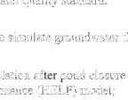
For

simplicity, HELP

percolation

rates

were

averaged

for

periods

where

there

was

little change

in

predicted

percolation

rate

(Figure 12).

River

Parameters

The Wabash

River and

tributaries

were

represented

by

head-dependent

flux

nodes

that

required

inputs

for

river

stage,

width,

bed

thickness,

and

bed

hydraulic

conductivity.

The

latter

three

parameters

were

used

to calculate

a

conductance term

for

the

boundary

node.

This

conductance term

was

determined

by

adjusting

hydraulic

conductivity during

model

calibration,

while

bed

thickness

was

set

at

1

(i.e.,

bed

hydraulic conductivity

represented

conductance normalized

for

river

width

and

bed

thickness).

River

stage

for

the

Wabash

River

was

set

near

mean

stage,

and

adjusted slightly during

calibration. River

stage

for

the tributaries

was

determined from

USGS

topographic

maps.

Sensitivity

analysis

showed

that

the

model

was

highly

sensitive to

the

presence

of

the

rivers

and

tributaries,

but

not

very

sensitive

to

the

conductance term

used.

Drain

Parameters

A

MODFLOW

drain

boundary

was

added

to

the

Pond

D

closure

model

to

evaluate

the

effect

of

a

groundwater

collection

trench

on

migration

south

of

Pond

D.

Drain

parameters

are

listed

in

Table

5.

MT3DMS

Input

Values and

Sensitivity

MT3DMS

input

values

are

listed

in

Table

3

and

described

below.

Initial

Concentration

Initial

groundwater

concentration for

the

calibration

run was

set

at

zero.

Initial

groundwater

concentration

for

the

Pond

D

closure simulations

was

the

final

calibration

concentration.

[TECH

M

EMO

-

MODEL.DOC]

9

NATURAL

RESOURCE

TECHNOLOGY

TSD

000502

---

TECHNICAL

MEMORANDUM

Source

Concentration

Two

primary

sources

were

simulated. For

calibration

runs,

which

simulated

in-service

conditions,

and

for

the

initial

portion

of

the

Pond

D

dewatering

simulation

(stress

periods

1

through 3)

the

primary

source

was

percolating

water

from Pond

D.

The

dominant

source

following

dewatering

of

Pond

D

is

leaching

of

ash

that

remains below

the

water

table.

Therefore,

a

second

primary

source

term,

representing

the

saturated

ash,

was

added

for

the

Pond

D

closure

simulation,

beginning

with model

stress

period

4

(after

one

year

of

dewatering). This

source

boundary

assumes

that

mass

loading

at

that

time

will

primarily

be

from

leaching

of

ash

below

the

water

table,

rather than

percolation.

Concentration values

for

the

ash cells

were

held

constant

during

calibration and

the

dewatering

period

of

the

Pond

D

closure

simulation,

and then

increased to

20 mg/L

after

the

cap

was

applied.

This change

assumes

that

constituent concentrations

in

leachate

will

increase

after

surface

water

accumulation

is

eliminated,

and

the

cap

is

applied,

due to

increased contact

time with

the

ash.

Secondary

sources

were

Pond

A

and

the

coal

pile.

Concentrations for

these

two

sources

were

set

at

20

and

2

mg/L,

respectively,

based

on

concentrations

in

leachate

samples

obtained

during

the

1999

hydrogeologic

assessment.

Concentrations

at

several

wells

were

sensitive to the

concentration

of

the

percolation

source

term.

Only

well

MW8

was

sensitive

to

the

concentration

of

the

saturated ash

source

term.

Effective Porosity

Effective

porosity

values

were

based

on

ranges

provided

by

Mercer

and

Waddel

(1993).

Predicted

concentrations

were

not

sensitive to

this

term,

so

it

was

not

adjusted during

calibration.

Dispersivity

One

well

(MW3)

was

highly

sensitive to

dispersivity

values,

and

the

value of

30

feet

was

selected

during

calibration

based

on

predicted

concentration at

that

well.

Transverse

and vertical

dispersion

were

estimated

according

to

ratios

developed

by

Gelhar et

al.

(1985).

Retardation

Retardation

was

calculated

by the

model

based

on

the

distribution

coefficient

(K<i).

The Kd

value

used

for

the

sandy

materials

in

this

model

(0.17

milliliters

per

gram,

or

mL/g)

was

based

on

testing performed

by

[TECHMEMO-MODEL.DOC]

10

NATURAL

RESOURCE

TECHNOLOGY

TSD

000503

---

TECHNICAL MEMORANDUM

NRT

for similar

materials

in

another

state.

The

K<i

value

for the

silt

materials

(0.85

mL/g)

was

assumed

a

factor

of

five

higher

than

that

for

sand.

These

Kd

values

were

slightly

lower

than

published

values

for

similar

materials

and

boron concentrations (0.44

L/kg

in

sand;

1.07

L/kg

in

silt

for

boron

at

5

mg/L;

EPRI,

2005).

While

concentrations

at

several

wells

varied

with

K<i,

no

concentrations

varied

by

more

than

10

percent,

so

this

number

was

not

adjusted during

calibration.

Input Data

Assumptions

Simplifying assumptions

were

made

while

developing

this

model,

including:

•

Leachate

is

assumed

to

instantaneously

reach

groundwater

(e.g.,

migrate through

the

unsaturated

zone);

•

River

stage

and natural

recharge

are

assumed constant

over

time;

and

•

Leachate concentrations

are

assumed

to

remain constant

over

time

(except

as

noted

Modeling Results

Results

of

the

MODFLOW/MT3DMS

modeling

are

presented

below.

A

disk containing

model

files

is

attached

to

the back

of

the

report.

Model

file

folder

names

are

listed

in

Table

7.

Calibration

The

model

was

calibrated

to

reproduce

conditions

while

Pond

D

was

active,

prior

to

2000.

The

model

was

first

calibrated to

observed

groundwater

head

data collected in

November

1998,

and then

to

observed

concentration

data

mostly

collected

from November

1998

through

May

1998.

An

exception

to

the

concentration

date

range

was

made

for

wells MW2

and

MW3.

Boron concentrations

at these

wells

were

affected

by

a

leaking

pipe that

was

not

simulated

in

the

model

because

the

volume

of

the

pipe

leak

was

unknown,

the

leak

was

temporary

(i.e.,

transient),

and

the

calibration

was

performed

for

steady-state

conditions.

Therefore,

these

wells

were

calibrated

to

the

concentration

range

recorded

prior

to

the

pipe

leak.

Head

calibration results

were

generally

good,

with

modeled heads

mostly

within

1

foot

of target

heads

(Figures

13a

and

14a),

particularly

between

and

downgradient

of

Ponds

A

and

D.

The

areas of

largest

discrepancy

were

near

MW6,

MW9,

and

MW11.

The

discrepancy

at

MW9

is

acceptable

given

its

distance

from

Ponds

A

and

D

and the

sparse

geologic

data in that

area.

The

discrepancies

at MW6 and

[TECH

MEMO

-

MODEL.DOC]

11

NATURAL

RESOURCE

TECHNOLOGY

TSD

000504

---

TECHNICAL

MEMORANDUM

MW11

are

likely

due

to

the

close

proximity

of

these

wells

to

Pond

D,

where

heads

change rapidly

over

a

short

distance.

Given

this

observation,

and

considering

that

the

concentration

match for

these

two

wells

was

acceptable,

the head

discrepancy

is

also

considered

acceptable.

Concentration

calibration

was

within

the

range

of

observed

concentrations

at

most

monitoring

wells

(Figure

13b

and

14b).

The

model calculated elevated

boron

concentrations

at

wells

with

observed boron

concentrations

greater

than Class

I

standards,

and

generally

did

not show

elevated

boron concentrations

for

wells

with

low

boron

concentrations.

The

two

notable

exceptions,

for

wells MW7D and

MW12,

were

both

cases where

the

model calculated

higher

concentrations

than

observed.

The

low

observed

concentration

at

MW7D could

not

be

replicated

without

using

unrealistically

low

hydraulic

conductivities,

and

would

have

probably required

several

additional

model

layers

to

simulate.

The

high

concentration

at MW12

is likely

due to

model

discretization. Concentration match

may

have

improved

with

a

finer

grid

spacing;

however,

this

result

was

conservatively

high,

and

such

a

grid

spacing

was

considered

unwarranted.

Slightly

low concentrations

were

predicted

for

MW6 and

MW13.

The

concentration

discrepancy

at

MW6

was

likely

due

to

model

discretization,

similar

to

MW12.

The

discrepancy

at

MW13, where

observed

boron concentration

was

higher

than

any

other

monitoring

well

on

site,

is likely

related

to

the

leak

that

was

not simulated.

Extent

of Southward

Migration

The

extent

of

migration

south

of

Pond

D

was

determined

based

on

the

results

of

the calibration

scenario,

when

southward

extent

was

greatest due

to

mounding

caused

by

the

large recharge

flux

modeled

from

the

pond.

This

distance

is

approximately

500

feet

south

of

the

south

property

line

(Figure

15),

and

represents

a

conservative

approach

to

calculating

this

value

since

the

impoundment

has

not

been

ponded

since

2000.

This

estimate

is

also

conservative

because

the

model-predicted southward

extent

of

boron,

as

defined

by

concentrations

higher

than

Class

I

standards,

will

be

greater

than

for

the

other

ash

indicator

constituent,

sulfate.

This

is

because

the

source

boron

concentration

of

20

mg/L

is

an

order

of

magnitude higher

than

its

Class

I

standard,

while

the

highest

sulfate

concentrations observed

in

leachate

samples

from

the ash

ponds (1,326 mg/L)

and

in

Pond

D

monitoring

wells

(960

mg/L)

are

only a

factor

of

three to

four

higher

than

its

Class

I

standard.

Pond

D

Closure

Simulation

Two

scenarios

were

performed

for

Pond

D

closure, one

with

a

groundwater

collection

trench

and

one

without

a

groundwater

collection

trench.

Without

the

trench,

boron concentrations

south

of

the

property

[TECHMEMO-MODEL.DOC]

12

NATURAL

RESOURCE

TECHNOLOGY

TSD

000505

---

TECHNICAL

MEMORANDUM

boundary

were

predicted

to

be

below

Class

I

standards after

17

years.

With the

trench,

boron

concentrations

were

predicted

to be

below

Class

I

standards

after

10

years

(Figure 16).

The

site-wide

decrease

in

plume extent

over

time

is

shown

in

Figure

17.

The

model-predicted

rate

ofgroundwater

collection

in

the

trench

was

62

gpm

(Table

6).

Boron

Loading

to

the

Wabash

River

The model

was

used

to

calculate

boron

loading

rate

in

groundwater discharge

to

the

Wabash

River

and

tributaries.

The

results

of

this

analysis

indicated

an

84

percent

decrease

in

loading

rate

after

3

years

of

dewatering,

and

97

percent

decrease

relative

the calibrated

rate

of boron

loading

one

year

after

the

cap

was

simulated

(Figure

References

EPRI,

2005,

Chemical

Constituents

in

Coal Combustion Product

Leachate:

Boron,

Electric

Power

Research

Institute

Technical

Report

1005258.

Gelhar,

L.W.,

A.

Mantoglou,

C.

Welty,

and

K.R.

Rehfeldt, 1985,

.4

Review

of

Field-Scale

Physical

Solute

Transport Processes

in