| | - Regional Air Quality Analyses for Ozone, PM2.5, and Regional Haze:
- Final Technical Support Document
- Table of Contents
- Section-Title Page
- Appendix I Ozone and PM2.5 Modeling Results
- Appendix IV Haze Source Apportionment Modeling Results
- EXECUTIVE SUMMARY
- Figure i. Current nonattainment counties for ozone (left) and PM2.5 (right)
- Section 1.0 Introduction
- 1.1 SIP Requirements
- 1.2 Organization
- Section 2.0 Ambient Data Analyses
- 2.1 Ozone
- Figure 1. 8-hour ozone design values (2005-2007)
- Figure 2. Number of hot days and 8-hour “exceedance” days in 5-state region
- Figure 4. Examples of recent high ozone days in the Lake Michigan area
- Figure 8 Ozone design value trends in 5-State region
- Figure 9. Trend in ozone design values and 4
- th high values for higher ozone sites in region
- Figure 10. Ozone design value maps for 1995-1997, 2000-2002, and 2005-2007
- Figure 11a. Trends in meteorologically adjusted 4
- th high 8-hour ozone
- concentrations for seven Midwestern sites (1997 – 2007)
- Note: line represents linear best fit
- Extent Range Precursor Sensitivity
- Figure 14. Mean afternoon extent of reaction (1998 – 2002)
- Table 2. PM2.5 Data for Select Sites in 5-State Region
- Figure 17. Percent of days in AQI categories for PM2.5 (2002-2004)
- Figure 20. Annual trends in PM2.5 mass (1999 – 2006)
- Figure 21. Seasonal trends in PM2.5 mass (1999 – 2006)
- Figure 22 Day-of-week variability in PM2.5 (2002-2004)
- Figure 23. Spatial map of PM2.5 chemical composition in the Midwest (2002-2003)
- Figure 25 Seasonal and spatial variability in PM2.5 components
- Table 3. Average of 20% worst days, with and without missing data days
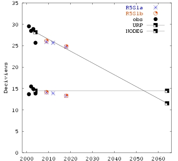
- Table 4. Summary of visibility metrics (deciviews) for northern Class I areas
- 20% Best Days 20% Worst Days
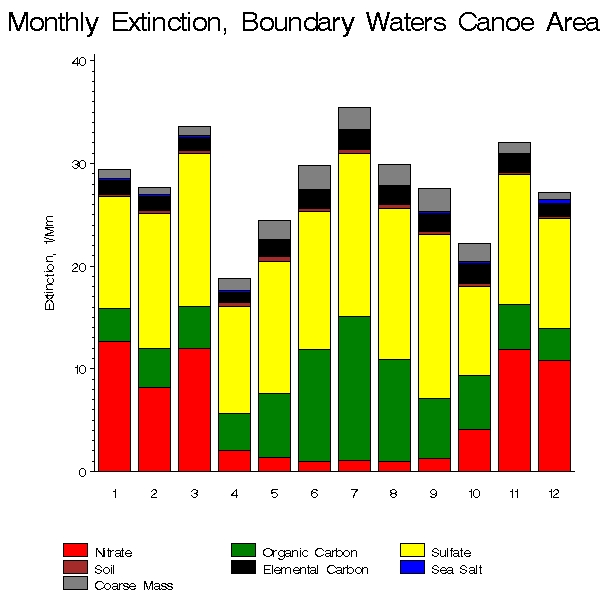
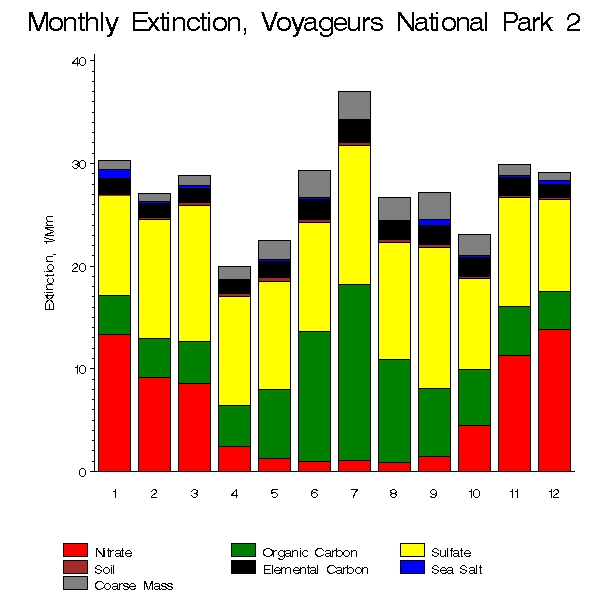
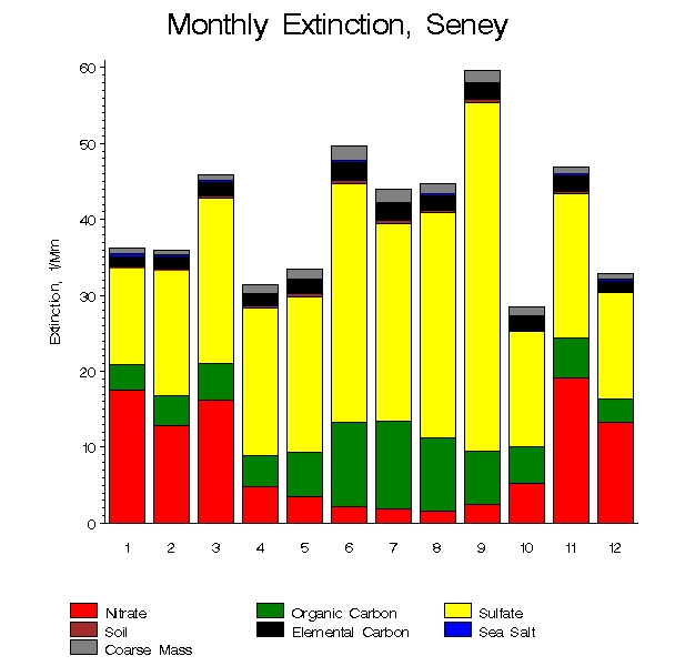
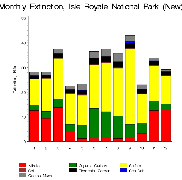
- Figure 33. Monthly average light extinction values for northern Class I areas
- in sulfate, nitric acid, and ammonia
- organic carbon species in Seney (bottom)
- Table 5. Days with high OC and EC concentrations in northern Class I areas
- Section 3.0 Air Quality Modeling
- 3.1 Selection of Base Year
- 3.2 Future Years of Interest
- 3.3 Modeling System
- Base M (2005) Base K (2002)
- 3.4 Domain/Grid Resolution
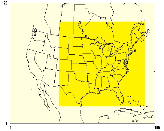
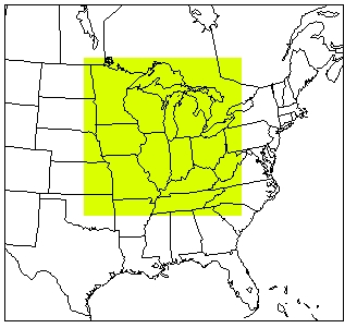
- Figure 37. Modeling grids – RPO domain (left) and LADCO modeling domain (right)
- 12 km
- 36 km
- Figure 38. MM5 modeling domain for 2001-2003 (left) and 2005 (right)
- VOC NOx SO2
- VOC Emissions NOx Emissions
- Figure 44. Isoprene emissions for Base M (left) v. Base K (right)
- Figure 46. Ammonia emissions for a July weekday (2005) – 12 km modeling domain
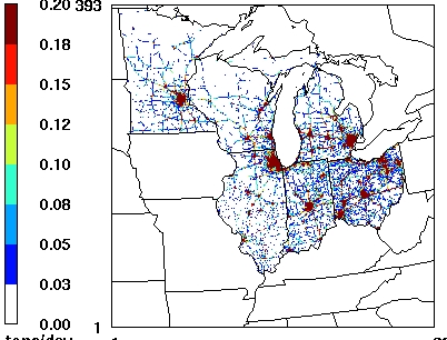
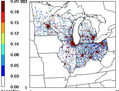
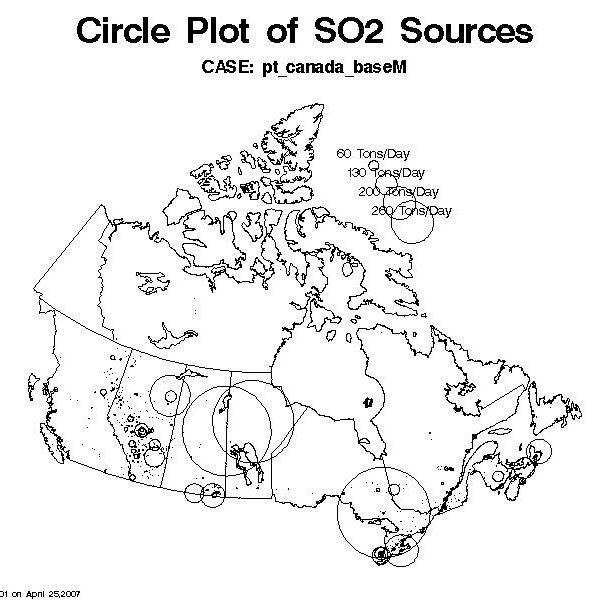
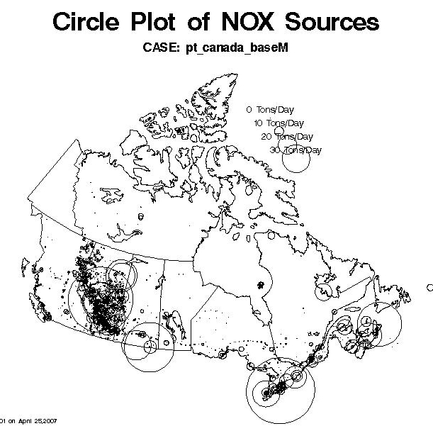
- Figure 47. Canadian point source emissions for SO2 (left) and NOx (right)
- VOC NOx SO2
- Figure 50. Mean bias for summer 2005 (Base M) and summer 2002 (Base K)
- Figure 51. Mean bias (left) and gross error (right) for summer 2005
- Figure 52. 4 km grids for Lake Michigan region and Detroit-Cleveland region
- Base M (left column) and Base K (right column)
- SULFATE NITRATE ORGANIC CARBON
- SULFATE NITRATE ORGANIC CARBON
- 2005 (observed) 2009
- 2012 2018
- 2005 (observed) 2009
- 2012 2018
- 2005 (observed) 2009
- 2012 2018
- Table 11. Number of sites above standard
- Ozone (8 hour: 85 ppb)
- PM2.5 (Annual: 15 ug/m3)
- Area Name Category
- Number of
- Counties
- Attainment Deadline
- Figure 64. Estimated Future Year Values (unmonitored grid cells)
- Holland
- Section 5. Reasonable Progress Assessment for Regional Haze
- 5.1 Class I Areas Impacted
- Table 14. Draft List of Class I Areas Impacted by LADCO States
- AREA NAME IL IN MI OH WI
- 81.401 Alabama.
- 81.408 Georgia.
- 81.411 Kentucky.
- 81.412 Louisiana.
- 81.413 Maine.
- 81.414 Michigan.
- 81.415 Minnesota.
- 81.416 Missouri.
- 81.419 New Hampshire.
- 81.42 New Jersey.
- 81.428 Tennessee.
- 81.431 Vermont.
- 81.433 Virginia.
- 81.435 West Virginia.
- Voyageurs Boundary Waters
- Isle Royale Seney
- Mammoth Cave Upper Buffalo
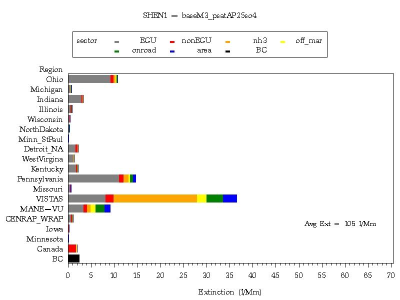
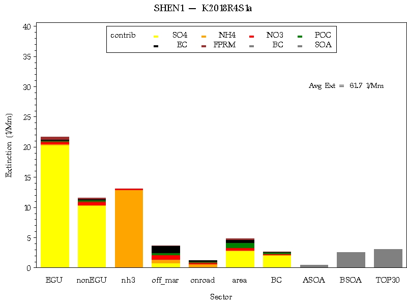
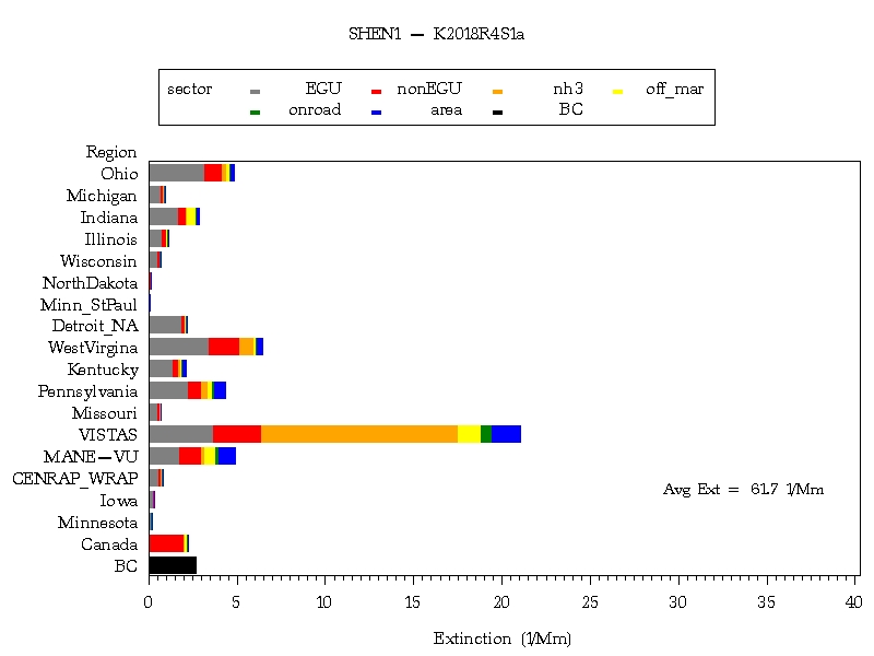
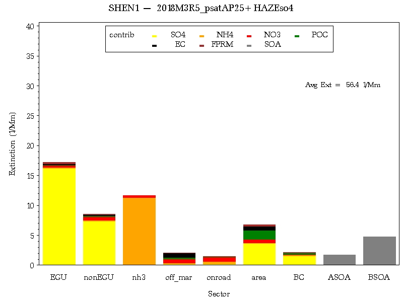
- Figure 73. Visibility modeling results for Class I areas in eastern U.S.
- Mingo Shenandoah
- Dolly Sods Bringantine
- Lye Brook Acadia
- Table 15. Haze Results - Round 4 (Based on 2000-2004)
- Table 16. Haze Results - Round 5.1 (Based on 2000-2004)
- Table 17. Estimated Cost Effectiveness for Potential Control Measures
- Visibility Improvement (dv)
- EGUs ICI Boilers Rec.Eng. Mobile Ag
- EGUs ICI Boilers Rec.Eng. Mobile Ag
- Table 18. Haze Results - Round 5.1 (Based on 2000-2005)
- Seney Isle Royale
- Boundary Waters Voyageurs
- Table 19. State Culpabilities Based on PSAT Modeling and Trajectory Analyses
- Boundary Waters Seney
- Voyageurs Isle Royale
- Section 6. Summary
- Section 7. References
- APPENDIX I
- PM2.5 RRFs by Species and Season (2009)
- APPENDIX II
- Ozone Source Apportionment Modeling Results
- APPENDIX III
- PM2.5 Source Apportionment Modeling Results
- Chicago (Cicero), Illinois
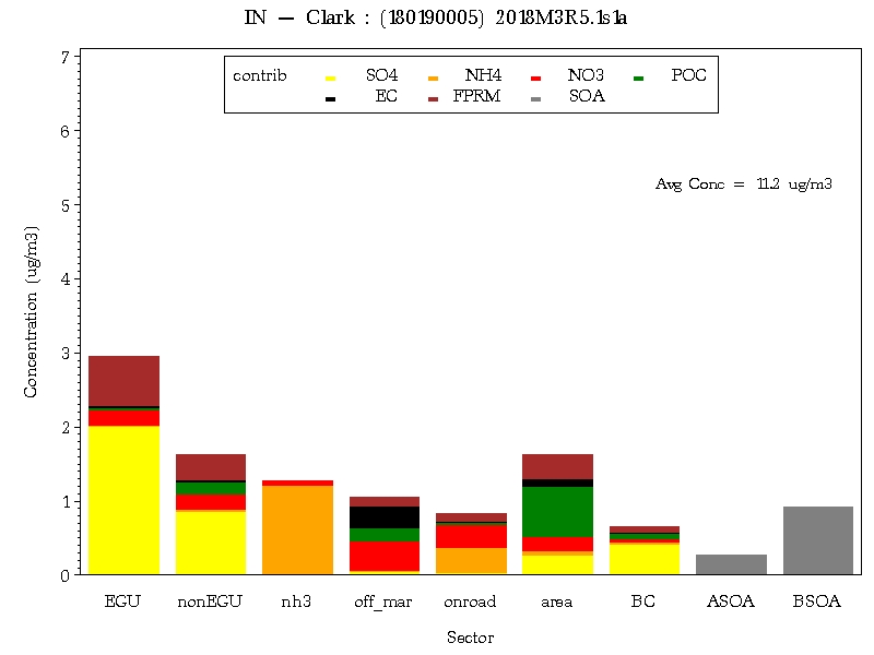
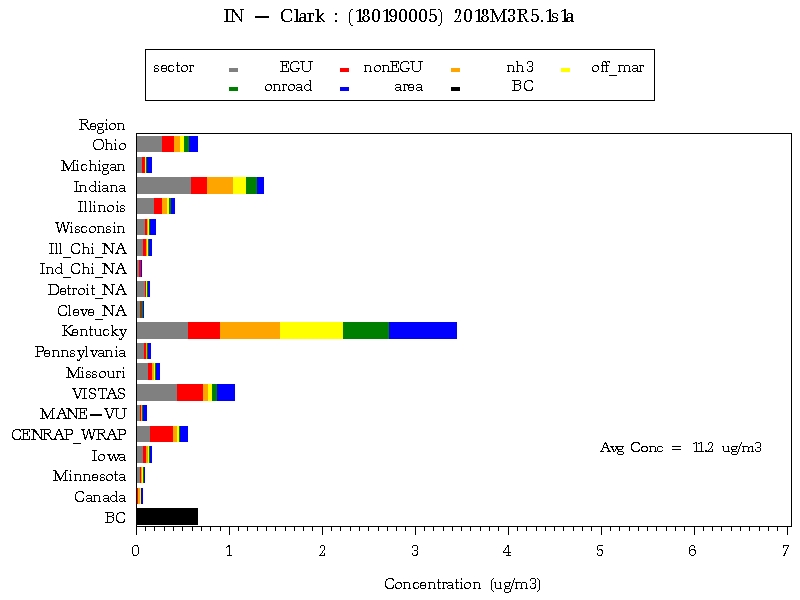
- Clark County, Indiana
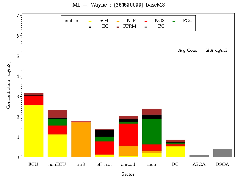
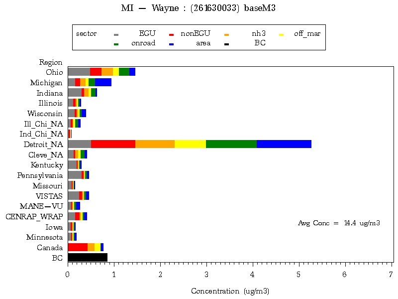
- Dearborn, Michigan
- Cincinnati, Ohio
- Cleveland, Ohio
- Steubenville, Ohio
- APPENDIX IV
- Boundary Waters, Minnesota
- Voyageurs, Minnesota
- Seney, Michigan
- Isle Royale, Michigan
- Shenandoah, Virginia
- Mammoth Cave, Kentucky
- Lye Brook, Vermont
|


Regional Air Quality Analyses for
Ozone, PM
2.5
, and Regional Haze:
Final Technical Support Document
April 25, 2008
States of Illinois, Indiana, Michigan, Ohio, and Wisconsin
Electronic Filing - Received, Clerk's Office, January 21, 2009
Appendix A
ii
Table of Contents
Section-Title
Page
Executive Summary
iii
1.0
Introduction
1
1.1
SIP Requirements
1
1.2
Organization
2
1.3
Technical Work: Overview
3
2.0
Ambient Data Analyses
4
2.1
Ozone
4
2.2
PM
2.5
21
2.3
Regional Haze
35
3.0
Air Quality Modeling
46
3.1
Selection of Base Year
46
3.2
Future Years of Interest
46
3.3
Modeling System
47
3.4
Domain/Grid Resolution
47
3.5
Model Inputs: Meteorology
48
3.6
Model Inputs: Emissions
51
3.7
Base Year Modeling Results
60
4.0
Attainment Demonstration for Ozone and PM
2.5
71
4.1
Future Year Modeling Results
71
4.2
Supplemental Analyses
82
4.3
Weight of Evidence Determination for Ozone
82
4.4
Weight of Evidence Determination for PM
2.5
90
5.0
Reasonable Progress Assessment for Regional Haze
93
5.1
Class I Areas Impacted
93
5.2
Future Year Modeling Results
96
5.3
Weight of Evidence Determination for Regional Haze
104
6.0
Summary
111
7.0
References
114
Appendix I Ozone and PM
2.5
Modeling Results
Appendix II Ozone Source Apportionment Modeling Results
Appendix III PM
2.5
Source Apportionment Modeling Results
Appendix IV Haze Source Apportionment Modeling Results
iii
EXECUTIVE SUMMARY
States in the upper Midwest face a number of air quality challenges. More than 50 counties are
currently classified as nonattainment for the 8-hour ozone standard and 60 for the fine particle
(PM
2.5
) standard (1997 versions). A map of these nonattainment areas is provided in the figure
below. In addition, visibility impairment due to regional haze is a problem in the larger national
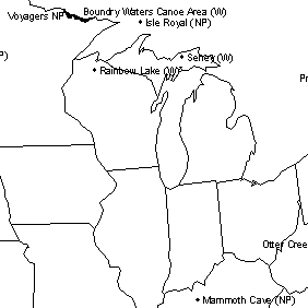
parks and wilderness areas (i.e., Class I areas). There are 156 Class I areas in the U.S.,
including two in northern Michigan.
Figure i. Current nonattainment counties for ozone (left) and PM
2.5
(right)
To support the development of State Implementation Plans (SIPs) for ozone, PM
2.5
, and
regional haze in the States of Illinois, Indiana, Michigan, Ohio, and Wisconsin, technical
analyses were conducted by the Lake Michigan Air Directors Consortium (LADCO), its member
states, and various contractors. The analyses include preparation of regional emissions
inventories and meteorological data, evaluation and application of regional chemical transport
models, and collection and analysis of ambient monitoring data.
Monitoring data were analyzed to produce a conceptual understanding of the air quality
problems. Key findings of the analyses include:
Ozone
•
Current monitoring data (2005-2007) show about 20 sites in violation of the 8-hour
ozone standard of 85 parts per billion (ppb). Historical ozone data show a steady
downward trend over the past 15 years, especially since 2001-2003, due likely to
federal and state emission control programs.
•
Ozone concentrations are strongly influenced by meteorological conditions, with
more high ozone days and higher ozone levels during summers with above normal
temperatures.
iv
•
Inter- and intra-regional transport of ozone and ozone precursors affects many
portions of the five states, and is the principal cause of nonattainment in some areas
far from population or industrial centers.
PM
2.5
•
Current monitoring data (2005-2007) show 30 sites in violation of the annual PM
2.5
standard of 15 ug/m
3
. Nonattainment sites are characterized by an elevated
regional background (about 12 – 14 ug/m
3
) and a significant local (urban) increment
(about 2 – 3 ug/m
3
). Historical PM
2.5
data show a slight downward trend since
deployment of the PM
2.5
monitoring network in 1999.
•
PM
2.5
concentrations are also influenced by meteorology, but the relationship is
more complex and less well understood compared to ozone.
•
On an annual average basis, PM
2.5
chemical composition consists mostly of sulfate,
nitrate, and organic carbon in similar proportions.
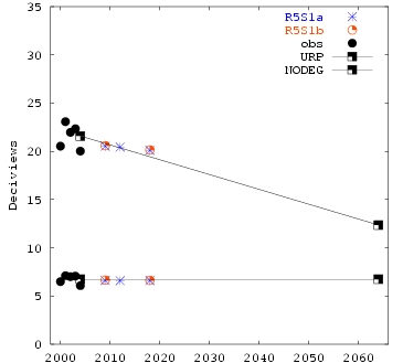
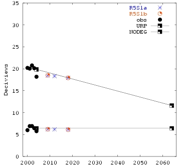
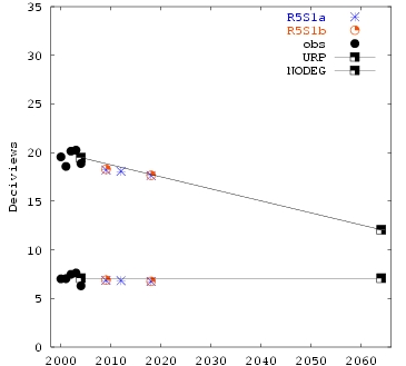
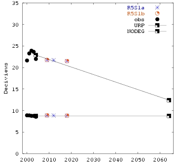
Haze
•
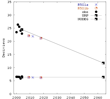
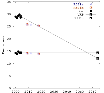
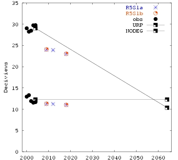
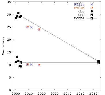
Current monitoring data (2000-2004) show visibility levels in the Class I areas in
northern Michigan are on the order of 22 – 24 deciviews. The goal of EPA’s visibility
program is to achieve natural conditions, which is about 12 deciviews for these
Class I areas, by the year 2064.
•
Visibility impairment is dominated by sulfate and nitrate.
Air quality models were applied to support the regional planning efforts. Two base years were
used in the modeling analyses: 2002 and 2005. Basecase modeling was conducted to evaluate
model performance (i.e., assess the model's ability to reproduce observed concentrations). This
exercise was intended to build confidence in the model prior to its use in examining control
strategies. Model performance for ozone and PM
2.5
was found to be generally acceptable.
Future year strategy modeling was conducted to determine whether existing (“on the books”)
controls would be sufficient to provide for attainment of the standards for ozone and PM
2.5
and if
not, then what additional emission reductions would be necessary for attainment. Based on the
modeling and other supplemental analyses, the following general conclusions can be made:
•
Existing controls are expected to produce significant improvement in ozone and
PM
2.5
concentrations and visibility levels.
•
The choice of the base year affects the future year model projections. A key
difference between the base years of 2002 and 2005 is meteorology. 2002 was
more ozone conducive than 2005. The choice of which base year to use as the
basis for the SIP is a policy decision (i.e., how much safeguard to incorporate).
•
Modeling suggests that most sites are expected to meet the current 8-hour ozone
standard by the applicable attainment date, except for sites in western Michigan
and, possibly, in eastern Wisconsin and northeastern Ohio.
v
•
Modeling suggests that most sites are expected to meet the current PM
2.5
standard by the applicable attainment date, except for sites in Detroit, Cleveland,
and Granite City.
The regional modeling for PM
2.5
does not include air quality benefits expected
from local controls. States are conducting local-scale analyses and will use
these results, in conjunction with the regional-scale modeling, to support their
attainment demonstrations for PM
2.5
.
•
These findings of residual nonattainment for ozone and PM
2.5
are supported by
current (2005 – 2007) monitoring data which show significant nonattainment in
the region (e.g., peak ozone design values on the order of 90 – 93 ppb, and peak
PM
2.5
design values on the order of 16 - 17 ug/m
3
). It is unlikely that sufficient
emission reductions will occur in the next couple of years to provide for
attainment at all sites.
•
Attainment at most sites by the applicable attainment date is dependent on actual
future year meteorology (e.g., if the weather conditions are consistent with [or
less severe than] 2005, then attainment is likely) and actual future year
emissions (e.g., if the emission reductions associated with the existing controls
are achieved, then attainment is likely). If either of these conditions is not met,
then attainment may be less likely.
•
Modeling suggests that the new PM
2.5
24-hour standard and the new lower
ozone standard will not be met at several sites, even by 2018, with existing
controls.
•
Visibility levels in a few Class I areas in the eastern U.S. are expected to be
greater than (less improved than) the uniform rate of visibility improvement
values in 2018 based on existing controls, including those in northern Michigan
and some in the northeastern U.S. Visibility levels in many other Class I areas in
the eastern U.S. are expected to be less than (more improved than) the uniform
rate of visibility improvement values in 2018. These results, along with
information on the costs of compliance, time necessary for compliance, energy
and non air quality environmental impacts of compliance, and remaining useful
life of existing sources, should be considered by the states in setting reasonable
progress goals for regional haze.
1
Section 1.0 Introduction
This Technical Support Document summarizes the final air quality analyses conducted by the
Lake Michigan Directors Consortium (LADCO)
1
and its contractors to support the development
of State Implementation Plans (SIPs) for ozone, fine particles (PM
2.5
), and regional haze in the
States of Illinois, Indiana, Michigan, Ohio, and Wisconsin. The analyses include preparation of
regional emissions inventories and meteorological modeling data for two base years (2002 and
2005), evaluation and application of regional chemical transport models, and analysis of
ambient monitoring data.
Two aspects of the analyses should be emphasized. First, a regional, multi-pollutant approach
was taken in addressing ozone, PM
2.5
, and haze for technical reasons (e.g., commonality in
precursors, emission sources, atmospheric processes, transport influences, and geographic
areas of concern), and practical reasons (e.g., more efficient use of program resources).
Furthermore, EPA has consistently encouraged multi-pollutant planning in its rule for the haze
program (64 FR 35719), and its implementation guidance for ozone (70 FR 71663) and PM
2.5
(72 FR 20609). Second, a weight-of-evidence approach was taken in considering the results of
the various analyses (i.e., two sets of modeling results -- one for a 2002 base year and one for a
2005 base year -- and ambient data analyses) in order to provide a more robust assessment of
expected future year air quality.
The report is organized in the following sections. This Introduction provides an overview of
regulatory requirements and background information on regional planning. Section 2 reviews
the ambient monitoring data and presents a conceptual model of ozone, PM
2.5
, and haze for the
region. Section 3 discusses the air quality modeling analyses, including development of the key
model inputs (emissions inventory and meteorological data), and basecase model performance
evaluation. A modeled attainment demonstration for ozone and PM
2.5
is presented in Section 4,
along with relevant data analyses considered as part of the weight-of-evidence determination.
Section 5 documents the reasonable progress assessment for regional haze, along with
relevant data analyses considered as part of the weight-of-evidence determination. Finally, key
study findings are reviewed and summarized in Section 6.
1.1 SIP Requirements
For ozone, EPA promulgated designations on April 15, 2004 (69 FR 23858, April 30, 2004). In
the 5-state region, more than 100 counties were designated as nonattainment.
2
The
designations became effective on June 15, 2004. SIPs for ozone were due no later than three
years from the effective date of the nonattainment designations (i.e., by June 2007). The
attainment date for ozone varies as a function of nonattainment classification. For the region,
the attainment dates are either June 2007 (marginal nonattainment areas), June 2009 (basic
nonattainment areas), or June 2010 (moderate nonattainment areas).
1
A sub-entity of LADCO, known as the Midwest Regional Planning Organization (MRPO), is responsible
for the regional haze activities of the multi-state organization.
2
Based on more recent air quality data, many counties in Indiana, Michigan, and Ohio were
subsequently redesignated as attainment. As of December 31, 2007, there are 53 counties designated
as nonattainment in the region.
Electronic Filing - Received, Clerk's Office, January 21, 2009
Appendix A
2
For PM
2.5
, EPA promulgated designations on December 17, 2004 (70 FR 944, January 5, 2005).
In the 5-state region, 70 counties were designated as nonattainment.
3
The designations became
effective on April 5, 2005. SIPs for PM
2.5
are due no later than three years from the effective
date of the nonattainment designations (per section 172(b) of the Clean Air Act) (i.e., by April
2008) and for haze no later than three years after the date on which the Administrator
promulgated the PM
2.5
designations (per the Omnibus Appropriations Act of 2004) (i.e., by
December 2007). The applicable attainment date for PM
2.5
nonattainment areas is five years
from the date of the nonattainment designation (i.e., by April 2010).
For haze, the Clean Air Act sets “as a national goal the prevention of any future, and the
remedying of any existing, impairment of visibility in Class I areas which impairment results from
manmade air pollution.” There are 156 Class I areas, including two in northern Michigan: Isle
Royale National Park and Seney National Wildlife Refuge
4
. EPA’s visibility rule (64 FR 35714,
July 1, 1999) requires reasonable progress in achieving “natural conditions” by the year 2064.
As noted above, the first regional haze SIP was due in December 2007 and must address the
initial 10-year implementation period (i.e., reasonable progress by the year 2018). SIP
requirements (pursuant to 40 CFR 51.308(d)) include setting reasonable progress goals,
determining baseline conditions, determining natural conditions, providing a long-term control
strategy, providing a monitoring strategy (air quality and emissions), and establishing BART
emissions limitations and associated compliance schedule.
1.2 Organization
LADCO was established by the States of Illinois, Indiana, Michigan, and Wisconsin in 1989. The
four states and EPA signed a Memorandum of Agreement (MOA) that initiated the Lake
Michigan Ozone Study (LMOS) and identified LADCO as the organization to oversee the study.
Additional MOAs were signed by the States in 1991 (to establish the Lake Michigan Ozone
Control Program), January 2000 (to broaden LADCO’s responsibilities), and June 2004 (to
update LADCO’s mission and reaffirm the commitment to regional planning). In March 2004,
Ohio joined LADCO. LADCO consists of a Board of Directors (i.e., the State Air Directors), a
technical staff, and various workgroups. The main purposes of LADCO are to provide technical
assessments for and assistance to its member states, and to provide a forum for its member
states to discuss regional air quality issues.
MRPO is a similar entity led by the five LADCO States and involves the federally recognized
tribes in Michigan and Wisconsin, EPA, and Federal Land Managers (i.e., National Park
Service, U.S. Fish & Wildlife Agency, and U.S. Forest Service). In October 2000, the States of
Illinois, Indiana, Michigan, Ohio, and Wisconsin signed an MOA that established the MRPO. An
operating principles document for MRPO, which describe the roles and responsibilities of states,
tribes, federal agencies, and stakeholders, was issued in March 2001. MRPO has a similar
purpose as LADCO, but is focused on visibility impairment due to regional haze in the Federal
Class I areas located inside the borders of the five states, and the impact of emissions from the
five states on visibility impairment due to regional haze in the Federal Class I areas located
outside the borders of the five states. MRPO works cooperatively with the Regional Planning
Organizations (RPOs) representing other parts of the country. The RPOs sponsored several
3
USEPA subsequently adjusted the final designations, which resulted in 63 counties in the region being
designated as nonattainment (70 FR 19844, April 15, 2005).
4
Although Rainbow Lake in northern Wisconsin is also a Class I area, the visibility rule does not apply
because the Federal Land Manager determined that visibility is not an air quality related value there.
3
joint projects and, with assistance by EPA, maintain regular contact on technical and policy
matters.
1.3 Technical Work: Overview
To ensure the reliability and effectiveness of its planning process, LADCO has made data
collection and analysis a priority. More than $7M in RPO grant funds were used for special
purpose monitoring, preparing and improving emissions inventories, and conducting air quality
analyses
5
. An overview of the technical work is provided below.
Monitoring: Numerous monitoring projects were conducted to supplement on-going state and
local air pollution monitoring. These projects include rural monitoring (e.g., comprehensive
sampling in the Seney National Wildlife Refuge and in Bondville, IL); urban monitoring (e.g.,
continuation of the St. Louis Supersite); aloft (aircraft) measurements; regional ammonia
monitoring; and organic speciation sampling in Seney, Bondville, and five urban areas.
Emissions: Baseyear emissions inventories were prepared for 2002 and 2005. States provided
point source and area source emissions data, and MOBILE6 input files and mobile source
activity data. LADCO and its contractors developed the emissions data for other source
categories (e.g., select nonroad sources, ammonia, fires, and biogenics) and processed the
data for input into an air quality model. To support control strategy modeling, future year
inventories were prepared. The future years of interest include 2008 (planning year to address
the 2009 attainment year for basic ozone nonattainment ares), 2009 (planning year to address
the 2010 attainment year for PM
2.5
and moderate ozone nonattainment areas), 2012 (planning
to address a 2013 alternative attainment date), and 2018 (first milestone year for regional haze).
Air Quality Analyses: The weight-of-evidence approach relies on data analysis and modeling.
Air quality data analyses were used to provide both a conceptual model (i.e., a qualitative
description of the ozone, PM
2.5
, and regional haze problems) and supplemental information for
the attainment demonstration. Given uncertainties in emissions inventories and modeling,
especially for PM
2.5
, these data analyses are a necessary part of the overall technical support.
Modeling includes baseyear analyses for 2002 and 2005 to evaluate model performance and
future year strategy analyses to assess candidate control strategies. The analyses were
conducted in accordance with EPA’s modeling guidelines (EPA, 2007a). The PM/haze
modeling covers the full calendar year (2002 and 2005) for an eastern U.S. 36 km domain, while
the ozone modeling focuses on the summer period (2002 and 2005) for a Midwest 12 km
subdomain. The same model (CAMx) was used for ozone, PM
2.5
, and regional haze.
5
Since 1999, MRPO has received almost $10M in RPO grant funds from USEPA.
Electronic Filing - Received, Clerk's Office, January 21, 2009
Appendix A
4
Section 2.0 Ambient Data Analyses
An extensive network of air quality monitors in the 5-state region provides data for ozone (and
its precursors), PM
2.5
(both total mass and individual chemical species), and visibility. These
data are used to determine attainment/nonattainment designations, support SIP development,
and provide air quality information to public (see, for example, www.airnow.gov
).
Analyses of the data were conducted to produce a conceptual model, which is a qualitative
summary of the physical, chemical, and meteorological processes that control the formation and
distribution of pollutants in a given region. This section reviews the relevant data analyses and
describes our understanding of ozone, PM
2.5,
and regional haze with respect to current
conditions, data variability (spatial, temporal, and chemical), influence of meteorology (including
transport patterns), precursor sensitivity, and source culpability.
2.1 Ozone
In 1979, EPA adopted an ozone standard of 0.12 ppm, averaged over a 1-hour period. This
standard is attained when the number of days per calendar year with maximum hourly average
concentrations above 0.12 ppm is equal to or less than 1.0, averaged over a 3-year period,
which generally reflects a design value (i.e., the 4
th
highest daily 1-hour value over a 3-year
period) less than 0.12 ppm.
In 1997, EPA tightened the ozone standard to 0.08 ppm, averaged over an 8-hour period
6
. The
standard is attained if the 3-year average of the 4th-highest daily maximum 8-hour average
ozone concentrations (i.e., the design value) measured at each monitor within an area is less
than 0.08 ppm (or 85 ppb).
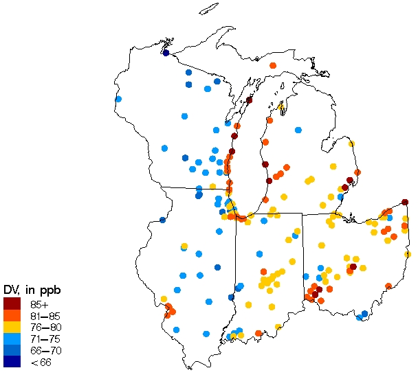
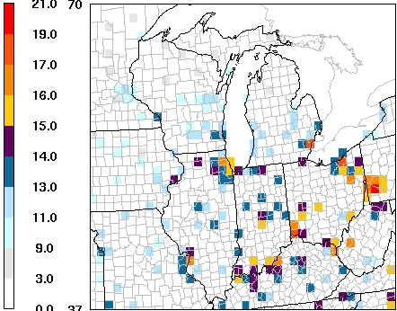
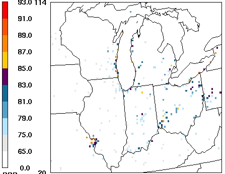
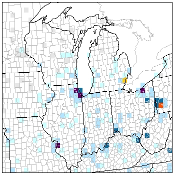
Current Conditions:
A map of the 8-hour ozone design values at each monitoring site in the
region for the 3-year period 2005-2007 is shown in Figure 1. The “hotter” colors represent
higher concentrations, where yellow and orange dots represent sites with design values above
the standard. Currently, there are 19 sites in violation of the 8-hour ozone NAAQS in the 5-state
region, including sites in the Lake Michigan area, Detroit, Cleveland, Cincinnati, and Columbus.
Table 1 provides the 4
th
-highest daily 8-hour ozone values and the associated design values
since 2001 for several high monitoring sites throughout the region.
6
On March 12, 2008, USEPA further tightened the 8-hour ozone standard to increase public health
protection and prevent environmental damage from ground-level ozone. USEPA set the primary (health)
standard and secondary (welfare) standard at the same level: 0.075 ppm (75 ppb), averaged over an 8-
hour period.
Electronic Filing - Received, Clerk's Office, January 21, 2009
Appendix A
5
Figure 1. 8-hour ozone design values (2005-2007)
Electronic Filing - Received, Clerk's Office, January 21, 2009
Appendix A
Key Sites
'01
'02
'03
'04
'05
'06
'07
'01-'03
'02-'04 '03-'05 '04-'06 '05-'07
Lake Michigan Area
Chiwaukee
99 116
88
78
93
79
85
101
94
86
83
85
Racine
92 111
82
69
95
71
77
95
87
82
78
81
Milwaukee-Bayside
93
99
92
73
93
73
83
94
88
86
79
83
Harrington Beach
102
93
99
72
94
72
84
98
88
88
79
83
Manitowoc
97
83
92
74
95
78
85
90
83
87
82
86
Sheboygan
102 105
93
78
97
83
88
100
92
89
86
89
Kewaunee
90
92
97
73
88
76
85
93
87
86
79
83
Door County
95
95
93
78 101
79
92
94
88
90
86
90
Hammond
90 101
81
67
87
75
77
90
83
78
76
79
Whiting
64
88
81
88
77
85
Michigan City
90 107
82
70
84
75
73
93
86
78
76
77
Ogden Dunes
85 101
77
69
90
70
84
87
82
78
76
81
Holland
92 105
96
79
94
91
94
97
93
89
88
93
Jenison
86
93
91
69
86
83
88
90
84
82
79
85
Muskegon
95
96
94
70
90
90
86
95
86
84
83
88
Indianapolis Area
Noblesville
88 101 101
75
87
77
84
96
92
87
79
82
Fortville
89 101
92
72
80
75
81
94
88
81
75
78
Fort B. Harrison
87 100
91
73
80
76
83
92
88
81
76
79
Detroit Area
New Haven
95
95 102
81
88
78
93
97
92
90
82
86
Warren
94
92 101
71
89
78
91
95
88
87
79
86
Port Huron
84 100
87
74
88
78
89
90
87
83
80
85
Cleveland Area
Ashtabula (Conneaut)
97 103
99
81
93
86
92
99
94
91
86
90
Notre Dame (Geauga)
99 115
97
75
88
70
68
103
95
86
77
75
Eastlake (Lake)
89 104
92
79
97
83
74
95
91
89
86
84
Akron (Summit)
98 103
89
77
89
77
91
96
89
85
81
85
Cincinnati Area
Wilmington (Clinton)
93
99
96
78
83
81
82
96
91
85
80
82
Sycamore (Hamilton)
88 100
93
76
89
81
90
93
89
86
82
86
Hamilton (Butler)
83 100
94
75
86
79
91
92
89
85
80
85
Middleton (Butler)
87
98
83
76
88
76
91
89
85
82
80
85
Lebanon (Warren)
85
98
95
81
92
86
88
92
91
89
86
88
Columbus Area
London (Madison)
84
97
90
75
81
76
83
90
87
82
77
80
New Albany (Franklin)
90 103
94
78
92
82
87
95
91
88
84
87
Franklin (Franklin)
83
99
84
73
86
79
79
88
85
81
79
81
Ohio Other Areas
Marietta (Washington)
85
95
80
77
88
81
86
86
84
81
82
85
St. Louis Area
W. Alton (MO)
85
99
91
77
89
91
89
91
89
85
85
89
Orchard (MO)
88
98
90
76
92
92
83
92
88
86
86
89
Sunset Hills (MO)
88
98
88
70
89
80
89
91
85
82
79
86
Arnold (MO)
86
93
82
70
92
79
87
87
81
81
80
86
Margaretta (MO)
80
98
90
72
91
76
91
89
86
84
79
86
Maryland Heights (MO)
88
84
94
88
4th High 8-hour Value
Design Values
Table 1. Ozone Data for Select Sites in 5-State Region
Electronic Filing - Received, Clerk's Office, January 21, 2009
Appendix A
7
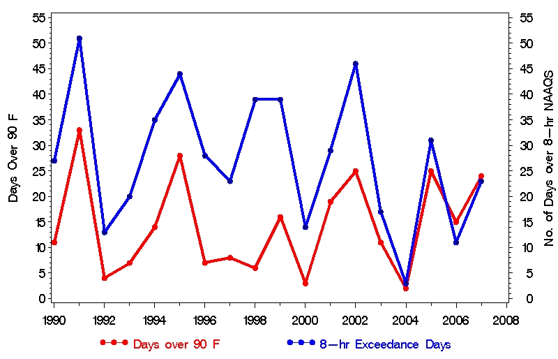
Meteorology and Transport:
Most pollutants exhibit some dependence on meteorological
factors, especially wind direction, because that governs which sources are upwind and thus
most influential on a given sample. Ozone is even more dependent, since its production is
driven by high temperatures and sunlight, as well as precursor concentrations (see, for
example, Figure 2).
Figure 2. Number of hot days and 8-hour “exceedance” days in 5-state region
Qualitatively, ozone episodes in the region are associated with hot weather, clear skies
(sometimes hazy), low wind speeds, high solar radiation, and southerly to southwesterly winds.
These conditions are often a result of a slow-moving high pressure system to the east of the
region. The relative importance of various meteorological factors is discussed later in this
section.
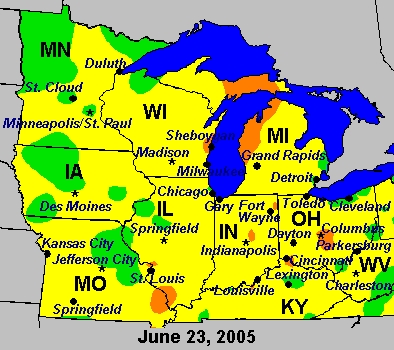
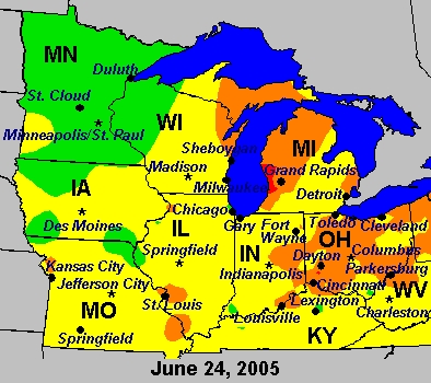
Transport of ozone (and its precursors) is a significant factor and occurs on several spatial
scales. Regionally, over a multi-day period, somewhat stagnant summertime conditions can
lead to the build-up in ozone and ozone precursor concentrations over a large spatial area. This
pollutant air mass can be advected long distances, resulting in elevated ozone levels in
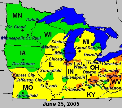
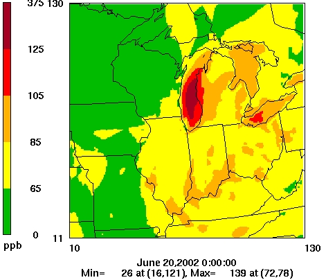
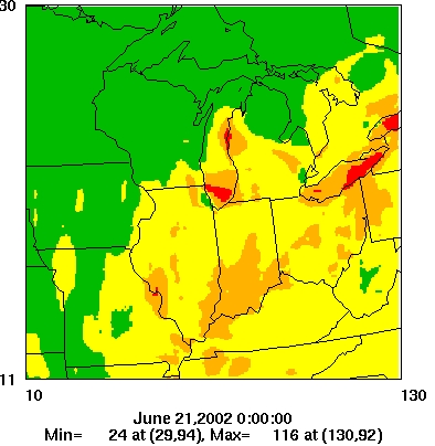
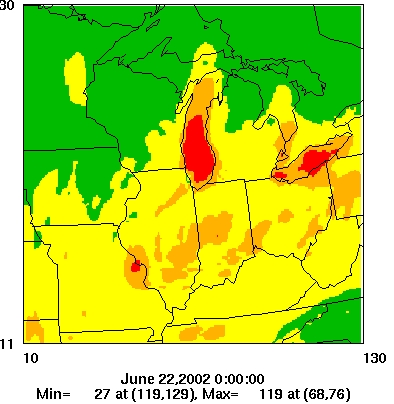
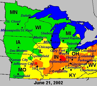
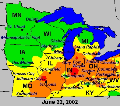
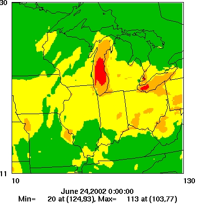
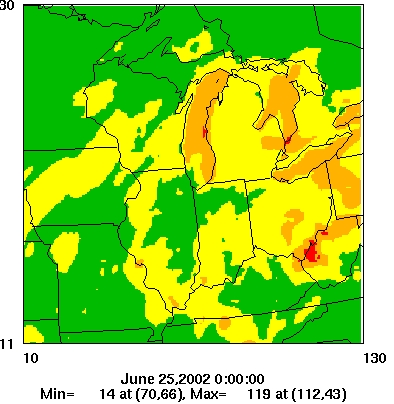
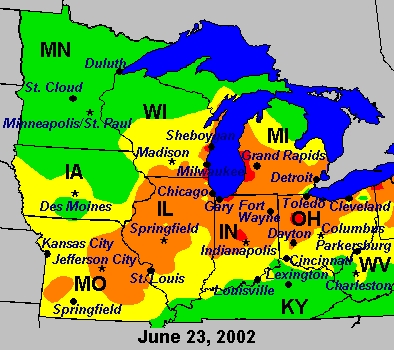
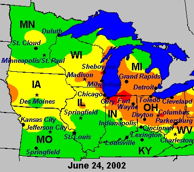
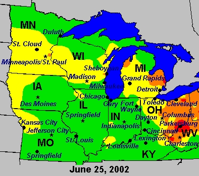
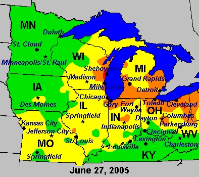
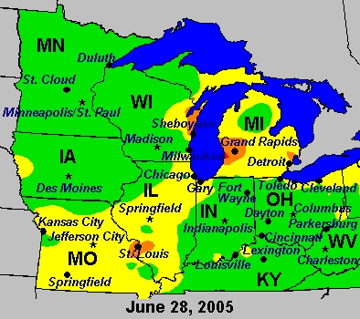
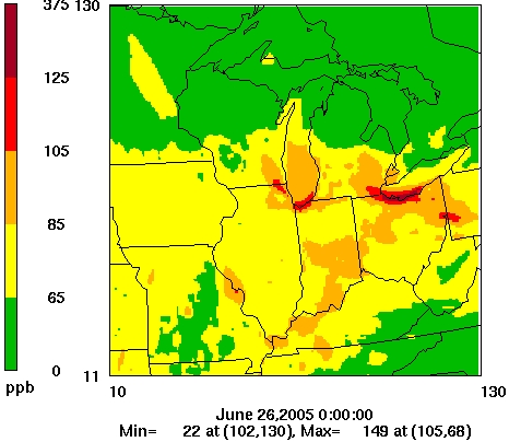
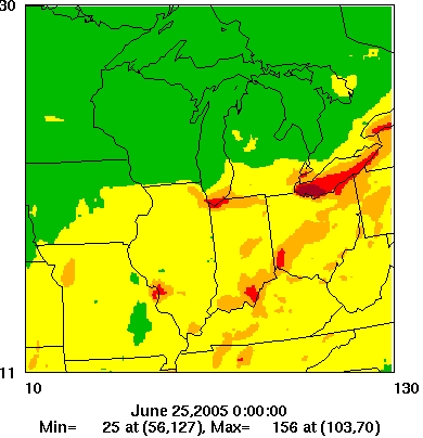
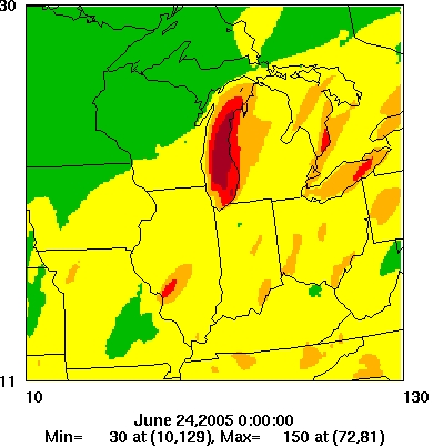
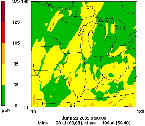
locations far downwind. An example of such an episode is shown in Figure 3.
Figure 3. Example of elevated regional ozone concentrations (June 23 – 25, 2005)
Note: hotter colors represent higher concentrations, with orange representing concentrations above the 8-
hour standard
Electronic Filing - Received, Clerk's Office, January 21, 2009
Appendix A
8
Locally, emissions from urban areas add to the regional background leading to ozone
concentration hot spots downwind. Depending on the synoptic wind patterns (and local land-
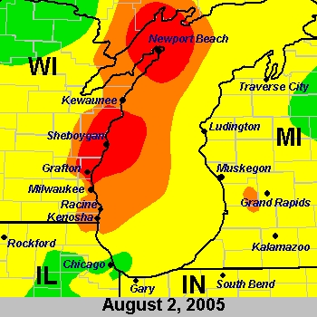
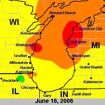
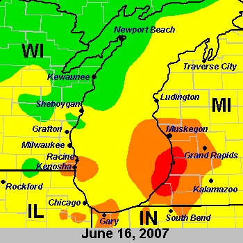
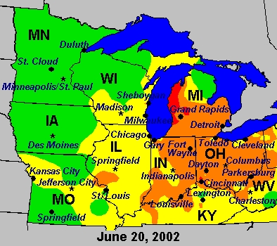
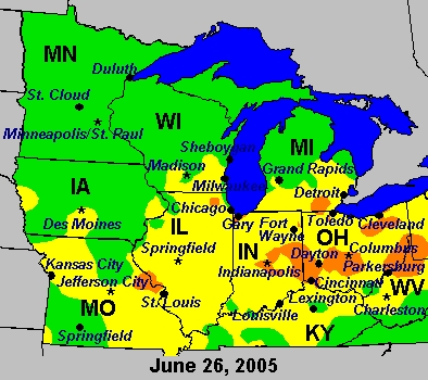
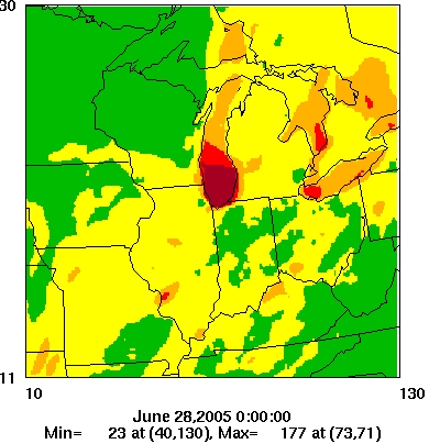
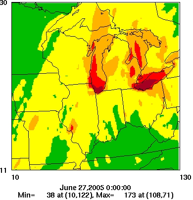
lake breezes), different downwind areas are affected (see, for example, Figure 4).
Figure 4. Examples of recent high ozone days in the Lake Michigan area
Note: hotter colors represent higher concentrations, with orange representing concentrations above the 8-
hour standard
Aloft (aircraft) measurements in the Lake Michigan area also provide evidence of elevated
regional background concentrations and “plumes” from urban areas. For one example summer
day (August 20, 2003 – see Figure 5), the incoming background ozone levels were on the order
of 80 – 100 ppb and the downwind ozone levels over Lake Michigan were on the order of 100 -
150 ppb (STI, 2004).
Figure 5. Aircraft ozone measurements over Lake Michigan (left) and along upwind boundary
(right) – August 20, 2003 (Note: aircraft measurements reflect instantaneous values)
9
As discussed in Section 4, residual nonattainment is projected in at least one area in the 5-state
region –i.e., western Michigan. To understand the source regions likely impacting high ozone
concentrations in western Michigan and estimate the impact of these source regions, two simple
transport-related analyses were performed.
First, back trajectories were constructed using the HYSPLIT model for high ozone days (8-hour
peak > 80 ppb) during the period 2002-2006 in western Michigan to characterize general
transport patterns. Composite trajectory plots for all high ozone days based on data from three
sites (Cass County, Holland, and Muskegon) are provided in Figure 6. The plots point back to
areas located to the south-southwest (especially, northeastern Illinois and northwestern Indiana)
as being upwind on these high ozone days.
Figure 6 Back trajectory analysis showing upwind areas associated with high ozone
concentrations
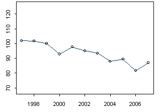
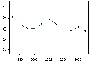
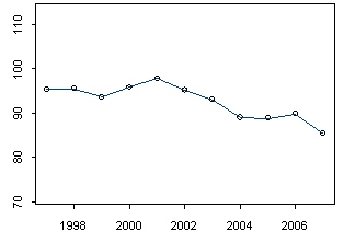
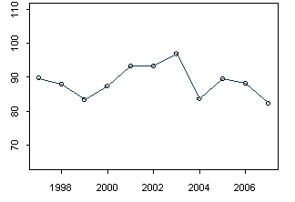
Second, to assess the impact from Chicago/NW Indiana, Blanchard (2005a) compared ozone
concentrations upwind (Braidwood, IL), within Chicago (ten sites in the City), and downwind
(Holland and Muskegon) for days in 1999 – 2002 with southwesterly winds - i.e., transport
towards western Michigan. Figure 7 shows the distribution of daily peak 8-hour ozone
concentrations by day-of-week, with a line connecting the mean values. The difference
between day-of-week mean values at downwind and upwind sites indicates that Chicago/NW
Indiana contributes about 10-15 ppb to downwind ozone levels.
Electronic Filing - Received, Clerk's Office, January 21, 2009
Appendix A
10
Figure 7. Mean day-of-week peak 8-hour ozone concentrations at sites upwind, within, and
downwind of Chicago, 1999 – 2002 (southwesterly wind days)
Based on this information, the following key findings related to transport can be made:
•
Ozone transport is a problem affecting many portions of the eastern U.S. The Lake
Michigan area (and other areas in the LADCO region) both receive high levels of
incoming (transported) ozone and ozone precursors from upwind source areas on many
hot summer days, and contribute to the high levels of ozone and ozone precursors
affecting downwind receptor areas.
•
The presence of a large body of water (i.e., Lake Michigan) influences for the formation
and transport of ozone in the Lake Michigan area. Depending on large-scale synoptic
winds and local-scale lake breezes, different parts of the area experience high ozone
concentrations. For example, under southerly flow, high ozone can occur in eastern
Wisconsin, and under southwesterly flow, high ozone can occur in western Michigan.
•
Downwind shoreline areas around Lake Michigan are affected by both regional transport
of ozone and subregional transport from major cities in the Lake Michigan area.
Counties along the western shore of Michigan (from Benton Harbor to Traverse City, and
even as far north as the Upper Peninsula) are impacted by high levels of incoming
(transported) ozone.
Electronic Filing - Received, Clerk's Office, January 21, 2009
Appendix A
11
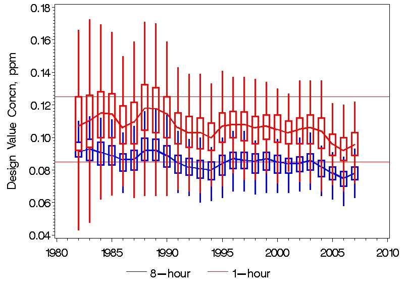
Data Variability:
Since 1980, considerable progress has been made to meet the previous 1-
hour ozone standard. Figure 8 shows the decline in both the 1-hour and 8-hour design values
for the 5-state LADCO region over the last 25 years.
Figure 8 Ozone design value trends in 5-State region
The trend is more dramatic for the higher ozone sites in the 5-state region (see Figure 9). This
plot shows a pronounced downward trend in the design value since the 2001-2003 period, due,
in part, to the very low 4
th
high values in 2004.
Figure 9. Trend in ozone design values and 4
th
high values for higher ozone sites in region
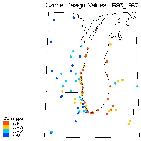
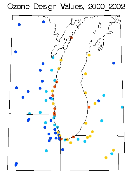
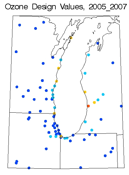
The improvement in ozone concentrations is also seen in the decrease in the number of sites
measuring nonattainment over the past 15 years in the Lake Michigan area (see Figure 10).
75
85
95
105
'95-'97
'96-'98
'97-'99
'98-'00
'99-'01
'00-'02
'01-'03
'02-'04
'03-'05
'04-'06
'05-'07
65
75
85
95
105
115
'95
'96
'97
'98
'99
'00
'01
'02
'03
'04
'05
'06
'07
Design Values
4
th
High Values
Electronic Filing - Received, Clerk's Office, January 21, 2009
Appendix A
12
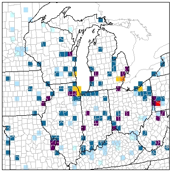
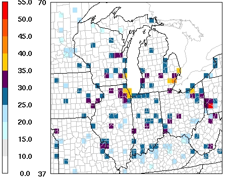
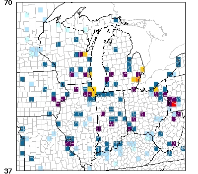
Figure 10. Ozone design value maps for 1995-1997, 2000-2002, and 2005-2007
13
Given the effect of meteorology on ambient ozone levels, year-to-year variations in meteorology
can make it difficult to assess trends in ozone air quality. Two approaches were considered to
adjust ozone trends for meteorological influences: an air quality-meteorology statistical model
developed by EPA (i.e., Cox method), and statistical grouping of meteorological variables
performed by LADCO (i.e., Classification and Regression Trees, or CART).
Cox Method
: This method uses a statistical model to ‘remove’ the annual effect of meteorology
on ozone (Cox and Chu, 1993). A regression model was fit to the 1997-2007 data to relate daily
peak 8-hour ozone concentrations to six daily meteorological variables plus seasonal and
annual factors (Kenski, 2008a). Meteorological variables included were daily maximum
temperature, mid-day average relative humidity, morning and afternoon wind speed and wind
direction. The model is then used to predict 4
th
high ozone values. By holding the
meteorological effects constant, the long term trend can be examined independently of
meteorology. Presumably, any trend reflects changes in emissions of ozone precursors.
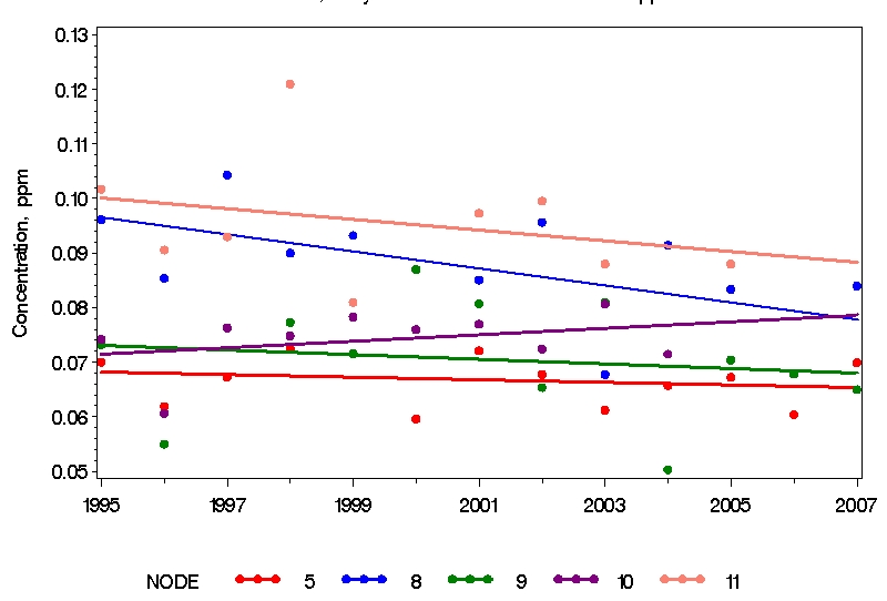
Figure 11a shows the meteorologically-adjusted 4
th
high ozone concentrations for several
monitors near major urban areas in the region. The plots indicate a general downward trend
since the late 1990s for most cities, indicating that recent emission reductions have had a
positive effect in improving ozone air quality.
A similar model was run to examine meteorologically adjusted trends in seasonal average
ozone. This model incorporates more meteorological variables, including rain and long-distance
transport (direction and distance). Model development was documented in Camalier et al.,
2007. The seasonal average trends are shown in Figure 11b. Trends determined by seasonal
model for the same set of sites examined above are consistent with those developed by the 4
th
high model.
14
Chiwaukee, WI
Sheboygan, WI
Cleveland (Ashtabula), OH
Cincinnati (Sycamore), OH
Detroit (New Haven), MI
St. Louis, MO
Indianapolis, IN
Figure 11a. Trends in meteorologically
adjusted 4
th
high 8-hour ozone
concentrations for seven Midwestern sites
(1997 – 2007)
15
Chiwaukee, WI
Sheboygan, WI
1998
2000
2002 2004
2006
20
40
60
80
Seasonal Average
Adjusted
Ozone
for Weather
(ppb)
Unadjusted for Weather
1998
2000
2002
2004
2006
20
40
60
80
Seasonal Average
Adjusted
Ozone
for Weather
(ppb)
Unadjusted for Weather
Cleveland (Ashtabula), OH
Cincinnati (Sycamore), OH
1998
2000
2002
2004
2006
20
40
60
80
Seasonal Average
Adjusted
Ozone
for Weather
(ppb)
Unadjusted for Weather
1998
2000
2002
2004
2006
20
40
60
80
Seasonal Average
Adjusted
Ozone
for Weather
(ppb)
Unadjusted for Weather
Detroit (New Haven), MI
St. Louis, MO
1998
2000
2002 2004
2006
20
40
60
80
Seasonal Average
Adjusted
Ozone
for Weather
(ppb)
Unadjusted for Weather
1998
2000
2002 2004
2006
20
40
60
80
Seasonal Average
Adjusted
Ozone
for Weather
(ppb)
Unadjusted for Weather
Indianapolis, IN
1998
2000
2002 2004
2006
20
40
60
80
Seasonal Average
Adjusted
Ozone
for Weather
(ppb)
Unadjusted for Weather
Figure 11b. Trends in seasonal 8-hour ozone
concentrations for seven Midwestern sites
(1997 – 2007)
16
CART
: Classification and Regression Tree (CART) analysis is another statistical technique
which partitions data sets into similar groups (Breiman et al., 1984). CART analysis was
performed using data for the period 1995-2007 for 22 selected ozone monitors with current 8-
hour design values close to or above the standard (Kenski, 2008b). The CART model searches
through 60 meteorological variables to determine which are most efficient in predicting ozone.
Although the exact selection of predictive variables changes from site to site, the most common
predictors were temperature, wind direction, and relative humidity. Only occasionally were
upper air variables, transport time or distance, lake breeze, or other variables significant. (Note,
the ozone and meteorological data for the CART analysis are the same as used in the EPA/Cox
analysis.)
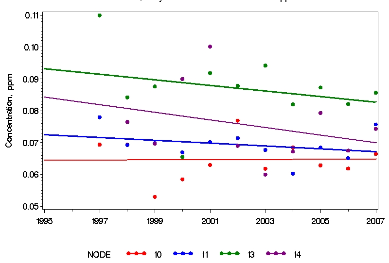
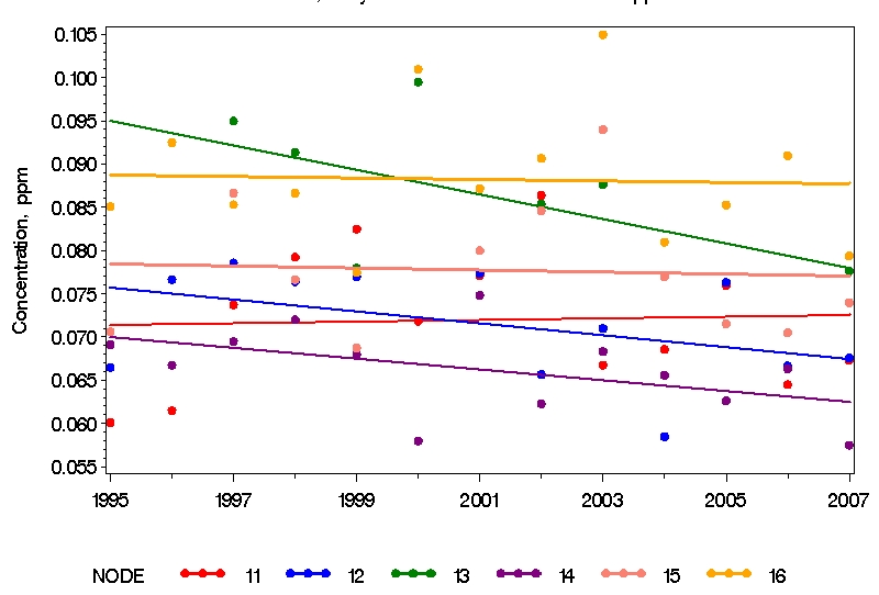
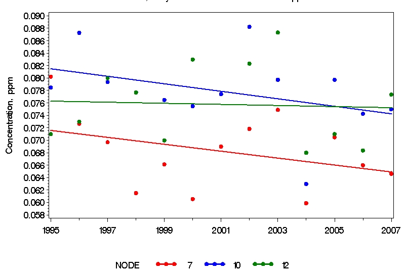
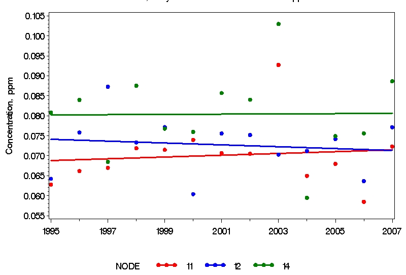
For each monitor, regression trees were developed that classify each summer day (May-
September) by its meteorological conditions. Similar days are assigned to nodes, which are
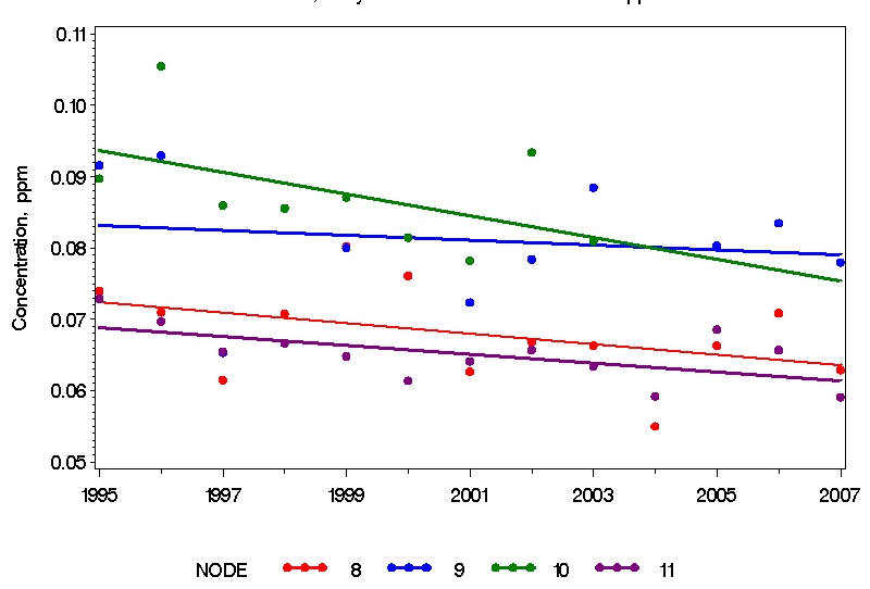
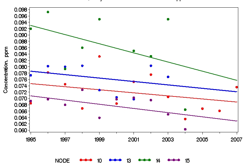
equivalent to branches of the regression tree. Ozone time series for the higher concentration
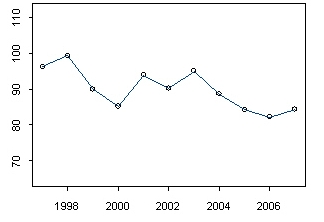
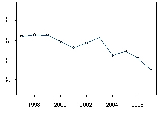
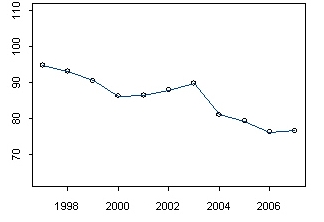
nodes are plotted for select sites in Figure 12. By grouping days with similar meteorology, the
influence of meteorological variability on the trend in ozone concentrations is partially removed;
the remaining trend is presumed to be due to trends in precursor emissions or other non-
meteorological influences. Trends over the 13-year period at most sites were found to be
declining, with the exception of Detroit which showed fairly flat trends. Comparison of the
average of the high concentration node values for 2001-2003 v. 2005-2007 showed an
improvement of about 5 ppb across all sites (even Detroit).
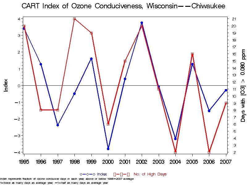
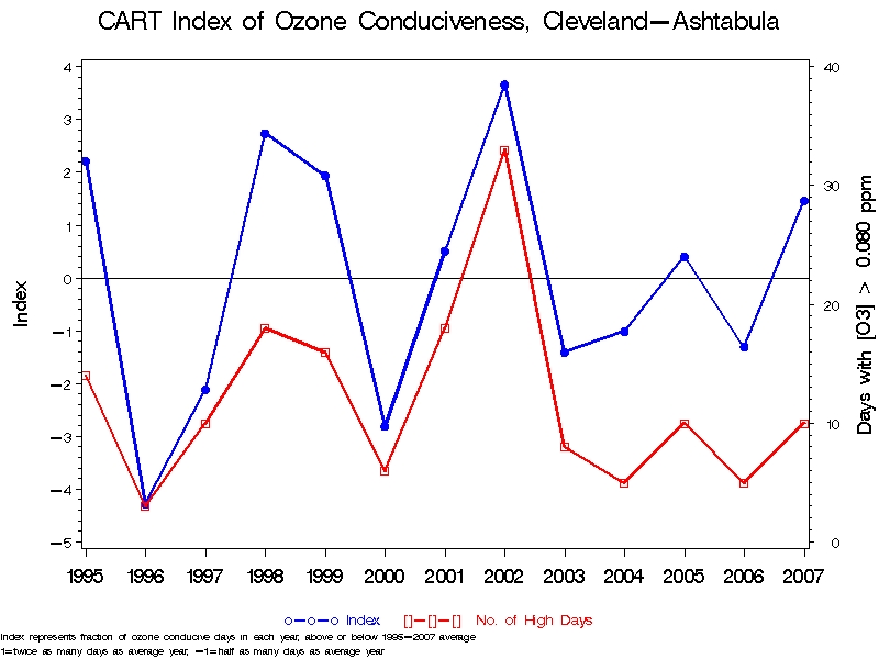
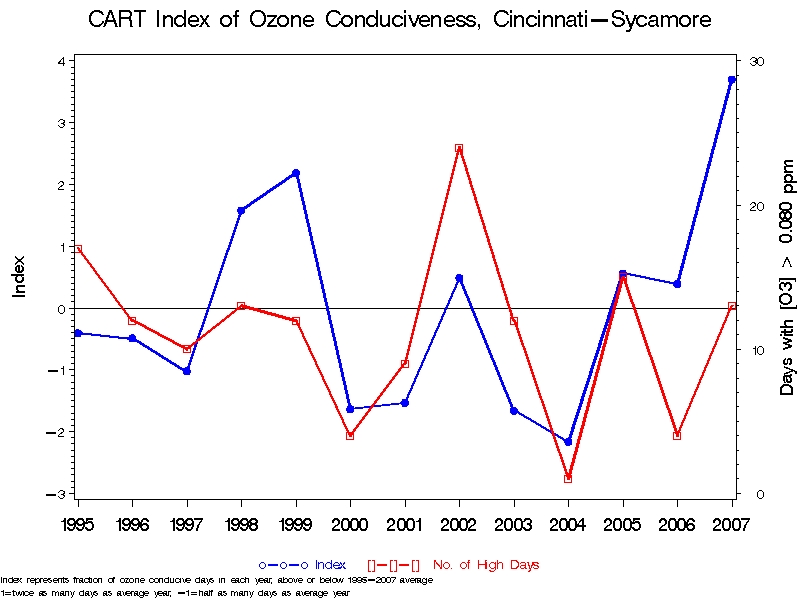
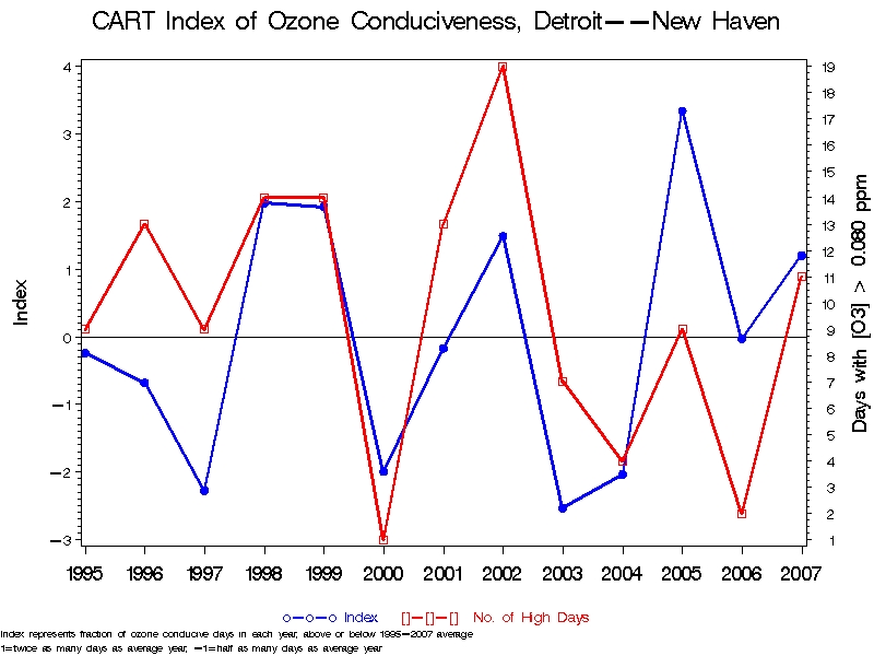
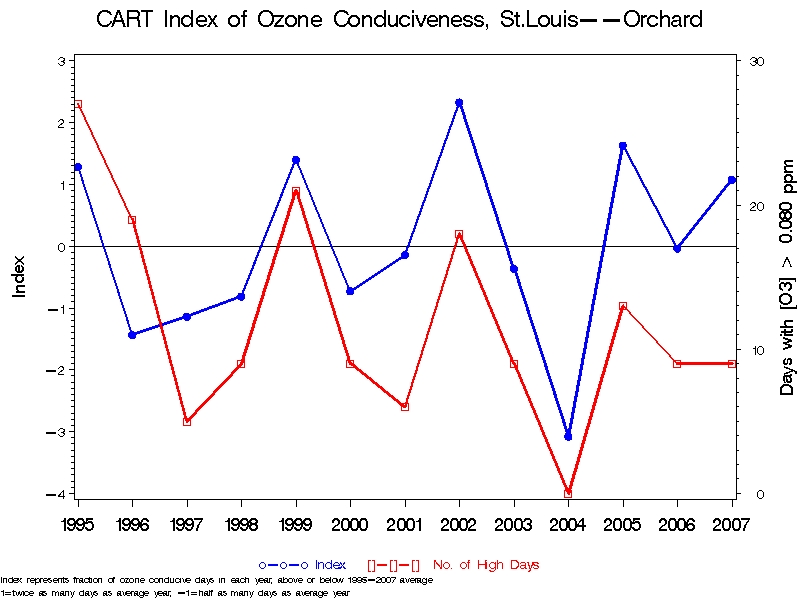
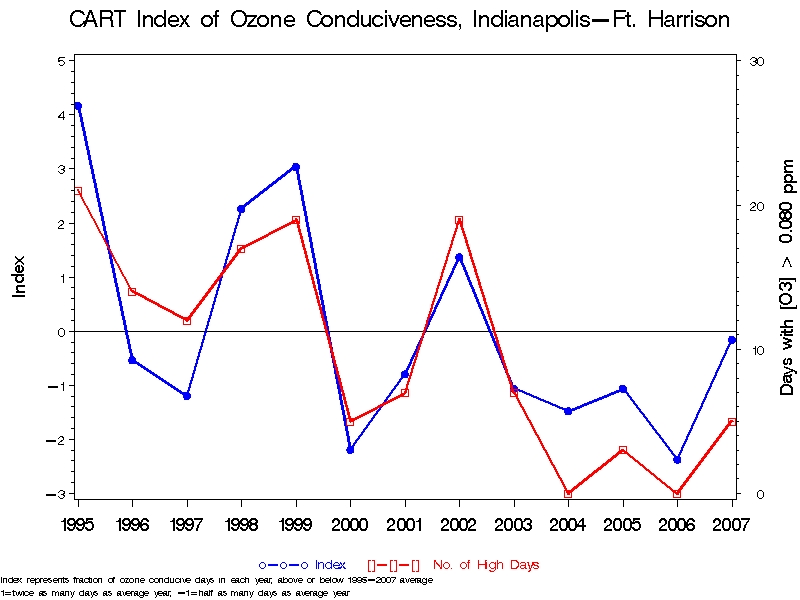
The effect of meteorology was further examined by using an ozone conduciveness index
(Kenski, 2008b). This metric reflects the variability from the 13-year average in the number of
days in the higher ozone concentration nodes (see Figure 13). Examination of these plots
indicates:
•
2002 and 2005 were both above normal, with 2002 tending to be more severe; and
•
2001-2003 and 2005-2007 were both above normal, with no clear pattern in which
period was more severe (i.e., ozone conduciveness values were similar at most sites,
2001-2003 values were higher at a few sites, and 2005-2007 values were higher at a
few sites).
Given the similarity in ozone conduciveness between 2001-2003 and 2005-2007, the
improvement in ozone levels noted above is presumed to be due to non-meteorological factors
(i.e., emission reductions).
In conclusion, all three statistical approaches (CART and the two nonlinear regression models)
show a similar result; ozone in the urban areas of the LADCO region has declined during the
1997-2007 period, even when meteorological variability is accounted for. The decreases are
present whether seasonal average ozone, peak values (annual 4
th
highs), or a subset of high
days with similar meteorology are considered. The consistency in results across models is a
good indication that these trends reflect impacts of emission control programs.
17
Chiwaukee, WI
Sheboygan, WI
Cleveland (Ashtabula), OH
Cincinnati (Sycamore), OH
Detroit (New Haven), MI
St. Louis, MO
Indianapolis, IN
Figure 12. Trends for higher ozone CART
groups (average ozone > 65 ppb) for seven
Midwestern sites (1995 – 2007)
Note: line represents linear best fit
18
Figure 13. Ozone conduciveness index (and
number of high ozone days) for seven
Midwestern site (1995 – 2007)
19
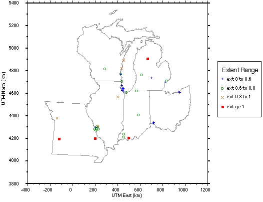
Precursor Sensitivity
: Ozone is formed from the reactions of hydrocarbons and nitrogen oxides
under meteorological conditions that are conducive to such reactions (i.e., warm temperatures
and strong sunlight). In areas with high VOC/NOx ratios, typical of rural environments (with low
NOx), ozone tends to be more responsive to reductions in NOx. Conversely, in areas with low
VOC/NOx ratios, typical of urban environments (with high NOx), ozone tends to be more
responsive to VOC reductions.
An analysis of VOC and NO
x
-limitation was conducted with the ozone MAPPER program, which
is based on the Smog Production (SP) algorithm (Blanchard, et al., 2003). The “Extent of
Reaction” parameter in the SP algorithm provides an indication of VOC and NOx sensitivity:
Extent Range
Precursor Sensitivity
< 0.6
VOC-sensitive
0.6 – 0.8
Transitional
> 0.8
NOx-sensitive
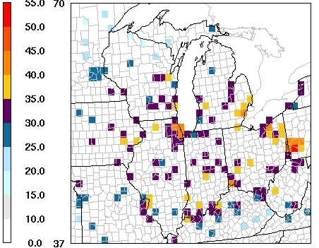
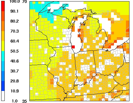
A map of the Extent of Reaction values for high ozone days is provided in Figure 14. As can be
seen, ozone is usually VOC-limited in cities and NOx-limited in rural areas. (Data from aircraft
measurements suggest that ozone is usually NO
x
-limited over Lake Michigan and away from
urban centers on days when ozone in the urban centers is VOC-limited.) The highest ozone
days were found to be NO
x
-limited. This analysis suggests that a NOx reduction strategy would
be effective in reducing ozone levels. Examination of day-of-week concentrations, however,
raises some question about the effectiveness of NOx reductions.
Figure 14. Mean afternoon extent of reaction (1998 – 2002)
Electronic Filing - Received, Clerk's Office, January 21, 2009
Appendix A
20
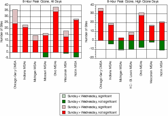
Blanchard (2004 and 2005a) examined weekend-weekday differences in ozone and NO
x
in the
Midwest. All urban areas in these two studies exhibited substantially lower (40-60%) weekend
concentrations of NO
x
compared to weekday concentrations. Despite lower weekend NO
x
concentrations, weekend ozone concentrations were not lower; in fact, most urban sites had
higher concentrations of ozone, although the increase was generally not statistically significant
(see Figure 15). This small but counterproductive change in
local
ozone concentrations
suggests that
local
urban-scale NO
x
reductions alone may not be very effective.
Figure 15. Weekday/weekend differences in 8-hour ozone – number of sites with weekend
increase (positive values) v. number of sites with weekend decreases (negative values)
Two additional analyses, however, demonstrate the positive effect of NOx emission reductions
on downwind ozone concentrations. First, Blanchard (2005a) looked at the effect of changes in
precursor emissions in Chicago on downwind ozone levels in western Michigan. For the
transport days of interest (i.e., southwesterly flow during the summers of 1999 – 2002), mean
NOx concentrations in Chicago are about 50% lower and mean ozone concentrations at the
(downwind) western Michigan sites are about 1.5 – 5.2 ppb (3 – 8 %) lower on Sunday
compared to Wednesday. This degree of change in downwind ozone levels suggests a
positive, albeit non-linear response to urban area emission reductions.
Second, Environ (2007a) examined the effect of differences in day-of-week emissions in
southeastern Michigan on downwind ozone levels. This modeling study found that weekend
changes in ozone precursor emissions cause both increases and decreases in Southeast
Michigan ozone, depending upon location and time:
Electronic Filing - Received, Clerk's Office, January 21, 2009
Appendix A
21
•
Weekend increases in 8-hour maximum ozone occur in and immediately downwind of
the Detroit urban area (i.e., in VOC-sensitive areas).
•
Weekend decreases in 8-hour maximum ozone occur outside and downwind of the
Detroit urban area (i.e., in NOx-sensitive areas).
•
At the location of the peak 8-hour ozone downwind of Detroit, ozone was lower on
weekends than weekdays.
•
Ozone benefits (reductions) due to weekend emission changes in Southeast Michigan
can be transported downwind for hundreds of miles.
•
Southeast Michigan benefits from lower ozone transported into the region on Saturday
through Monday because of weekend emission changes in upwind areas.
In summary, these analyses suggest that urban VOC reductions and regional (urban and rural)
NOx reductions will be effective in lowering ozone concentrations. Local NOx reductions can
lead to local ozone increases (i.e., NOx disbenefits), but this effect does not appear to pose a
problem with respect to attainment of the standard. It should also be noted that urban VOC and
regional NOx reductions are likely to have multi-pollutant benefits (e.g., both lower ozone and
PM
2.5
impacts).
2.2 PM
2.5
In 1997, EPA adopted the PM
2.5
standards of 15 ug/m
3
(annual average) and 65 ug/m3 (24-hour
average). The annual standard is attained if the 3-year average of the annual average PM
2.5
concentration is less than or equal to the level of the standard. The daily standard is attained if
the 98th percentile of 24-hour PM
2.5
concentrations in a year, averaged over three years, is less
than or equal to the level of the standard.
In 2006, EPA revised the PM
2.5
standards to 15 ug/m
3
(annual average) and 35 ug/m
3
(24-hour
average).
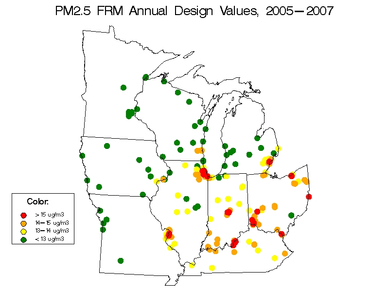
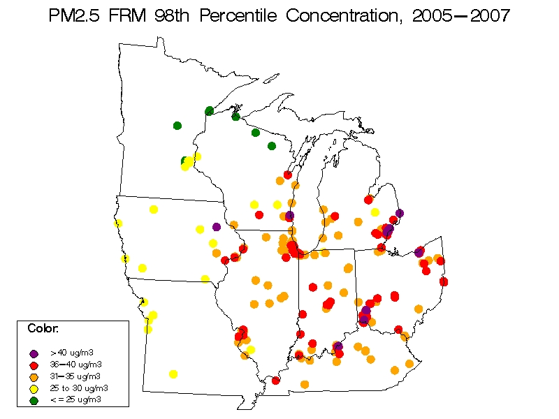
Current Conditions:
Maps of annual and 24-hour PM
2.5
design values for the 3-year period
2005-2007 are shown in Figure 16. The “hotter” colors represent higher concentrations, where
red dots represent sites with design values above the annual standard. Currently, there are 30
sites in violation of the annual PM
2.5
standard.
Table 2 provides the annual PM
2.5
concentrations and associated design values since 2003 for
several high monitoring sites throughout the region.
Electronic Filing - Received, Clerk's Office, January 21, 2009
Appendix A
22
Figure 16. PM
2.5
design values - annual average (top) and 24-hour average (bottom) (2005-2007)
2005 BY
2002 BY
Key Site
County
Site ID
'03
'04
'05
'06
'07
'03 - '05 '04 - '06 '05 - '07
Average
w/ 2007
Average
Chicago - Washington HS
Cook
170310022
15.6 14.2 16.9 13.2 15.7
15.6
14.8
15.3
15.2
15.9
Chicago - Mayfair
Cook
170310052
15.9 15.3 17.0 14.5 15.5
16.1
15.6
15.7
15.8
17.1
Chicago - Springfield
Cook
170310057
15.6 13.8 16.7 13.5 15.1
15.4
14.7
15.1
15.0
15.6
Chicago - Lawndale
Cook
170310076
14.8 14.2 16.6 13.5 14.3
15.2
14.8
14.8
14.9
15.6
Blue Island
Cook
170312001
14.9 14.1 16.4 13.2 14.3
15.1
14.6
14.6
14.8
15.6
Summit
Cook
170313301
15.6 14.2 16.9 13.8 14.8
15.6
15.0
15.2
15.2
16.0
Cicero
Cook
170316005
16.8 15.2 16.3 14.3 14.8
16.1
15.3
15.1
15.5
16.4
Granite City
Madison
171191007
17.5 15.4 18.2 16.3 15.1
17.0
16.6
16.5
16.7
17.3
E. St. Louis
St. Clair
171630010
14.9 14.7 17.1 14.5 15.6
15.6
15.4
15.7
15.6
16.2
Jeffersonville
Clark
180190005
15.8 15.1 18.5 15.0 16.5
16.5
16.2
16.7
16.4
17.2
Jasper
Dubois
180372001
15.7 14.4 16.9 13.5 14.4
15.7
14.9
14.9
15.2
15.5
Gary
Lake
180890031
16.8 13.3 14.5
16.8
15.1
14.9
15.6
Indy - Washington Park
Marion
180970078
15.5 14.3 16.4 14.1 15.8
15.4
14.9
15.4
15.3
16.2
Indy - W 18th Street
Marion
180970081
16.2 15.0 17.9 14.2 16.1
16.4
15.7
16.1
16.0
Indy - Michigan Street
Marion
180970083
16.3 15.0 17.5 14.1 15.9
16.3
15.5
15.8
15.9
16.6
Allen Park
Wayne
261630001
15.2 14.2 15.9 13.2 12.8
15.1
14.4
14.0
14.5
15.8
Southwest HS
Wayne
261630015
16.6 15.4 17.2 14.7 14.5
16.4
15.8
15.5
15.9
17.3
Linwood
Wayne
261630016
15.8 13.7 16.0 13.0 13.9
15.2
14.2
14.3
14.6
15.5
Dearborn
Wayne
261630033
19.2 16.8 18.6 16.1 16.9
18.2
17.2
17.2
17.5
19.3
Wyandotte
Wayne
261630036
16.3 13.7 16.4 12.9 13.4
15.5
14.3
14.2
14.7
16.6
Middleton
Butler
390170003
17.2 14.1 19.0 14.1 15.4
16.8
15.7
16.2
16.2
16.5
Fairfield
Butler
390170016
15.8 14.7 17.9 14.0 14.9
16.1
15.5
15.6
15.8
15.9
Cleveland-28th Street
Cuyahoga
390350027
15.4 15.6 17.3 13.0 14.5
16.1
15.3
14.9
15.4
16.5
Cleveland-St. Tikhon
Cuyahoga
390350038
17.6 17.5 19.2 14.9 16.2
18.1
17.2
16.8
17.4
18.4
Cleveland-Broadway
Cuyahoga
390350045
16.4 15.3 19.3 14.0 15.3
17.0
16.2
16.2
16.5
16.7
Cleveland-E14 & Orange
Cuyahoga
390350060
17.2 16.4 19.4 15.0 15.9
17.7
16.9
16.8
17.1
17.6
Newburg Hts - Harvard Ave Cuyahoga
390350065
15.6 15.2 18.6 13.1 15.8
16.5
15.6
15.8
16.0
16.2
Columbus - Fairgrounds
Franklin
390490024
16.4 15.0 16.4 13.6 14.6
15.9
15.0
14.9
15.3
16.5
Columbus - Ann Street
Franklin
390490025
15.3 14.6 16.4 13.6 14.7
15.4
14.9
14.9
15.1
16.0
Columbus - Maple Canyon Franklin
390490081
14.9 13.6 14.6 12.9 13.1
14.4
13.7
13.5
13.9
16.0
Cincinnati - Seymour
Hamilton
390610014
17.0 15.9 19.8 15.5 16.5
17.6
17.1
17.3
17.3
17.7
Cincinnati - Taft Ave
Hamilton
390610040
15.5 14.6 17.5 13.6 15.1
15.9
15.2
15.4
15.5
15.7
Cincinnati - 8th Ave
Hamilton
390610042
16.7 16.0 19.1 14.9 15.9
17.3
16.7
16.6
16.9
17.3
Sharonville
Hamilton
390610043
15.7 14.9 16.9 14.5 14.8
15.8
15.4
15.4
15.6
16.0
Norwood
Hamilton
390617001
16.0 15.3 18.4 14.4 15.1
16.6
16.0
15.9
16.2
16.3
St. Bernard
Hamilton
390618001
17.3 16.4 20.0 15.9 16.1
17.9
17.4
17.3
17.6
17.3
Steubenville
Jefferson
390810016
17.7 15.9 16.4 13.8 16.2
16.7
15.4
15.5
15.8
17.7
Mingo Junction
Jefferson
390811001
17.3 16.2 18.1 14.6 15.6
17.2
16.3
16.1
16.5
17.5
Ironton
Lawrence
390870010
14.3 13.7 17.0 14.4 15.0
15.0
15.0
15.4
15.2
15.7
Dayton
Montgomery 391130032
15.9 14.5 17.4 13.6 15.6
15.9
15.2
15.5
15.5
15.9
New Boston
Scioto
391450013
14.7 13.0 16.2 14.3 14.0
14.6
14.5
14.8
14.7
17.1
Canton - Dueber
Stark
391510017
16.8 15.6 17.8 14.6 15.9
16.7
16.0
16.1
16.3
17.3
Canton - Market
Stark
391510020
15.0 14.1 16.6 11.9 14.4
15.2
14.2
14.3
14.6
15.7
Akron - Brittain
Summit
391530017
15.4 15.0 16.4 13.5 14.4
15.6
15.0
14.8
15.1
16.4
Akron - W. Exchange
Summit
391530023
14.2 13.9 15.7 12.8 13.7
14.6
14.1
14.1
14.3
15.6
Annual Average Conc.
Design Values
Table 2. PM2.5 Data for Select Sites in 5-State Region
Electronic Filing - Received, Clerk's Office, January 21, 2009
Appendix A
24
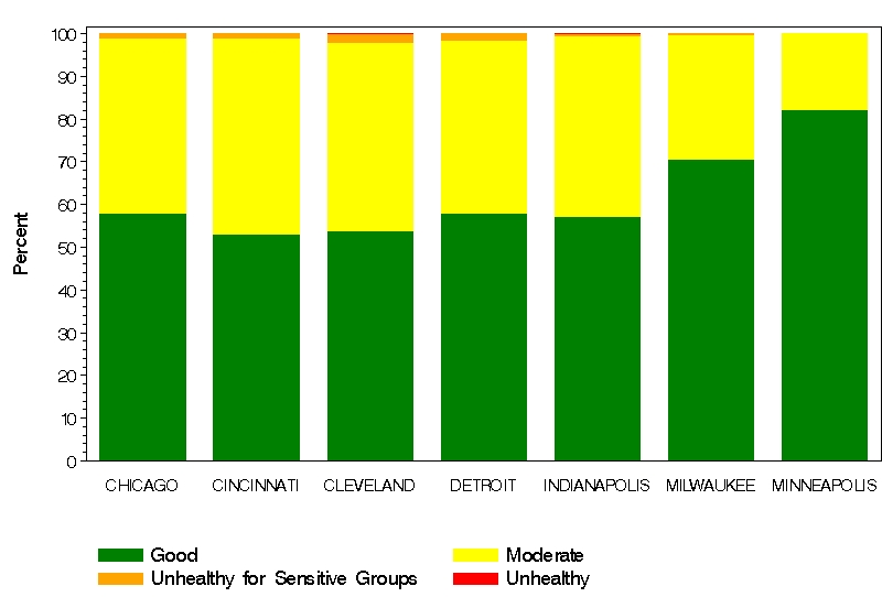
When
EPA initially set the 24-hour standard at 65 μg/m
3
, it also adopted the following
concentration ranges for its Air Quality Index (AQI) scale:
Good
< 15 ug/m
3
Moderate
15-40 μg/m
3
Unhealthy for Sensitive Groups (USG) 40-65 μg/m
3
Unhealthy
65-150 μg/m
3
Figure 17 shows the frequency of these AQI categories for major metropolitan areas in the
region. Daily average concentrations are often in the moderate range and occasionally in the
USG range. Moderate and USG levels can occur any time of the year.
Figure 17. Percent of days in AQI categories for PM
2.5
(2002-2004)
Data Variability
: PM
2.5
concentrations vary spatially, temporally, and chemically in the region.
This variability is discussed further below.
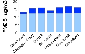
On an annual basis, PM
2.5
exhibits a distinct and consistent spatial pattern. As seen in Figure
16, across the Midwest, annual concentrations follow a gradient from low values (5-6 μg/m
3
) in
northern and western areas (Minnesota and northern Wisconsin) to high values (17-18 μg/m
3
) in
Ohio and along the Ohio River. In addition, concentrations in urban areas are higher than in
upwind rural areas, indicating that local urban sources add a significant increment of 2-3 μg/m
3
to the regional background of 12 - 14 μg/m
3
(see Figure 18).
Figure 18. Regional (lighter shading) v. local components (darker shading) of annual average PM
2.5
concentrations
Electronic Filing - Received, Clerk's Office, January 21, 2009
Appendix A
25
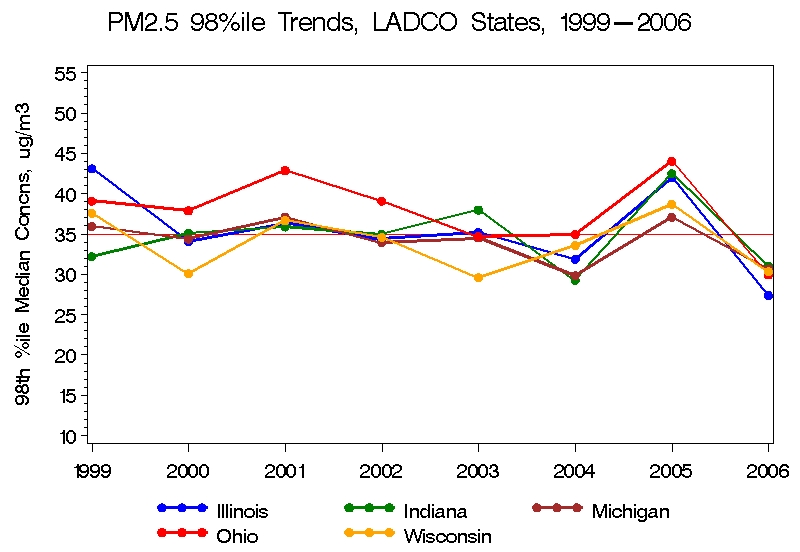
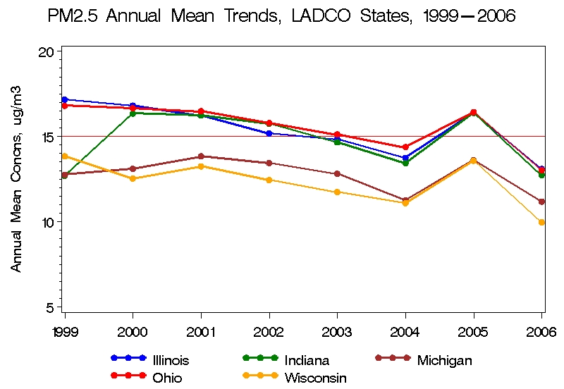
Because monitoring for PM
2.5
only began in earnest in 1999, after promulgation of the PM
2.5
standard, limited data are available to assess trends. Time series based on federal reference
method (FRM) PM
2.5
-mass data show a downward trend in each state (see Figure 19)
7
.
Figure 19. PM
2.5
trends in annual average (top) and daily concentrations (bottom)
7
Despite the general downward trend since 1999, all states experienced an increase during 2005.
Further analyses are underway to understand this increase (e.g., examination of meteorological and
emissions effects).
Electronic Filing - Received, Clerk's Office, January 21, 2009
Appendix A
26
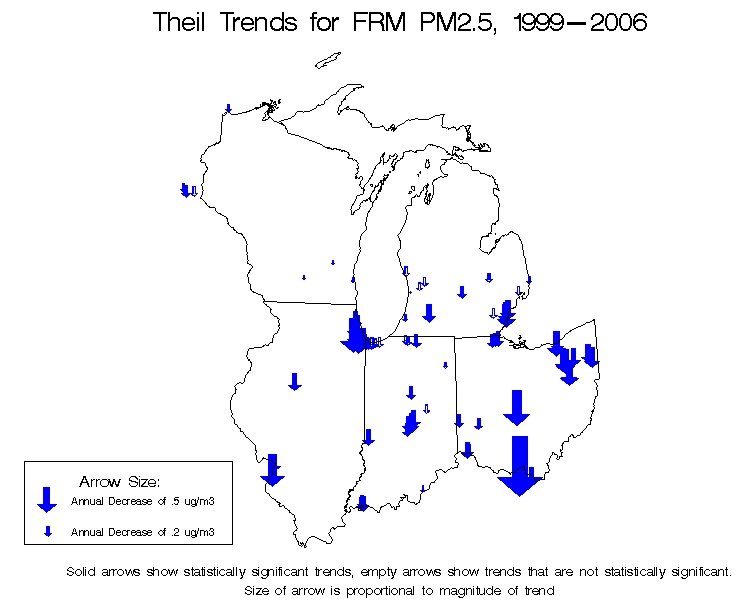
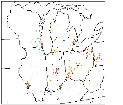
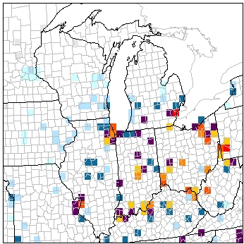
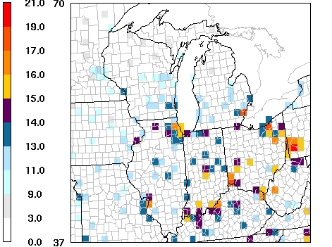
A statistical analysis of PM
2.5
trends was performed using the nonparametric Theil test for slope
(Hollander and Wolfe, 1973). Trends were generally consistent around the region, for both PM
mass and for the individual components of mass. Figure 20 shows trends for PM
2.5
based on
FRM data at sites with six or more years of data since 1999. The size and direction of each
arrow shows the size and direction of the trend for each site; solid arrows show statistically
significant trends and open arrows show trends that are not significant. Region-wide decreases
are widespread and consistent; all sites had decreasing concentration trends (13 of the 38 were
statistically significant). The average decrease for this set of sites is -0.24 ug/m
3
/year.
Figure 20. Annual trends in PM
2.5
mass (1999 – 2006)
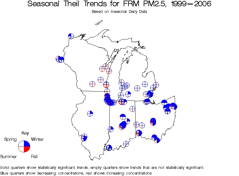
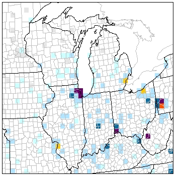
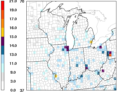
Seasonal trends show mostly similar patterns (Figure 21). Trends were downward at most sites
and seasons, with overall seasonal averages varying between -0.15 to -0.56 ug/m
3
/year. The
strongest and most significant decreases took place during the winter quarter (January - March).
No statistically significant increasing trends were observed.
Electronic Filing - Received, Clerk's Office, January 21, 2009
Appendix A
27
Figure 21. Seasonal trends in PM
2.5
mass (1999 – 2006)
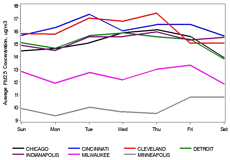
PM
2.5
shows a slight variation from weekday to weekend, as seen in Figure 22. Although most
cities have slightly lower concentrations on the weekend, the difference is usually less than 1
μg/m
3
. There is a more pronounced weekday/weekend difference at monitoring sites that are
strongly source-influenced. Rural monitors tend to show less of a weekday/weekend pattern
than urban monitors.
Figure 22 Day-of-week variability in PM
2.5
(2002-2004)
28
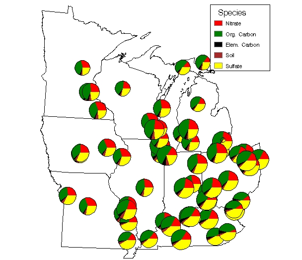
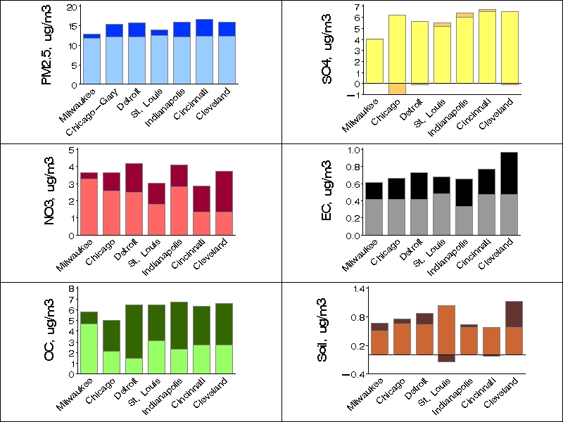
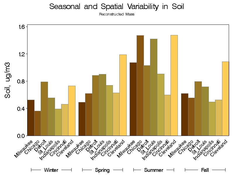
In the Midwest, PM
2.5
is made up of mostly ammonium sulfate, ammonium nitrate, and organic
carbon in approximately equal proportions on an annual average basis. Elemental carbon and
crustal matter (also referred to as soil) contribute less than 5% each.
Figure 23. Spatial map of PM
2.5
chemical composition in the Midwest (2002-2003)
The three major components vary spatially (Figure 23), including notable urban and rural
differences (Figure 24). The components also vary seasonally (Figure 25). These patterns
account for much of the annual variability in PM
2.5
mass noted above.
Figure 24. Average regional (lighter shading) v. local (darker shading) of PM
2.5
chemical species
Electronic Filing - Received, Clerk's Office, January 21, 2009
Appendix A
29
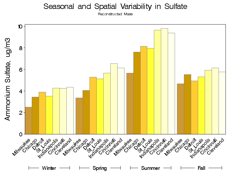
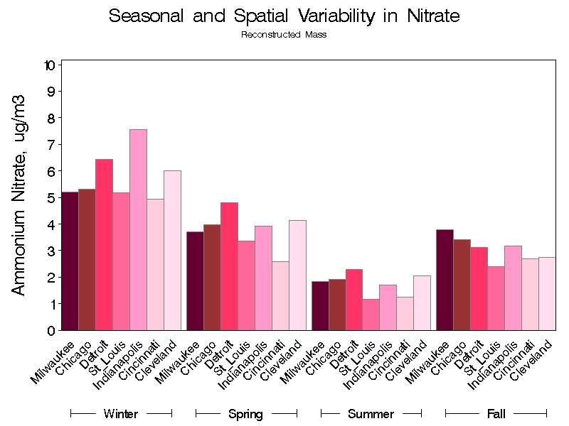
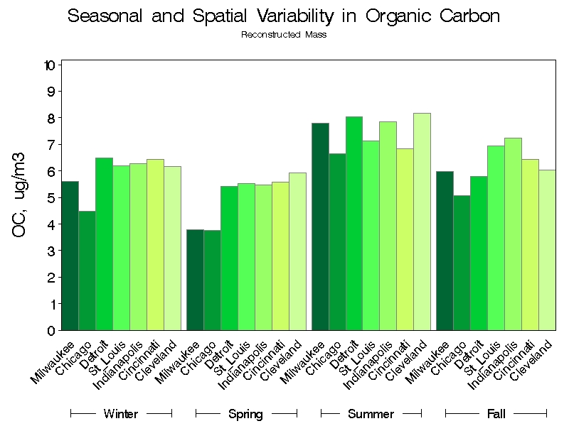
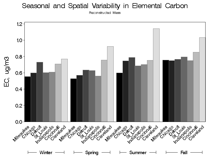
Figure 25 Seasonal and spatial variability in PM
2.5
components
30
Ammonium sulfate peaks in the summer and is highest in the southern and eastern parts of the
Midwest, closest to the Ohio River Valley. Sulfate is primarily a regional pollutant;
concentrations are similar in rural and urban areas and highly correlated over large distances. It
is formed when sulfuric acid (an oxidation product of sulfur dioxide) and ammonia react in the
atmosphere, especially in cloud droplets. Coal combustion is the primary source of sulfur
dioxide; ammonia is emitted primarily from animal husbandry operations and fertilizer use.
Ammonium nitrate has almost the opposite spatial and seasonal pattern, with the highest
concentrations occurring in the winter and in the northern parts of the region. Nitrate seems to
have both regional and local sources, because urban concentrations are higher than rural
upwind concentrations. Ammonium nitrate forms when nitric acid reacts with ammonia, a
process that is enhanced when temperatures are low and humidity is high. Nitric acid is a
product of the oxidation of nitric oxide, a pollutant that is emitted by combustion processes.
Organic carbon is more consistent from season to season and city to city, although
concentrations are generally slightly higher in the summer. Like nitrate, organic carbon has
both regional and local components. Particulate organic carbon can be emitted directly from
cars and other fuel combustion sources or formed in a secondary process as volatile organic
gases react and condense. In rural areas, summer organic carbon has significant contributions
from biogenic sources.
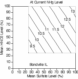
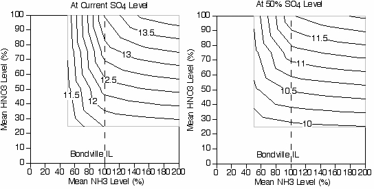
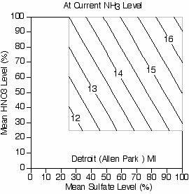
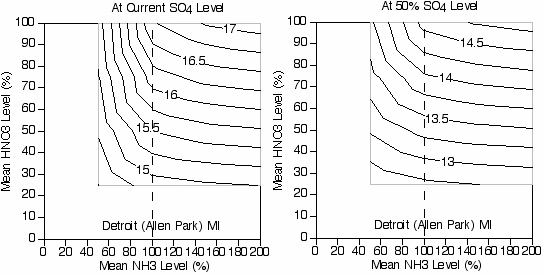
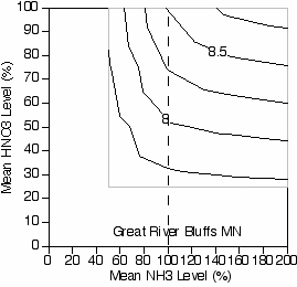
Precursor Sensitivity:
Data from the Midwest ammonia monitoring network were analyzed with
thermodynamic equilibrium models to assess the effect of changes in precursor gas
concentrations on PM
2.5
concentrations (Blanchard, 2005b). These analyses indicate that
particle formation responds in varying degrees to reductions in sulfate, nitric acid, and ammonia.
Based on Figure 26, which shows PM
2.5
concentrations as a function of sulfate, nitric acid
(HNO3), and ammonia (NH3), several key findings should be noted:
•
PM
2.5
mass is sensitive to reductions in sulfate at all times of the year and all parts of the
region. Even though sulfate reductions cause more ammonia to be available to form
ammonium nitrate (PM-nitrate increases slightly when sulfate is reduced), this increase
is generally offset by the sulfate reductions, such that PM
2.5
mass decreases.
•
PM
2.5
mass is also sensitive to reductions in nitric acid and ammonia. The greatest PM
2.5
decrease in response to nitric acid reductions occurs during the winter, when nitrate is a
significant fraction of PM
2.5
.
•
Under conditions with lower sulfate levels (i.e., proxy of future year conditions), PM
2.5
is
more sensitive to reductions in nitric acid compared to reductions in ammonia.
•
Ammonia becomes more limiting as one moves from west to east across the region.
Examination of weekend/weekday difference in PM-nitrate and NOx concentrations in the
Midwest demonstrate that reductions in local (urban) NOx lead to reductions, albeit non-
proportional reductions, in PM-nitrate (Blanchard, 2004). This result is consistent with analyses
of continuous PM-nitrate from several US cities, including St. Louis (Millstein, et al, 2007).
Electronic Filing - Received, Clerk's Office, January 21, 2009
Appendix A
31
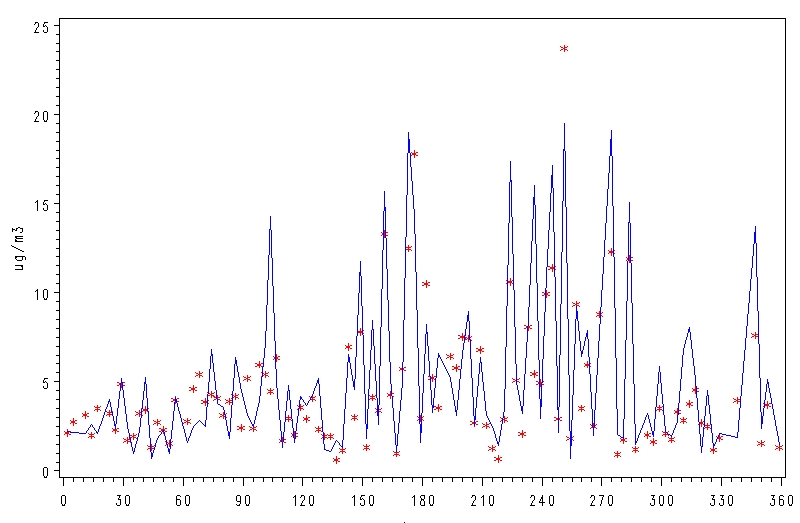
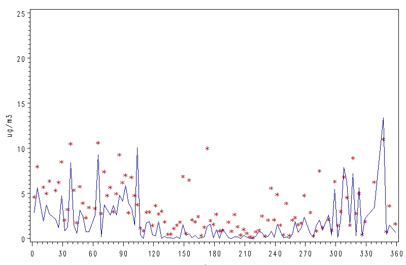
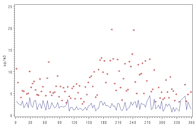
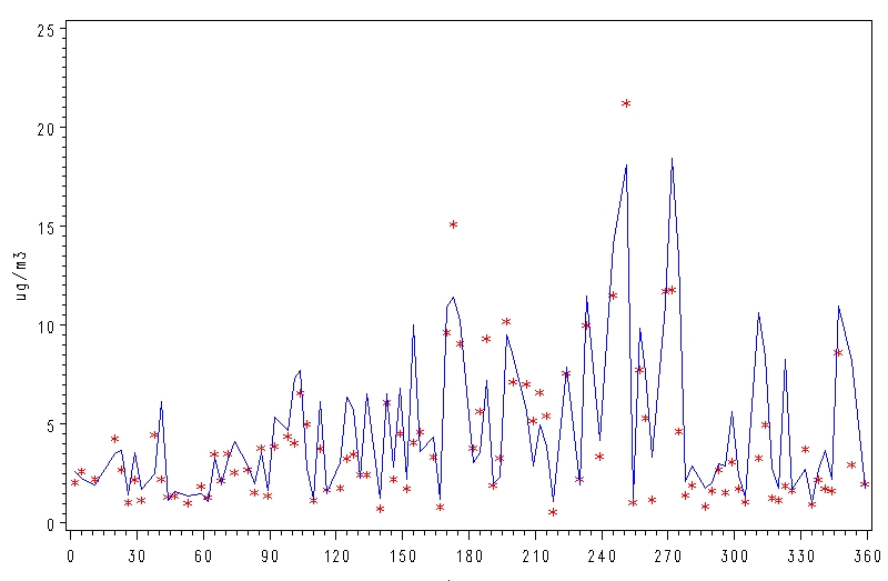
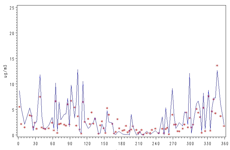
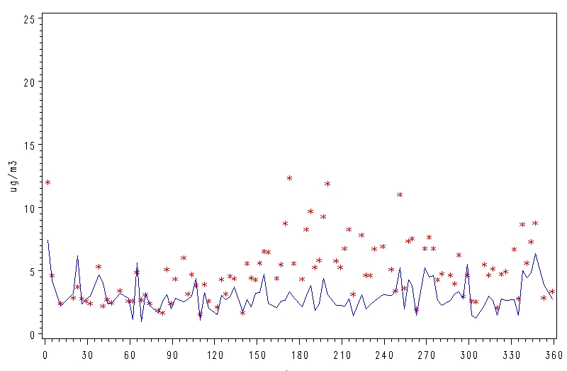
Figure 26. Predicted mean PM fine mass concentrations at Bondville, IL (top) and Detroit (Allen Park), MI
(bottom) as functions of changes in sulfate, nitric acid (HNO3), and ammonia (NH3)
Note: starting at the baseline values (represented by the red star), either moving downward (reductions in nitric
acid) or moving leftward (reductions in sulfate or ammonia) results in lower PM
2.5
values
Electronic Filing - Received, Clerk's Office, January 21, 2009
Appendix A
32
Meteorology
: PM
2.5
concentrations are not as strongly influenced by meteorology as ozone, but
the two pollutants share some similar meteorological dependencies. In the summer, conditions
that are conducive to ozone (hot temperatures, stagnant air masses, and low wind speeds due
to stationary high pressure systems) also frequently give rise to high PM
2.5
. In the case of PM,
the reason is two-fold: (1) stagnation and limited mixing under these conditions cause PM
2.5
to
build up, usually over several days, and (2) these conditions generally promote higher
conversion of important precursors (SO
2
to SO
4
) and higher emissions of some precursors,
especially biogenic carbon. Wind direction is another strong determinant of PM
2.5
; air
transported from polluted source regions has higher concentrations.
Unlike ozone, PM
2.5
has occasional winter episodes. Conditions are similar to those for summer
episodes, in that stationary high pressure and (seasonally) warm temperatures are usually
factors. Winter episodes are also fueled by high humidity and low mixing heights.
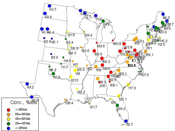
PM
2.5
chemical species show noticeable transport influences. Trajectory analyses have
demonstrated that high PM-sulfate is associated with air masses that traveled through the
sulfate-rich Ohio River Valley (Poirot, et al, 2002 and Kenski, 2004). Likewise, high PM-nitrate
is associated with air masses that traveled through the ammonia-rich Midwest. Figure 27
shows results from an ensemble trajectory analysis of 17 rural eastern IMPROVE sites.
Figure 27. Sulfate and nitrate source regions based on ensemble trajectory analysis
When these results are considered together with analyses of precursor sensitivity (e.g., Figure
26), one possible conclusion is that ammonia control in the Midwest could be effective at
reducing nitrate concentrations. The thermodynamic equilibrium modeling shows that ammonia
reductions would reduce PM concentrations in the Midwest, but that nitric acid reductions are
more effective when the probable reductions in future sulfate levels are considered.
Electronic Filing - Received, Clerk's Office, January 21, 2009
Appendix A
33
Source Culpability:
Three source apportionment studies were performed using speciated PM
2.5
monitoring data and statistical analysis methods (Hopke, 2005, STI, 2006, and STI, 2008).
Figure 28 summarizes the source contributions from these studies. The studies show that a
large portion of PM
2.5
mass consists of secondary, regional impacts, which cannot be attributed
to individual facilities or sources (e.g., secondary sulfate, secondary nitrate, and secondary
organic aerosols). Nevertheless, wind analyses (e.g., Figure 27) provide information on likely
source regions. Regional- or national-scale control programs may be the most effective way to
deal with these impacts. EPA's CAIR, for example, will provide for substantial reductions in
SO2 emissions over the eastern half of the U.S., which will reduce sulfate (and PM
2.5
)
concentrations and improve visibility levels.
The studies also show that a smaller, yet significant portion of PM
2.5
mass is due to emissions
from nearby (local) sources. Local (urban) excesses occur in many urban areas for organic and
elemental carbon, crustal matter, and, in some cases, sulfate. The statistical analysis methods
help to identify local sources and quantify their impact. This information is valuable to states
wishing to develop control programs to address local impacts. A combination of
national/regional-scale and local-scale emission reductions may be necessary to provide for
attainment.
The carbon sources are not easily identified in complex urban environments. LADCO’s Urban
Organics Study (STI, 2006) identified four major sources of organic carbon: mobile sources,
burning, industrial sources, and secondary organic aerosols. Additional sampling and analysis
is underway in Cleveland and Detroit to provide further information on sources of organic
carbon.
Electronic Filing - Received, Clerk's Office, January 21, 2009
Appendix A
34
0
1
2
3
4
5
6
7
Coal
Combustion
Secondary
Nitrate
Mobile
Industrial
Soil
Burning
ug/m3
Northbrook (Jan 03-Mar 05)
Cincinnati (Dec 03-Mar 05)
Indianapolis (Jan 02-Mar 05)
Allen Park (2002-2004)
Dearborn (Jun 02-May 05)
Bondville (2002-2004)
St. Louis (2004)
Granite City (2002-2004)
Tikhon (Jan 03-Jun05)
Orange (Apr 01-Mar 05)
Lorain (Feb 02-Dec04)
0
2
4
6
8
10
sulfate
nitrate
OM
diesel
soil
steel
ind. zinc
ind. copper
mixed ind.
Allen Park
Dearborn
Lawndale
Springfield
Tikhon
Craig
Taft
Figure 28. Major Source Contributions in the Midwest based on Hopke, 2005 (upper left), STI, 2006 (upper right), and STI, 2008 (lower left)
(Note: the labeling of similar source types varies between studies – e.g., organic carbon/mobile sources are named gasoline and diesel by
Hopke, mobile by STI 2006, and OM and diesel by STI 2008)
Electronic Filing - Received, Clerk's Office, January 21, 2009
Appendix A
35
2.3 Haze
Section 169A of the Clean Air Act sets as a national goal “the prevention of any future, and the
remedying of any existing, impairment of visibility in mandatory Class I Federal areas which
impairment results from manmade air pollution”. To implement this provision, in 1999, EPA
adopted regulations to address regional haze visibility impairment (USEPA, 1999). EPA’s rule
requires states to “make reasonable progress toward meeting the national goal”. Specifically,
states must establish reasonable progress goals, which provide for improved visibility on the
most impaired (20% worst) days sufficient to achieve natural conditions by the year 2064, and
for no degradation on the least impaired (20% best) days.
The primary cause of impaired visibility in the Class I areas is pollution by fine particles that
scatter light. The degree of impairment, which is expressed in terms of visual range, light
extinction (1/Mm), or deciviews (dv), depends not just on the total PM
2.5
mass concentration, but
also on the chemical composition of the particles and meteorological conditions.
Current Conditions
: A map of the average light extinction values for the most impaired (20%
worst) visibility days for the 5-year baseline period (2000-2004) is shown in Figure 29.
Figure 29. Baseline Visibility Levels for 20% Worst Days (2000 – 2004), units: Mm
-1
Electronic Filing - Received, Clerk's Office, January 21, 2009
Appendix A
36
Initially, the baseline (2000 – 2004) visibility condition values were derived using the average for
the 20% worst and 20% best days for each year, as reported on the VIEWS website:
http://vista.cira.colostate.edu/views/Web/IMPROVE/SummaryData.aspx . These values were
calculated using the original IMPROVE equation for reconstructed light extinction.
Three changes were made to the baseline calculations to produce a new set of values. First,
the reconstructed light extinction equation was revised by the IMPROVE Steering Committee in
2005. The new IMPROVE equation was used to calculate updated baseline values.
Second, due to sampler problems, the 2002-2004 data for Boundary Waters were invalid for
certain chemical species. (Note, sulfate and nitrate data were valid.) A “substituted” data set
was developed by using values from Voyageurs for the invalid species.
Third, LADCO identified a number of days during 2000-2004 where data capture at the Class I
monitors was incomplete (Kenski, 2007b). The missing data cause these days to be excluded
from the baseline calculations. However, the light extinction due to the remaining measured
species is significant (i.e., above the 80
th
percentile). It makes sense to include these days in
the baseline calculations, because they are largely dominated by anthropogenic sources. (Only
one of these days is driven by high organic carbon, which might indicate non-anthropogenic
aerosol from wildfires.) As seen in Table 3, inclusion of these days in the baseline calculation
results in a small, but measurable, effect on the baseline values (i.e., values increase from 0.2
to 0.8 dv).
Table 3. Average of 20% worst days, with and without missing data days
Average Worst Day
DV, per RHR
Average Worst Day DV,
with Missing Data Days
Difference
BOWA
19.59
19.86
0.27
ISLE
20.74
21.59
0.85
SENE
24.16
24.38
0.22
VOYA
19.27
19.48
0.21
A summary of the initial and updated baseline values for the Class I areas in northern Michigan
and northern Minnesota are presented in Table 4. The updated baseline values reflect the most
current, complete understanding of visibility impairing effects and, as such, will be used for SIP
planning purposes.
Electronic Filing - Received, Clerk's Office, January 21, 2009
Appendix A
37
Table 4. Summary of visibility metrics (deciviews) for northern Class I areas
Old IMPROVE Equation (Cite: VIEWS, November 2005)
20% Worst Days
2000
2001
2002
2003
2004
Baseline
Value
2018
URI Value
Natural
Conditions
Voyageurs
18.50
18.00
19.00
19.20
17.60
18.46
16.74
11.09
BWCA
19.85
19.99
19.68
19.73
17.65
19.38
17.47
11.21
Isle Royale
20.00
22.00
20.80
19.50
19.10
20.28
18.17
11.22
Seney
22.60
24.90
24.00
23.80
22.60
23.58
20.73
11.37
20% Best Days
2000
2001
2002
2003
2004
Baseline
Value
Natural
Conditions
Voyageurs
6.30
6.20
6.70
7.00
5.40
6.32
3.41
BWCA
5.90
6.52
6.93
6.67
5.61
6.33
3.53
Isle Royale
5.70
6.40
6.40
6.30
5.30
6.02
3.54
Seney
5.80
6.10
7.30
7.50
5.80
6.50
3.69
New IMPROVE Equation (Cite: VIEWS, March 2006)
20% Worst Days
2000
2001
2002
2003
2004
Baseline
Value
2018
URI Value
Natural
Conditions
Voyageurs
19.55
18.57
20.14
20.25
18.87
19.48
17.74
12.05
BWCA
20.20
20.04
20.76
20.13
18.18
19.86
17.94
11.61
Isle Royale
20.53
23.07
21.97
22.35
20.02
21.59
19.43
12.36
Seney
22.94
25.91
25.38
24.48
23.15
24.37
21.64
12.65
20% Best Days
2000
2001
2002
2003
2004
Baseline
Value
Natural
Conditions
Voyageurs
7.01
7.12
7.53
7.68
6.37
7.14
4.26
BWCA
6.00
6.92
7.00
6.45
5.77
6.43
3.42
Isle Royale
6.49
7.16
7.07
6.99
6.12
6.77
3.72
Seney
6.50
6.78
7.82
8.01
6.58
7.14
3.73
Notes: (1) BWCA values for 2002 - 2004 reflect "substituted" data.
(2) New IMPROVE equation values include Kenski, 2007 adjustment for missing days
URI = uniform rate of improvement
38
As noted above, the goal of the visibility program is to achieve natural conditions. Initially, the
natural conditions values for each Class I area were taken directly from EPA guidance (EPA,
2003). These values were calculated using the original IMPROVE equation. This equation was
revised by the IMPROVE Steering Committee in 2005, and the new IMPROVE equation was
used to calculate updated natural conditions values. The updated values are reported on the
VIEWS website.
A summary of the initial and updated natural conditions values are presented in Table 4. The
updated natural conditions values (based on the new IMPROVE equation) will be used for SIP
planning purposes.
Data Variability:
For the four northern Class I areas, the most important PM
2.5
chemical species
are ammonium sulfate, ammonium nitrate, and organic carbon. The contribution of these
species on the 20% best and 20% worst visibility days (based on 2000 – 2004 data) is provided
in Figure 30. For the 20% worst visibility days, the contributions are: sulfate = 35-55%, nitrate =
25-30%, and organic carbon = 12-22%. Although the chemical composition is similar, sulfate
increases in importance from west to east and concentrations are highest at Seney (the
easternmost site). It should also be noted that sulfate and nitrate contribute more to light
extinction than to PM
2.5
mass because of their hygroscopic properties.
20% Best Days
20% Worst Days
0
20
40
60
80
100
120
VOYA BOWA ISRO Seney
VOYA BOWA ISRO Seney
sea salt
soil
elem. carbon
coarse mass
organic carbon
nitrate
sulfate
Figure 30. Chemical composition of light extinction for 20% best visibility days (left) and 20%
worst visibility days (right) in terms of Mm
-1
Analysis of PM
2.5
mass and chemical species for rural IMPROVE (and IMPROVE-protocol) sites
in the eastern U.S. showed a high degree of correlation between PM
2.5
-mass, sulfate, and
nitrate levels (see Figure 31). The Class I sites in northern Michigan and northern Minnesota, in
particular, are highly correlated for PM
2.5
mass, sulfates, and organic carbon mass (AER, 2004).
Electronic Filing - Received, Clerk's Office, January 21, 2009
Appendix A
39
Figure 31. Correlations among IMPROVE (and IMPROVE-protocol) monitoring sites in Eastern U.S.
Long-term trends at Boundary Waters (the only regional site with a sufficient data record) show
significant decreases in total PM
2.5
(-0.005 ug/year) and SO4 (-0.04 ug/year) and an increase in
NO3 (+0.01 ug/year). These PM
2.5
and SO4 trends are generally consistent with long-term
trends at other IMPROVE sites in the eastern U.S., which have shown widespread decreases in
SO4 and PM
2.5
(DeBell, et al, 2006). Detecting changes in nitrate has been hampered by
uncertainties in the IMPROVE data for particular years and, thus, this estimate should be
considered tentative.
Haze in the Midwest Class I areas has no strong seasonal pattern. Poor visibility days occur
throughout the year, as indicated in Figure 32. (Note, in contrast, other parts of the country,
such as Shenandoah National Park in Virginia, show a strong tendency for the worst air quality
days to occur in the summer months.) This figure and Figure 33 (which presents the monthly
average light extinction values based on all sampling days) also show that sulfate and organic
carbon concentrations are higher in the summer, and nitrate concentrations are higher in the
winter, suggesting the importance of different sources and meteorological conditions at different
times of the year.
Electronic Filing - Received, Clerk's Office, January 21, 2009
Appendix A
40
Figure 32. Daily light extinction values for 20% worst days at Boundary Waters (2000 – 2004)
41
Figure 33. Monthly average light extinction values for northern Class I areas
Electronic Filing - Received, Clerk's Office, January 21, 2009
Appendix A
42
Precursor Sensitivity:
Results from two analyses using thermodynamic equilibrium models
provide information on the effect of changes in precursor concentrations on PM
2.5
concentrations (and, in turn, visibility levels) in the northern Class I areas. First, a preliminary
analysis using data collected at Seney indicated that PM
2.5
there is most sensitive to reductions
in sulfate, but is also sensitive to reductions in nitric acid (Blanchard, 2004).
Second, an analysis was performed using data from the Midwest ammonia monitoring network
for a site in Minnesota -- Great River Bluffs, which is the closest ammonia monitoring site to the
northern Class I areas (Blanchard, 2005b). Figure 34 shows PM
2.5
concentrations as a function
of sulfate, nitric acid (HNO3), and ammonia (NH3). Reductions in sulfate (i.e., movement to the
left of baseline value [represented by the red star]), as well as reductions in nitric acid (i.e.,
movement downward) and NH3 (i.e., movement to the left), result in lower PM
2.5
concentrations.
Thus, reductions in sulfate, nitric acid, and ammonia will lower PM
2.5
concentrations and
improve visibility in the northern Class I areas.
Figure 34. Predicted PM
2.5
mass concentrations at Great River Bluffs, MN as functions of changes
in sulfate, nitric acid, and ammonia
Meteorology and Transport:
The role of meteorology in haze is complex. Wind speed and wind
direction govern the movement of air masses from polluted areas to the cleaner wilderness
areas. As noted above, increasing humidity increases the efficiency with which sulfate and
nitrate aerosols scatter light. Temperature and humidity together govern whether ammonium
nitrate can form from its precursor gases, nitric acid and ammonia. Temperature and sunlight
also play an indirect role in emissions of biogenic organic species that condense to form
particulate organic matter; emissions increase in the summer daylight hours.
Trajectory analyses were performed to understand transport patterns for the 20% worst and
20% best visibility days. The composite results for the four northern Class I areas are provided
in Figure 35. The orange areas are where the air is most likely to come from, and the green
areas are where the air is least likely to come from. As can be seen, bad air days are generally
associated with transport from regions located to the south, and good air days with transport
from Canada.
43
Figure 35. Composite back trajectories for light extinction- 20% best visibility days (left) and
20% worst visibility days (right) (2000 – 2005)
Source Culpability:
Air quality data analyses (including the trajectory analyses above) and
dispersion modeling were used to provide information on source region and source sector
contributions to regional haze in the northern Class I areas (see MRPO, 2008). Based on this
information, the most important contributing states are Michigan, Minnesota, and Wisconsin, as
well as Missouri, North Dakota, Iowa, Indiana and Illinois (see, for example, Figure 35 above).
The most important contributing pollutants and source sectors are SO2 emissions from
electrical generating units (EGUs) and certain non-EGUs, which lead to sulfate formation, and
NOx emissions from a variety of source types (e.g., motor vehicles), which lead to nitrate
formation. Ammonia emissions from livestock waste and fertilizer applications are also
important, especially for nitrate formation.
A source apportionment study was performed using monitoring data from Boundary Waters and
statistical analysis methods (DRI, 2005). The study shows that a large portion of PM
2.5
mass
consists of secondary, regional impacts, which cannot be attributed to individual facilities or
sources (e.g., secondary sulfate, secondary nitrate, and secondary organic aerosols). Industrial
sources contribute about 3-4% and mobile sources about 4-7% to PM
2.5
mass.
A special study was performed in Seney to identify sources of organic carbon (Sheesley, et al,
2004). As seen in Figure 36, the highest PM
2.5
concentrations occurred during the summer,
with organic carbon being the dominant species. The higher summer organic carbon
concentrations were attributed mostly to secondary organic aerosols of biogenic origin because
of the lack of primary emission markers, and concentrations of know biogenic-related species
(e.g., pinonic acid – see Figure 36) were also high during the summer.
44
Figure 36. Monthly concentrations of PM
2.5
species (top), and secondary and biogenic-related
organic carbon species in Seney (bottom)
45
Although the Seney study showed that biomass burning was a relatively small contributor to
organic carbon on an annual average basis, episodic impacts are apparent (see, for example,
high organic carbon days in Figure 32). To assess further whether burning is a significant
contributor to visibility impairment in the northern Class I areas, the PM
2.5
chemical speciation
data were examined for days with high organic carbon and elemental carbon concentrations,
which are indicative of biomass burning impacts. Only a handful of such days were identified:
Table 5. Days with high OC and EC concentrations in northern Class I areas
Site
2000
2001
2002
2003
2004
Voyageurs
---
---
Jun 1
Aug 25
Jul 17
Jun 28
Jul 19
Boundary Waters
---
---
Jun 28
Aug 25
Jul 17
Jul 19
Isle Royale
---
---
Jun 1
Aug 25
---
Jun 28
Seney
---
---
Jun 28
---
---
Back trajectories on these days point mostly to wildfires in Canada. Elimination of these high
organic carbon concentration days has a small effect in lowering the baseline visibility levels in
the northern Class I areas (i.e., Minnesota Class I areas change by about 0.3 deciviews and
Michigan Class I areas change by less than 0.2 deciviews). This suggests that fire activity,
although significant on a few days, is on average a relatively small contributor to visibility
impairment in the northern Class I areas.
In summary, these analyses show that organic carbon in the northern Class I is largely
uncontrollable.
46
Section 3.0 Air Quality Modeling
Air quality models are relied on by federal and state regulatory agencies to support their
planning efforts. Used properly, models can assist policy makers in deciding which control
programs are most effective in improving air quality, and meeting specific goals and objectives.
For example, models can be used to conduct “what if” analyses, which provide information for
policy makers on the effectiveness of candidate control programs.
The modeling analyses were conducted in accordance with EPA’s modeling guidelines (EPA,
2007a). Further details of the modeling are provided in two protocol documents: LADCO, 2007a
and LADCO, 2007b.
This section reviews the development and evaluation of the modeling system used for the multi-
pollutant analyses. Application of the modeling system (i.e., attainment demonstration for ozone
and PM
2.5
, and reasonable progress assessment for haze) is covered in the following sections.
3.1 Selection of Base Year
Two base years were used in the modeling analyses: 2002 and 2005. EPA’s modeling
guidance recommends using 2002 as the baseline inventory year, but also allows for use of an
alternative baseline inventory year, especially a more recent year. Initially, LADCO conducted
modeling with a 2002 base year (i.e., Base K/Round 4 modeling, which was completed in 2006).
A decision was subsequently made to conduct modeling with a 2005 base year (i.e., Base
M/Round 5, which was completed in 2007). As discussed in the previous section, 2002 and
2005 both had above normal ozone conducive conditions, although 2002 was more severe
compared to 2005. Examination of multiple base years provides for a more complete technical
assessment. Both sets of model runs are discussed in this document.
3.2 Future Years of Interest
To address the multiple attainment requirements for ozone and PM
2.5
, and reasonable progress
goals for regional haze, several future years are of interest:
2008 Planning year for ozone basic nonattainment areas (attainment date 2009)
8
2009 Planning year for ozone moderate nonattainment areas and PM
2.5
nonattainment
areas (attainment date 2010)
2012 Planning year for ozone moderate nonattainment areas and PM
2.5
nonattainment
areas, with 3-year extension (attainment date 2013)
2018 First milestone year for regional haze planning
8
According to USEPA’s ozone implementation rule (USEPA, 2005), emission reductions needed for
attainment must be implemented by the beginning of the ozone season immediately preceding the area’s
attainment date. The PM2.5 implementation rule contains similar provisions – i.e., emission reductions
should be in place by the beginning of the year preceding the attainment date (USEPA, 2007c). The logic
for requiring emissions reductions by the year (or season) immediately preceding the attainment year
follows from language in the Clean Air Act, and the ability for an area to receive up to two 1-year
extensions. Therefore, emissions in the year preceding the attainment year should be at a level that is
consistent with attainment. It also follows that the year preceding the attainment year should be modeled
for attainment planning purposes.
Electronic Filing - Received, Clerk's Office, January 21, 2009
Appendix A
47
Detailed emissions inventories were developed for 2009 and 2018. To support modeling for
other future years, less rigorous emissions processing was conducted (e.g., 2012 emissions
were estimated for several source sectors by interpolating between 2009 and 2018 emissions).
3.3 Modeling System
The air quality analyses were conducted with the CAMx model, with emissions and meteorology
generated using EMS (and CONCEPT) and MM5, respectively. The selection of CAMx as the
primary model is based on several factors: performance, operator considerations (e.g., ease of
application and resource requirements), technical support and documentation, model
extensions (e.g., 2-way nested grids, process analysis, source apportionment, and plume-in-
grid), and model science. CAMx model set-up for Base M and Base K is summarized below:
Base M (2005)
Base K (2002)
• CAMx v4.50
* CAMx 4.30
• CB05 gas phase chemistry
* CB-IV with updated gas-phase chemistry
• SOA chemistry updates
* No SOA chemistry updates
• AERMOD dry deposition scheme
* Wesley-based dry deposition
• ISORROPIA inorganic chemistry
• ISORROPIA inorganic chemistry
• SOAP organic chemistry
• SOAP organic chemistry
• RADM aqueous phase chemistry
• RADM aqueous phase chemistry
• PPM horizontal transport
• PPM horizontal transport
3.4 Domain/Grid Resolution
The National RPO grid projection was used for this modeling. A subset of the RPO domain was
used for the LADCO modeling. For PM
2.5
and haze, the large eastern U.S. grid at 36 km (see
box on right side of Figure 36) was used. A PM
2.5
sensitivity run was also performed for this
domain at 12 km. For ozone, the smaller grid at 12 km (see shaded portion of the box on the
right side of Figure 37) was used for most model runs. An ozone sensitivity run was also
performed with a 4km sub-grid over the Lake Michigan area and Detroit/Cleveland.
The vertical resolution in the air quality model consists of 16 layers extending up to 15 km, with
higher resolution in the boundary layer.
Figure 37. Modeling grids – RPO domain (left) and LADCO modeling domain (right)
Back to top
12 km
36 km
Electronic Filing - Received, Clerk's Office, January 21, 2009
Appendix A
48
3.5 Model Inputs: Meteorology
Meteorological inputs were derived using the Fifth-Generation NCAR/Penn State Meteorological
Model (MM5) – version 3.6.3 for the years 2001–2003, and version 3.7 for the year 2005. The
MM5 modeling domains are consistent with the National RPO grid projections (see Figure 38).
Figure 38. MM5 modeling domain for 2001-2003 (left) and 2005 (right)
The annual 2002 36 km MM5 simulation was completed by Iowa DNR. The 36/12 km 2-way
nested simulation for the summers of 2001, 2002, and 2003 were conducted jointly by Illinois
EPA and LADCO. The 36 km non-summer portion of the annual 2003 simulation was conducted
by Wisconsin DNR. The annual 2005 36/12 km (and summer season 4 km) MM5 modeling was
completed by Alpine Geophysics. Wisconsin DNR also completed 36/12 km MM5 runs for the
summer season of 2005.
Model performance was assessed quantitatively with the METSTAT tool from Environ. The
metrics used to quantify model performance include mean observation, mean prediction, bias,
gross error, root mean square error, and index of agreement. Model performance metrics were
calculated for several sub-regions of the modeling domain (Figure 39) and represent hourly
spatial averages of multiple monitor locations. Additional analysis of rainfall is done on a
monthly basis.
Figure 39. Sub-domains used for model performance for 2001-2003 (left) and 2005 (right)
A summary of the performance evaluation results for the meteorological modeling is provided
below. Further details are provided in two summary reports (LADCO, 2005 and LADCO, 2007c).
49
Temperature
: The biggest issue with the performance in the upper Midwest is the existence of a
cool diurnal temperature bias in the winter and warm temperature bias over night during the
summer (see Figure 40). These features are common to other annual MM5 simulations for the
central United States and do not appear to adversely affect model performance.
Figure 40. Daily temperature bias for 2002 (left) and 2005 (right) with hotter colors
(yellow/orange/red) representing overestimates and cooler colors (blues) representing
underestimates
Note: months are represented from left to right (January to December) and days are represented
from top to bottom (1 to 30(31) – i.e., upper left hand corner is January 1 and lower right hand
corner is December 31
Wind Fields
: The wind fields are generally good. Wind speed bias is less than 0.5 m/sec and
wind speed error is consistently between 1.0 and 1.5 m/sec. Wind direction error is generally
within 15-30 degrees.
Mixing Ratio:
The mixing ratio (a measure of humidity) is over-predicted in the late spring and
summer months, and mixing ratio error is highest during this period. There is little bias and
error during the cooler months when there is less moisture in the air.
Rainfall:
The modeled and observed rainfall totals show good agreement spatially and in
terms of magnitude in the winter, fall, and early spring months. There are, however, large over-
predictions of rainfall in the late spring and summer months (see Figure 41). These over-
predictions are seen spatially and in magnitude over the entire domain, particularly in the
Southeast United States, and are likely due to excessive convective rainfall being predicted in
MM5. This over-prediction of rainfall in MM5 does not necessarily translate into over-prediction
of wet deposition in the photochemical model. CAMx does not explicitly use the convective and
non-convective rainfall output by MM5, but estimates wet scavenging by hydrometeors using
cloud, ice, snow, and rain water mixing ratios output by MM5. Nevertheless, this could have an
effect on model performance for PM
2.5
, as discussed in Section 3.7, and may warrant further
attention.
Electronic Filing - Received, Clerk's Office, January 21, 2009
Appendix A
50
Figure 41. Comparison of observed (left column) and modeled (right column) monthly rainfall for
July 2002 (top) and July 2005 (bottom)
51
3.6 Model Inputs: Emissions
Emission inventories were prepared for two base years: 2002 (Base K) and 2005 (Base M), and
several future years: 2008, 2009, 2012, and 2018. Further details of the emission inventories
are provided in two summary reports (LADCO, 2006a and LADCO, 2008a) and the following
pages of the LADCO web site:
http://www.ladco.org/tech/emis/basek/BaseK_Reports.htm
http://www.ladco.org/tech/emis/r5/round5_reports.htm
For on-road, nonroad, ammonia, and biogenic sources, emissions were estimated by models.
For the other sectors (point sources, area sources, and MAR [commercial marine, aircraft, and
railroads]), emissions were prepared using data supplied by the LADCO States and other
RPOs.
Base Year Emissions
: State and source sector emission summaries for 2002 (Base K) and
2005 (Base M) are compared in Figure 42. Additional detail is provided in Tables 6a (all sectors
– tons per day) and 6b (EGUs – tons per year).
VOC
NOx
SO2
0
2000
4000
6000
8000
10000
12000
2002
(K)
2005
(M)
2002
(K)
2005
(M)
2002
(K)
2005
(M)
WI
OH
MI
IN
IL
0
2000
4000
6000
8000
10000
12000
2002
(K)
2005
(M)
2002
(K)
2005
(M)
2002
(K)
2005
(M)
Area
Nonroad+MAR
Onroad
Non-EGU
EGU
Figure 42. Base K and Base M emissions for 5-state LADCO region by state (top) and source
sector (bottom), units: tons per summer weekday
A summary of the base year emissions by sector for the LADCO States is provided below.
Electronic Filing - Received, Clerk's Office, January 21, 2009
Appendix A
VOC Base M BaseK Base M BaseK BaseK Base M
NOx Base M BaseK Base M BaseK BaseK Base M
SOX Base M BaseK Base M BaseK BaseK Base M
PM2.5 Base M BaseK Base M BaseK BaseK Base M
July
2002
2005
2009
2009
2012
2018
2018
2002
2005
2009
2009
2012
2018
2018
2002
2005
2009
2009
2012
2018
2018
2002
2005
2009
2009
2012
2018
2018
Nonroad
IL
224
321
164
257
149
130
213
324
333
263
275
224
154
155
31
33
5
5
0.6
0.4
0.4
30
24
14
IN
125
195
94
160
95
95
128
178
191
142
158
141
141
89
17
19
3
3
3
0.3
0.2
17
13
7
MI
348
414
307
350
276
222
271
205
239
159
197
133
93
112
19
22
3
3
0.5
0.3
0.3
22
18
11
OH
222
356
161
294
145
126
238
253
304
195
246
162
109
135
23
29
4
5
0.5
0.3
0.4
27
22
13
WI
214
238
194
203
175
140
157
145
157
114
129
97
69
77
13
15
2
2
0.3
0.2
0.2
14
12
7
5-State Total
1133
1524
920
1264
840
713
1007
1105
1224
873
1005
757
566
568
103
118
17
18
4.9
1.5
1.5
110
89
52
U.S. Total
8463
9815
5442
8448
5244
6581
6041
9060
6057
8120
5832
5100
505
654
117
153
104
13
573
750
475
MAR
IL
10
11
10
10
10
10
6
277
246
201
228
195
186
165
0
22
0
19
0
0
17
7
6
4
IN
5
5
5
5
5
5
3
123
93
89
87
87
84
65
0.2
8
0.2
7
0.2
0.2
6
2
2
2
MI
7
7
7
7
7
8
7
114
87
112
82
111
110
65
0.6
21
0.7
14
0.7
0.8
8
3
3
2
OH
8
7
8
7
8
8
5
177
134
128
126
126
122
94
0.4
14
0.3
12
0.3
0.3
10
4
4
2
WI
4
4
4
4
4
4
3
79
58
59
54
59
57
41
12.7
8
9.5
6
9.5
8.7
5
2
2
1
5-State Total
34
34
34
33
34
35
24
770
618
589
577
578
559
430
13.9
73
10.7
58
10.7
10
46
18
17
11
U.S. Total
307
317
321
157
329
346
334
4968
4515
4002
1813
3964
3919
3812
620
512
509
122
509
503
290
147
57
165
OtherArea
IL
679
675
688
594
700
738
582
62
48
68
48
70
73
49
11
11
12
16
12
13
16
40
64
69
IN
354
391
365
358
373
398
384
62
56
65
58
67
69
59
158
32
150
32
151
153
32
2
2
2
MI
518
652
516
562
520
541
549
49
49
52
50
53
54
51
71
29
68
29
68
68
28
111
114
120
OH
546
604
550
506
558
593
487
50
93
59
108
60
62
108
22
6
34
15
35
35
14
19
35
34
WI
458
315
467
290
474
506
293
32
37
34
37
34
35
37
9
17
9
13
10
10
13
11
12
12
5-State Total
2555
2637
2586
2310
2625
2776
2295
255
283
278
301
284
293
304
271
95
273
105
276
279
103
183
227
237
U.S. Total
17876 21093 18638 18683
20512 24300
3856
4899
4100
4220
4418
5357
2075
2947
2062
2559
2189
2709
2735
2621
2570
On-Road
IL
446
341
314
268
260
197
151
890
748
578
528
474
300
201
9
4
3
13
10
6
IN
405
282
237
235
193
150
138
703
541
425
402
313
187
173
11
3
2
9
7
2
MI
522
351
335
269
303
217
163
926
722
680
501
619
385
204
14
4
3
12
9
3
OH
574
680
365
424
340
238
242
1035
934
609
693
512
270
274
18
4
4
16
12
4
WI
238
175
144
119
117
88
68
481
457
303
322
226
118
138
9
2
2
8
6
2
5-State Total
2185
1829
1395
1315
1213
890
762
4035
3402
2595
2446
2144
1260
990
61
17
14
58
44
17
U.S. Total
14263
7825
23499
13170
EGU
IL
9
7
8
6
8
9
7
712
305
227
275
244
231
224
1310
1158
944
958
789
810
869
13
34
77
IN
6
6
6
6
7
6
6
830
393
406
370
424
283
255
2499
2614
1267
1033
1263
1048
1036
16
73
74
MI
12
6
11
4
11
12
4
448
393
218
242
219
247
243
1103
1251
1022
667
1031
1058
725
15
25
29
OH
5
4
6
5
7
7
6
1139
408
330
280
322
271
285
3131
3405
1463
1326
994
701
983
28
94
80
WI
3
5
3
2
4
4
3
293
213
146
165
139
147
177
602
545
512
460
492
500
435
0
22
25
5-State Total
35
28
34
23
37
38
26
3422
1712
1327
1332
1348
1179
1184
8645
8973
5208
4444
4569
4117
4048
72
248
285
U.S. Total
214
140
195
124
197
215
138
14371 10316
7746
7274
7721
7007
6095
31839 34545 20163 16903 17629 14727 14133
685
1131
1571
Non-EGU
IL
313
221
286
218
305
350
258
356
330
334
218
338
343
235
373
423
251
335
257
249
346
16
17
19
IN
150
130
160
137
170
199
167
238
179
212
175
216
225
178
292
218
270
216
274
290
180
35
36
44
MI
123
116
115
119
122
139
140
216
240
208
242
214
229
271
162
158
166
148
171
185
163
20
21
25
OH
77
84
75
87
79
90
104
177
175
157
166
160
167
178
240
289
231
288
210
216
293
27
28
33
WI
88
84
97
87
104
120
106
98
97
91
93
92
94
81
163
156
154
152
155
156
85
0
0.1
0.1
5-State Total
751
635
733
648
780
898
775
1085
1021
1002
894
1020
1058
943
1230
1244
1072
1139
1067
1096
1067
98
102
121
U.S. Total
4087
3877
4409
4700
5378
6446
6730
6129
6435
6952
5759
5630
6093
6340
6970
1444
1777
IL
1681
1576
1470
1353
1432
1434
1217
2621
2010
1671
1572
1545
1287
1029
1725
1656
1212
1337
1059
1072
1251
119
155
189
IN
1045
1009
867
901
843
853
826
2134
1453
1339
1250
1248
989
819
2966
2902
1690
1294
1691
1492
1256
81
133
131
MI
1530
1546
1291
1311
1239
1139
1134
1958
1730
1429
1314
1349
1118
946
1356
1495
1260
865
1271
1312
927
183
190
190
OH
1432
1735
1165
1323
1137
1062
1082
2831
2048
1478
1619
1342
1001
1074
3416
3761
1732
1650
1240
953
1304
121
195
166
WI
1005
821
909
705
878
862
630
1128
1019
747
800
647
520
551
800
750
687
635
667
675
540
35
54
47
5-State Total
6693
6687
5702
5593
5529
5350
4889
10672
8260
6664
6555
6131
4915
4419
10263 10564
6581
5781
5928
5504
5280
539
727
723
Electronic Filing - Received, Clerk's Office, January 21, 2009
Appendix A
Heat Input (MMBTU/year)
Scenario
SO2 (tons/year)
SO2 (lb/MMBTU)
NOx (tons/year)
NOx (lb/MMBTU)
IL
980,197,198
2001 - 2003 (average)
362,417
0.74
173,296
0.35
IPM 2.1.9
241,000
73,000
1,310,188,544
IPM3.0 (base)
277,337
0.423
70,378
0.107
IPM3.0 - will do
140,296
0.214
62,990
0.096
IPM3.0 - may do
140,296
0.214
62,990
0.096
IN
1,266,957,401
2001 - 2003 (average)
793,067
1.25
285,848
0.45
IPM 2.1.9
377,000
95,000
1,509,616,931
IPM3.0 (base)
361,835
0.479
90,913
0.120
IPM3.0 - will do
417,000
0.552
94,000
0.125
IPM3.0 - may do
417,000
0.552
94,000
0.125
MI
756,148,700
2001 - 2003 (average)
346,959
0.92
132,995
0.35
IPM 2.1.9
399,000
100,000
1,009,140,047
IPM3.0 (base)
244,151
0.484
79,962
0.158
IPM3.0 - will do
244,151
0.484
79,962
0.158
IPM3.0 - may do
244,151
0.484
79,962
0.158
OH
1,306,296,589
2001 - 2003 (average)
1,144,484
1.75
353,255
0.54
IPM 2.1.9
216,000
84,000
1,628,081,545
IPM3.0 (base)
316,883
0.389
96,103
0.118
IPM3.0 - will do
348,000
101,000
IPM3.0 - may do
348,000
101,000
WI
495,475,007
2001 - 2003 (average)
191,137
0.77
90,703
0.36
IPM 2.1.9
155,000
46,000
675,863,447
IPM3.0 (base)
127,930
0.379
56,526
0.167
IPM3.0 - will do
150,340
0.445
55,019
0.163
IPM3.0 - may do
62,439
0.185
46,154
0.137
IA
390,791,671
2001 - 2003 (average)
131,080
0.67
77,935
0.40
IPM 2.1.9
147,000
51,000
534,824,314
IPM3.0 (base)
115,938
0.434
59,994
0.224
IPM3.0 - will do
115,938
0.434
59,994
0.224
IPM3.0 - may do
100,762
0.377
58,748
0.220
MN
401,344,495
2001 - 2003 (average)
101,605
0.50
85,955
0.42
IPM 2.1.9
86,000
42,000
447,645,758
IPM3.0 (base)
61,739
0.276
41,550
0.186
IPM3.0 - will do
54,315
0.243
49,488
0.221
IPM3.0 - may do
51,290
0.229
39,085
0.175
MO
759,902,542
2001 - 2003 (average)
241,375
0.63
143,116
0.37
IPM 2.1.9
281,000
78,000
893,454,905
IPM3.0 (base)
243,684
0.545
72,950
0.163
IPM3.0 - will do
237,600
0.532
72,950
0.163
IPM3.0 - may do
237,600
0.532
72,950
0.163
ND
339,952,821
2001 - 2003 (average)
145,096
0.85
76,788
0.45
IPM 2.1.9
109,000
72,000
342,685,501
IPM3.0 (base)
41,149
0.240
44,164
0.258
IPM3.0 - will do
56,175
0.328
58,850
0.343
IPM3.0 - may do
56,175
0.328
58,850
0.343
SD
39,768,357
2001 - 2003 (average)
12,545
0.63
15,852
0.80
IPM 2.1.9
12,000
15,000
44,856,223
IPM3.0 (base)
4,464
0.199
2,548
0.114
IPM3.0 - will do
4,464
0.199
2,548
0.114
IPM3.0 - may do
4,464
0.199
2,548
0.114
Table 6b. EGU Emissions for Midwest States (2018)
Electronic Filing - Received, Clerk's Office, January 21, 2009
Appendix A
54
On-road Sources: For 2002, EMS was run by LADCO using VMT and MOBILE6 inputs supplied
by the LADCO States. EMS was run to generate 36 days (weekday, Saturday, Sunday for each
month) at 36 km, and 9 days (weekday, Saturday, Sunday for June – August) at 12 km. For
2005, CONCEPT was run by a contractor (Environ) using transportation data (e.g., VMT and
vehicle speeds) supplied by the state and local planning agencies in the LADCO States and
Minnesota for 24 networks. These data were first processed with T3 (Travel Demand Modeling
[TDM] Transformation Tool) to provide input files for CONCEPT to calculate link-specific, hourly
emission estimates (Environ, 2008). CONCEPT was run with meteorological data for a July and
January weekday, Saturday, and Sunday (July 15 – 17 and January 16 – 18). A spatial plot of
emissions is provided in Figure 43.
VOC Emissions
NOx Emissions
Figure 43. Motor vehicle emissions for VOC (left) and NOx (right) for a July weekday (2005)
Off-road Sources: For 2002 and 2005, NMIM and NMIM2005, respectively, were run by
Wisconsin DNR. Additional off-road sectors (i.e., commercial marine, aircraft, and railroads
[MAR]) were handled separately. Local data for agricultural equipment, construction equipment,
commercial marine, recreational marine, and railroads were prepared by contractors (Environ,
2004, and E.H. Pechan, 2004). For Base M, updated local data for railroads and commercial
marine were prepared by a contractor (Environ, 2007b, 2007c). Table 7 compares the Base M
2005 and Base K 2002 emissions. Compared to 2002, the new 2005 emissions reflect
substantially lower commercial marine emissions and lower locomotive NOx emissions.
Table 7. Locomotive and commercial marine emissions for the five LADCO States (2002 v. 2005)
Railroads (TPY)
Commercial Marine (TPY)
2002
2005
2002
2005
VOC
7,890
7,625
1,562
828
CO
20,121
20,017
8,823
6,727
NOx
182,226
145,132
64,441
42,336
PM
5,049
4,845
3,113
1,413
SO2
12,274
12,173
25,929
8,637
NH3
86
85
----
----
55
Area Sources: For 2002 and 2005, EMS was run by LADCO using data supplied by the LADCO
States to produce weekday, Saturday, and Sunday emissions for each month. For 2005,
special attention was given to two source categories: industrial adhesive and sealant solvents
(which were dropped from the inventory to avoid double-counting) and outdoor wood boilers
(which were added to the inventory).
Point Sources: For 2002 and 2005, EMS was run by LADCO using data supplied by the LADCO
States to produce weekday, Saturday, and Sunday emissions for each month. For EGUs, the
annual and summer season emissions were temporalized for modeling purposes using profiles
prepared by Scott Edick (Michigan DEQ) based on CEM data.
Biogenics: For Base M, a contractor (Alpine) provided an updated version of the
CONCEPT/MEGAN biogenics model. Compared to the previous (EMS/BIOME) emissions,
there is more regional isoprene using MEGAN compared to the BIOME estimates used for Base
K (see Figure 44). Also, with the secondary organic aerosol updates to the CAMx air quality
model, Base M includes emissions for monoterpenes and sesquiterpenes, which are pre-
cursors of secondary PM
2.5
organic carbon mass.
Figure 44. Isoprene emissions for Base M (left) v. Base K (right)
Ammonia: For Base M, the CMU-based 2002 (Base K) ammonia emissions were projected to
2005 using growth factors from the Round 4 emissions modeling. These emissions were then
adjusted by applying temporal factors by month based on the process-based ammonia
emissions model (Zhang, et al, 2005, and Mansell, et al, 2005). A plot of average daily
emissions by state and month is provided in Figure 45. A spatial plot of emissions is provided in
Figure 46, which shows high emissions densities in the central U.S.
0
300
600
900
1200
1500
1800
Jan
Fed March Apr
May
Jun
Jul
Aug Sept
Oct
Nov Dec
Illinois
Indiana
Iowa
Michigan
Minnesota
Ohio
Wisconsin
Figure 45. Average daily ammonia emissions for Midwest States by month (2005) - (units: average
daily emissions – tons per day)
Electronic Filing - Received, Clerk's Office, January 21, 2009
Appendix A
56
Figure 46. Ammonia emissions for a July weekday (2005) – 12 km modeling domain
Canadian Emissions: For Base M, Scott Edick (Michigan DEQ) processed the 2005 Canadian
National Pollutant Release Inventory, Version 1.0 (NPRI). Specifically, a subset of the NPRI
data (emissions and stack parameters) relevant to the air quality modeling were reformatted.
The resulting emissions represent a significant improvement in the base year emissions.
A spatial plot of point source SO2 and NOx emissions is provided in Figure 47. Additional plots
and emission reports are available on the LADCO website
(http://www.ladco.org/tech/emis/basem/canada/index.htm
).
Figure 47. Canadian point source emissions for SO2 (left) and NOx (right)
Electronic Filing - Received, Clerk's Office, January 21, 2009
Appendix A
57
Fires: For Base K, a contractor (EC/R, 2004) developed a 2001, 2002, and 2003 fire emissions
inventory for eight Midwest States (five LADCO states plus Iowa, Minnesota, and Missouri),
including emissions from wild fires, prescribed fires, and agricultural burns. Projected emissions
were also developed for 2010 and 2018 assuming “no smoke management” and “optimal smoke
management” scenarios. An early model sensitivity run showed very little difference in modeled
PM
2.5
concentrations. Consequently, the fire emissions were not included in subsequent
modeling runs (i.e., they were not in the Base K or Base M modeling inventories).
Future Year Emissions
: Complete emission inventories were developed for several future years:
Base K – 2009, 2012, and 2018, and Base M – 2009 and 2018. In addition, 2008 (Base K and
Base M) and 2012 (Base M) proxy inventories were estimated based on the 2009 and 2018
data. (Note, the EGU emissions for the Base M 2012 inventory were based on EPA’s IPM3.0
modeling.)
Source sector emission summaries for the base years and future years are shown in Figure 48.
Additional detail is provided in Tables 6a and 6b.
VOC
NOx
SO2
0
3000
6000
9000
12000
2002 2005 2009 2012 2015 2018
2002 2005 2009 2012 2015 2018
2002 2005 2009 2012 2015 2018
Area
On-road
Nonroad
Non-EGU
EGU
Figure 48. Base year and future year emissions for 5-State LADCO Region (TPD, July weekday)
For on-road, and nonroad, the future year emissions were estimated by models (i.e.,
EMS/CONCEPT and NMIM, respectively). One adjustment was made to the 2009 and 2018
motor vehicle emission files prepared by Environ with CONCEPT. To reflect newer
transportation modeling conducted by CATS for the Chicago area, emissions were increased by
9% in 2009 and 2018. The 2005 base year and adjusted 2009 and 2018 motor vehicle
emissions are provided in Table 8.
Electronic Filing - Received, Clerk's Office, January 21, 2009
Appendix A
58
Table 8. Motor Vehicle Emissions Produced by CONCEPT Modeling (July weekday – tons per day)
Year
State
Sum of CO
Sum of TOG
Sum of NOx
Sum of PM2.5
Sum of SO2
Sum of NH3
Sum of VMT
2005
IL
3,684.3
341.5
748.2
12.9
9.6
35.9
344,087,819.6
IN
3,384.9
282.0
541.1
8.9
11.1
25.7
245,537,231.9
MI
4,210.3
351.9
722.0
12.4
13.9
35.3
340,834,025.9
MN
2,569.1
218.7
380.5
6.3
7.6
17.7
170,024,599.7
OH
6,113.4
679.8
933.6
16.2
18.8
36.5
360,521,068.6
WI
2,206.0
175.1
457.5
7.8
9.2
19.7
189,123,964.3
Total
22,168.0
2,049.0
3,782.9
64.5
70.2
170.8
1,650,128,709.9
2009
IL
2,824.4
268.0
527.8
10.1
4.2
38.9
372,132,591.1
IN
2,839.5
234.9
401.9
6.7
2.8
26.1
249,817,026.3
MI
3,172.0
269.2
500.9
9.2
4.0
37.1
356,347,010.5
MN
2,256.8
206.3
307.5
5.1
2.3
21.5
204,443,017.8
OH
4,619.2
423.7
693.5
11.8
4.7
39.5
387,428,127.2
WI
1,673.4
119.4
322.1
5.7
2.3
20.6
197,729,964.9
Total
17,385.3
1,521.5
2,753.6
48.7
20.3
183.6
1,767,897,737.8
2018
IL
2,084.7
151.5
200.7
6.3
3.7
43.1
413,887,887.3
IN
2,217.3
138.4
173.0
4.4
2.6
30.2
288,042,232.1
MI
2,434.3
163.5
204.1
5.9
3.6
40.5
388,128,431.8
MN
1,799.6
123.1
137.1
3.6
2.2
24.9
237,022,213.7
OH
3,361.5
242.5
274.1
6.8
4.0
43.1
421,694,093.4
WI
1,255.5
68.4
138.5
3.9
2.0
22.2
218,277,167.5
Total
13,152.9
887.5
1,127.5
30.8
18.1
203.9
1,967,052,025.8
Electronic Filing - Received, Clerk's Office, January 21, 2009
Appendix A
59
For EGUs, future year emissions were based on IPM2.1.9 modeling completed by the RPOs in
July 2005 Base K and IPM3.0 completed by EPA in February 2007 for Base M. Several CAIR
scenarios were assumed:
Base K
1a: IPM2.1.9, with full trading and banking
1b: IPM2.1.9, with restricted trading (compliance with state-specific emission budgets) and full trading
1d: IPM2.1.9, with restricted trading (compliance with state-specific emission budgets)
Base M
5a: EPA’s IPM3.0 was assumed as the future year base for EGUs.
5b: EPA’s IPM3.0, with several “will do” adjustments identified by the States. These adjustments should
reflect a legally binding commitment (e.g., signed contract, consent decree, or operating permit).
5c: EPA’s IPM3.0, with several “may do” adjustments identified by the States. These adjustments reflect
less rigorous criteria, but should still be some type of public reality (e.g., BART determination or press
announcement).
For other sectors (area, MAR, and non-EGU point sources), the future year emissions for the
LADCO States were derived by applying growth and control factors to the base year inventory.
These factors were developed by a contractor (E.H. Pechan, 2005 and E.H. Pechan, 2007).
For the non-LADCO States, future year emission files were based on data from other RPOs.
Growth factors were based initially on EGAS (version 5.0), and were subsequently modified (for
select, priority categories) by examining emissions activity data. Due to a lack of information on
future year conditions, the biogenic VOC and NOx emissions, and all Canadian emissions were
assumed to remain the constant between the base year and future years.
A “base” control scenario was prepared for each future year based on the following “on the
books” controls:
On-Highway Mobile Sources
•
Federal Motor Vehicle Emission Control Program, low-sulfur gasoline and ultra-low sulfur diesel fuel
•
Inspection - maintenance programs, including IL’s vehicle emissions tests (NE IL), IN’s vehicle
emissions testing program (NW IN), OH’s E-check program (NE OH), and WI’s vehicle inspection
program (SE WI) – note: a special emissions modeling run was done for the Cincinnati/Dayton area to
reflect the removal of the state’s E-check program and inclusion of low RVP gasoline
•
Reformulated gasoline, including in Chicago-Gary,-Lake County, IL,IN; and Milwaukee, Racine, WI
Off-Highway Mobile Sources
•
Federal control programs incorporated into NONROAD model (e.g., nonroad diesel rule), plus the
evaporative Large Spark Ignition and Recreational Vehicle standards
•
Heavy-duty diesel (2007) engine standard/Low sulfur fuel
•
Federal railroad/locomotive standards
•
Federal commercial marine vessel engine standards
Area Sources (Base M only)
•
Consumer solvents
•
AIM coatings
•
Aerosol coatings
•
Portable fuel containers
Power Plants
•
Title IV (Phases I and II)
•
NOx SIP Call
•
Clean Air Interstate Rule
Electronic Filing - Received, Clerk's Office, January 21, 2009
Appendix A
60
Other Point Sources
•
VOC 2-, 4-, 7-, and 10-year MACT standards
•
Combustion turbine MACT
Other controls included in the modeling include: consent decrees (refineries, ethanol plants, and
ALCOA)
9
, NOx RACT in Illinois and Ohio
10
, and BART for a few non-EGU sources in Indiana
and Wisconsin.
For Base K, several additional control scenarios were considered:
Scenario 2 – “base” controls plus additional controls recommended in LADCO White
Papers for stationary and mobile sources
Scenario 3 – Scenario 2 plus additional White Papers for stationary and mobile sources
Scenario 4 – “base” controls plus additional candidate control measures under
discussion by State Commissioners
Scenario 5 – “base” controls plus additional candidate control measures identified by the
LADCO Project Team
3.7 Basecase Modeling Results
The purpose of the basecase modeling is to evaluate model performance (i.e., assess the
model's ability to reproduce the observed concentrations). The model performance evaluation
focused on the magnitude, spatial pattern, and temporal of modeled and measured
concentrations. This exercise was intended to assess whether, and to what degree, confidence
in the model is warranted (and to assess whether model improvements are necessary).
Model performance was assessed by comparing modeled and monitored concentrations.
Graphical (e.g., side-by-side spatial plots, time series plots, and scatter plots) and statistical
analyses were conducted. No rigid acceptance/rejection criteria were used for this study.
Instead, the statistical guidelines recommended by EPA and other modeling studies (e.g.,
modeling by the other RPOs) were used to assess the reasonableness of the results. The
model performance results presented here describe how well the model replicates observed
ozone and PM
2.5
concentrations after a series of iterative improvements to model inputs.
Ozone
: Spatial plots are provided for high ozone periods in June 2002 and June 2005 (see
Figures 49a and 49b). The plots show that the model is doing a reasonable job of reproducing
the magnitude, day-to-day variation, and spatial pattern of ozone concentrations. There is a
tendency, however, to underestimate the magnitude of regional ozone levels. This is more
apparent with the 2002 modeling; the regional concentrations in the 2005 modeling agree better
with observations due to model and inventory improvements.
9
E.H. Pechan’s original control file included control factors for three sources in Wayne County, MI.
These control factors were not applied in the regional-scale modeling to avoid double-counting with the
State’s local-scale analysis for PM2.5
10
NOx RACT in Wisconsin is included in the 2005 basecase (and EGU “will do” scenario). NOx RACT in
Indiana was not included in the modeling inventory.
61
Figure 49a. Modeled (top) v. monitored (bottom) 8-hour ozone concentrations: June 20 – 25, 2002
62
Figure 49b Modeled (top) v. monitored (bottom) 8-hour ozone concentrations: June 23– 28 2005
63
Standard model performance statistics were generated for the entire 12 km domain, and by day
and by monitoring site. The domain-wide mean normalized bias for the 2005 base year is
similar to that for the 2002 base year and is generally within 30% (see Figure 50).
Figure 50. Mean bias for summer 2005 (Base M) and summer 2002 (Base K)
Station-average metrics (over the entire summer) are shown in Figure 51. The bias results
further demonstrate the model’s tendency to underestimate absolute ozone concentrations.
Figure 51. Mean bias (left) and gross error (right) for summer 2005
64
A limited 4 km ozone analysis was performed by LADCO to address the effect of grid spacing.
For this modeling, 4 km grids were placed over Lake Michigan and the Detroit-Cleveland area
(see Figure 52). Model inputs included 4 km emissions developed by LADCO (consistent with
Base K/Round 4) and the 4 km meteorology developed by Alpine Geophysics.
Figure 52. 4 km grids for Lake Michigan region and Detroit-Cleveland region
Hourly time series plots were prepared for several monitors (see Figure 53). The results are
similar at 12 km and 4 km, with some site-by-site and day-by-day differences.
Figure 53. Ozone time series plots for 12 km and 4 km modeling (June 17-29, 2002)
65
An additional diagnostic analysis was performed to assess the response of the modeling system
to changes in emissions (Baker and Kenski, 2007). Specifically, the 2002-to-2005 change in
observed ozone concentrations was compared to the change in modeled ozone concentrations
based on the 95
th
percentile(and above) concentration values for each monitor. This analysis
was also done with the inclusion of model performance criteria which eliminated poorly
performing days (i.e., error > 35%). The results show good agreement in the modeled and
monitored ozone concentration changes (e.g., ozone improves by about 9-10 ppb between
2002 and 2005 according to the model and the measurements) – see Figure 54. This provides
further support for using the model to develop ozone control strategies.
Figure 54. Comparison of change in predicted and observed ozone concentrations (2002 v. 2005)
Electronic Filing - Received, Clerk's Office, January 21, 2009
Appendix A
66
PM
2.5
: Time series plots of the monthly average mean bias and annual fractional bias for Base
M and Base K are shown in Figure 55. As can be seen, Base M model performance for most
species is fair (i.e., close to “no bias” throughout most of the year), with two main exceptions.
First, the Base M and Base K results for organic carbon are poor, suggesting the need for more
work on primary organic carbon emissions. Second, the Base M results for sulfate, while
acceptable (i.e., bias values are within 35%), are not as good as the Base K results (e.g.,
noticeable underprediction during the summer months).
Figure 55. PM
2.5
Model performance - monthly average mean bias and annual fractional bias for
Base M (left column) and Base K (right column)
Base M
Base K
Electronic Filing - Received, Clerk's Office, January 21, 2009
Appendix A
67
Two analyses were undertaken to understand sulfate model performance for 2005:
•
Assess Meteorological Influences: The MM5 model performance evaluation showed that
rainfall is over-predicted by MM5 over most of the domain during the summer months
(LADCO, 2007c). Because CAMx does not explicitly use the rainfall output by MM5, this
may or may not result in over-prediction sulfate wet deposition (and under-prediction of
sulfate concentrations). A sensitivity run was performed with no wet deposition for July,
August, and September. The resulting model performance (see green line in Figure 56)
showed a noticeable difference from the basecase (i.e., higher sulfate concentrations),
and suggests that further evaluation of MM5 precipitation fields may be warranted.
•
Assess Emissions Influences: The major contributor to sulfate concentrations in the
region is SO2 emitted from EGUs. The basecase modeling inventory for EGUs is based
on annual emissions, which were allocated to a typical weekday, Saturday, and Sunday
by month using CEM-based temporal profiles. A sensitivity run was performed using
day-specific emissions. The resulting model performance (see purple line in Figure 56)
showed little difference from the basecase.
Figure 56. Monthly sulfate bias for Base M (MRPO EGU) v. two sensitivity analyses (Note: positive
values indicate over-prediction, negative values indicate under-prediction)
To assess the effect of the wet deposition issue on future year modeled values, another
sensitivity run was conducted with no wet deposition in Quarters 2-3 for the base year
(2005) and 2018. The resulting future year values were only slightly different from the
current base strategy run. In general, the future year values (without wet deposition)
were a little higher (+0.15 ug/m
3
or less) in the Ohio Valley and a little lower (-.10 ug/m
3
of less) in the Great Lakes region. This sensitivity run provides a bound for sulfate wet
deposition issue in terms of the attainment test, given that having no wet deposition is
unrealistic. The results suggest that even with an improved wet deposition treatment,
the Base M strategy results are not expected to change very much.
Time series plots of daily sulfate, nitrate, elemental carbon, and organic carbon concentrations
for three Midwestern locations are presented in Figures 57 (2002) and 58 (2005). These results
are consistent with the model performance statistics (i.e., good agreement for sulfates and
nitrates and poor agreement [large underprediction] for organic carbon).
Monthly Sulfate Bias (ug/m3)
-3
-2
-1
0
1
2
3
4
5
1
2
3
4
5
6
7
8
9
10
11
12
MRPO EGU
MOG daily EGU
No Wet Deposition
68
SULFATE
NITRATE
ORGANIC CARBON
Seney
Detroit
Chicago
Figure 57. Time series of sulfate, nitrate, and organic carbon at three Midwest sites for 2005
69
SULFATE
NITRATE
ORGANIC CARBON
Seney
Detroit
Chicago
Figure 58. Time series of sulfate, nitrate, and organic carbon at three Midwest sites for 2005
70
In summary, model performance for ozone and PM
2.5
is generally acceptable and can be
characterized as follows:
Ozone
•
Good agreement between modeled and monitored concentration for higher
concentration levels (> 60 ppb) – i.e., bias within 30%
•
Regional modeled concentrations appear to be underestimated in the 2002 base
year, but show better agreement (with monitored data) in the 2005 base year due to
model and inventory improvements.
•
Day-to-day and hour-to-hour variation in and spatial patterns of modeled
concentrations are consistent with monitored data
•
Model accurately simulates the change in monitored ozone concentrations due to
reductions in precursor emissions.
PM
2.5
•
Good agreement in the magnitude of fine particle mass, but some species are
overestimated and some are underestimated (during periods of the year when it is
important)
•
Sulfates: good agreement in the 2002 base year, but underestimated in
the summer in the 2005 base year due probably to meteorological factors
•
Nitrates: slightly overestimated in the winter in the 2002 base year, but
good agreement in the 2005 base year as a result of model and inventory
improvements
•
Organic Carbon: grossly underestimated in the 2002 and 2005 base
years due likely to missing primary organic carbon emissions and,
possibly, other factors (e.g., grid resolution and model chemistry).
•
Temporal variation and spatial patterns of modeled concentrations are consistent
with monitored data
Several observations should be noted on the implications of these model performance findings
on the attainment modeling presented in the following section. First, it has been demonstrated
that model performance overall is acceptable and, thus, the model can be used for air quality
planning purposes. Second, consistent with EPA guidance, the model is used in a relative
sense to project future year values. EPA suggests that this approach “should reduce some of
the uncertainty attendant with using absolute model predictions alone” (EPA, 2007a).
Furthermore, the attainment modeling is supplemented by additional information to provide a
weight of evidence determination.
Electronic Filing - Received, Clerk's Office, January 21, 2009
Appendix A
71
Section 4.0 Attainment Demonstration for Ozone and PM
2./5
Air quality modeling and other information were used to determine whether existing (“on the
books”) controls would be sufficient to provide for attainment of the NAAQS for ozone and PM
2.5
and if not, then what additional emission reductions would be necessary for attainment.
Traditionally, attainment demonstrations involved a “bright line” test in which a single modeled
value was compared to the ambient standard. To provide a more robust assessment of
expected future year air quality, EPA’s modeling guidelines call for consideration of
supplemental information. This section summarizes the results of the primary (guideline)
modeling analysis and a weight of evidence determination based on the modeling results and
other supplemental analyses.
4.1 Future Year Modeling Results
The purpose of the future year modeling is to assess the effectiveness of existing and possible
additional control programs. The model was used in a relative sense to project future year
values, which are then compared to the standard to determine attainment/nonattainment.
Specifically, the modeling test consists of the following steps:
(1) Calculate base year design values: For ozone and PM
2.5
, the base year design
values were derived by averaging the three 3-year periods centered on the
emissions base year:
2002 base year: 2000-2002, 2001-2003, and 2002-2004
2005 base year: 2003-2005, 2004-2006, and 2005-2007
11
(2) Estimate the expected change in air quality: For each grid cell, a relative
reduction factor (RRF) is calculated by taking the ratio of the future year and
baseline modeling results.
(3) Calculate future year values: For each grid cell (with a monitor), the RRFs are
multiplied by the base year design values to project the future year values
(4) Assess attainment: Future year values are compared to the NAAQS to assess
attainment or nonattainment.
A comparison of the 2002 and 2005 base year design values for ozone and PM
2.5
is provided in
Figure 59. In general, the figure shows that the 2005 base year design values are much lower
than the 2002 base year design values, especially for ozone.
11
A handful of source-oriented PM2.5 monitors in Illinois and Indiana were excluded from the annual
attainment test, because these monitors are not to be used to judging attainment of the annual standard.
72
Figure 59. 2002 v. 2005 base year design values for ozone (top) and PM
2.5
(bottom)
2002
2005
Statistical Summary
# Sites > NAAQS
93
9
Peak Value
99.0 ppb
90.0 ppb
Ave Exceedance Amount
7 ppb
2 ppb
2002
2005
Statistical Summary
# Sites > NAAQS
58
41
Peak Value
19.3 ug/m
3
17.7 ug/m
3
Ave Exceedance Amount
1.2 ug/m
3
0.9 ug/m
3
73
Ozone results are provided for those grid cells with ozone monitors. The RRF calculation
considers all nearby grid cells (i.e., 3x3 for 12 km modeling) and a threshold of 85 ppb. (If there
were less than 10 days above this value, then the threshold was lowered until either there were
10 days or the threshold reached 70 ppb.) PM
2.5
results are provided for those grid cells with
FRM (PM
2.5
-mass) monitors. Spatial mapping was performed to extrapolate PM
2.5
-speciation
data from STN and IMPROVE sites to FRM sites. RRF values for PM
2.5
were derived as a
function of quarter and chemical species.
Additional, hot-spot modeling will be performed by the states for certain PM
2.5
nonattainment
areas (e.g., Detroit, Cleveland, and Granite City) to address primary emissions from local point
sources which may not be adequately accounted for by the regional grid modeling. This
modeling will consist of Gaussian dispersion modeling (e.g., AERMOD) performed in
accordance with EPA’s modeling guidance (see Section 5.3 of the April 2007 guidance
document). Further analyses will need to be undertaken to determine how to best combine the
regional modeling and the hot-spot modeling. This could mean some adjustment to the model
results presented in this document to reflect better the regional component.
The ozone and PM
2.5
modeling results are provided in Appendix I for select monitors (high
concentration sites) in the 5-state region for the following future years of interest: 2008 (ozone
only), 2009, 2012, and 2018. (Note, RRF values for ozone, and for PM
2.5
by season and
chemical species are also included in Appendix I for key monitoring sites.) A summary of the
modeling results is provided in Table 9 (ozone) and Table 10 (PM
2.5
), and spatial maps of the
Base M future year concentrations are provided in Figures 60-62.
Electronic Filing - Received, Clerk's Office, January 21, 2009
Appendix A
Key Sites
2018
Round 5
Round 4
Round 5
Round 4
Round 5
Round 4
Round 5
Lake Michigan Area
Chiwaukee
550590019
82.0
93.0
82.3
92.0
80.9
90.3
76.2
Racine
551010017
77.6
85.9
77.5
84.9
76.1
82.9
71.2
Milwaukee-Bayside
550190085
79.6
85.4
79.8
84.9
78.0
82.3
72.7
Harrington Beach
550890009
80.0
86.7
80.1
85.4
78.3
82.9
72.5
Manitowoc
550710007
81.3
80.3
80.8
78.9
78.6
76.3
72.5
Sheboygan
551170006
84.4
90.0
84.0
88.9
81.8
86.4
75.4
Kewaunee
550610002
78.9
82.5
78.1
81.0
75.9
79.1
69.9
Door County
550290004
84.8
83.6
83.9
81.8
81.5
79.3
74.7
Hammond
180892008
75.4
86.9
75.4
86.6
74.6
86.3
71.6
Whiting
180890030
77.0
77.0
76.2
73.1
Michigan City
180910005
74.2
87.4
73.9
86.5
72.5
85.4
68.1
Ogden Dunes
181270020
75.7
82.3
75.6
82.8
74.5
82.0
70.8
Holland
260050003
85.6
84.9
85.3
83.4
82.8
81.0
76.1
Jenison
261390005
77.9
78.7
77.1
77.6
74.5
75.5
68.7
Muskegon
261210039
80.8
82.7
80.5
81.5
78.0
79.4
71.9
Indianapolis Area
Noblesville
189571001
78.0
85.2
78.1
83.7
75.6
82.0
68.7
Fortville
180590003
73.9
85.1
73.9
83.8
71.4
82.1
65.1
Fort B. Harrison
180970050
74.8
84.8
75.1
83.7
73.2
82.4
69.1
Detroit Area
New Haven
260990009
82.7
86.3
81.4
85.3
80.2
83.5
76.1
Warren
260991003
82.5
84.3
81.3
83.3
80.7
81.9
77.6
Port Huron
261470005
79.0
80.5
77.5
79.1
75.5
77.0
70.9
Cleveland Area
Ashtabula
390071001
84.9
84.7
83.4
82.7
81.0
80.2
75.1
Geauga
390550004
75.7
90.3
74.7
88.8
72.7
86.2
67.3
Eastlake
390850003
82.8
84.2
81.9
82.8
80.5
80.6
76.2
Akron
391530020
79.3
83.0
78.1
81.4
75.6
78.5
68.7
Cincinnati Area
Wilmington
390271002
77.8
84.8
77.5
83.5
74.9
81.1
68.3
Sycamore
390610006
81.7
85.4
81.9
84.7
80.3
82.9
74.6
Lebanon
391650007
83.6
80.1
83.0
79.0
80.7
77.0
74.2
Columbus Area
London
390970007
75.4
79.9
75.0
78.4
72.6
76.5
66.3
New Albany
390490029
82.4
84.1
81.8
82.6
79.6
80.2
73.0
Franklin
290490028
77.0
77.7
75.9
76.5
74.1
74.7
69.0
St. Louis Area
W. Alton (MO)
291831002
82.4
86.1
81.0
85.2
78.6
84.0
74.9
Orchard (MO)
291831004
83.3
83.3
82.0
82.2
80.0
80.4
76.2
Sunset Hills (MO)
291890004
79.5
82.8
78.7
81.9
77.1
80.6
73.9
Arnold (MO)
290990012
78.7
78.4
77.2
77.4
75.6
75.8
72.0
Margaretta (MO)
295100086
79.8
84.0
79.3
83.4
77.9
82.5
74.4
Maryland Heights (MO)
291890014
84.5
83.4
81.7
78.1
2008
2009
2012
Table 9. Summary of Ozone Modeling Results
County
Site ID
Site
Round 5
Round4
Round 5
Round4
Round 5
Round4
Cook
170310022
Chicago - Washington HS
14.1
14.8
14.0
14.6
13.9
14.4
Cook
170310052
Chicago - Mayfair
14.4
15.8
14.2
15.5
13.9
15.0
Cook
170310057
Chicago - Springfield
13.9
14.5
13.8
14.3
13.7
14.1
Cook
170310076
Chicago - Lawndale
13.8
14.5
13.7
14.3
13.6
14.1
Cook
170312001
Blue Island
13.7
14.5
13.6
14.3
13.4
14.1
Cook
170313301
Summit
14.2
14.8
14.0
14.6
13.9
14.4
Cook
170316005
Cicero
14.4
15.3
14.3
15.1
14.2
14.9
Madison
171191007
Granite City
15.1
16.0
14.9
15.8
14.3
15.5
St. Clair
171630010
E. St. Louis
14.1
14.9
13.9
14.7
13.4
14.5
Clark
180190005
Jeffersonville
13.8
15.5
13.7
15.0
13.4
14.4
Dubois
180372001
Jasper
12.4
13.8
12.2
13.5
11.8
13.0
Lake
180890031
Gary
13.0
12.8
12.4
Marion
180970078
Indy-Washington Park
12.8
14.5
12.6
14.2
12.0
13.7
Marion
180970083
Indy- Michigan Street
13.4
14.8
13.1
14.9
12.6
14.0
Wayne
261630001
Allen Park
13.0
14.5
12.8
14.1
12.4
13.3
Wayne
261630015
Southwest HS
14.2
15.8
13.9
15.3
13.5
14.4
Wayne
261630016
Linwood
13.1
14.1
12.8
13.7
12.5
13.0
Wayne
261630033
Dearborn
15.8
17.7
15.5
17.1
15.1
16.1
Wayne
261630036
Wyandotte
13.1
15.1
12.8
14.7
12.5
13.9
Butler
390170003
Middleton
13.5
14.2
13.2
13.7
12.8
13.1
Butler
390170016
Fairfield
13.1
13.5
12.9
12.9
12.5
12.2
Cuyahoga 390350027
Cleveland-28th Street
13.5
14.4
13.2
13.8
12.7
12.9
Cuyahoga 390350038
Cleveland-St. Tikhon
15.2
16.1
14.8
15.4
14.3
14.4
Cuyahoga 390350045
Cleveland-Broadway
14.4
14.6
14.0
14.0
13.5
13.1
Cuyahoga 390350060
Cleveland-GT Craig
15.0
15.3
14.6
14.7
14.1
13.7
Cuyahoga 390350065
Newburg Hts - Harvard Ave
14.0
14.1
13.6
13.5
13.1
12.6
Franklin
390490024
Columbus - Fairgrounds
12.9
14.6
12.6
14.0
12.0
13.0
Franklin
390490025
Columbus - Ann Street
12.7
14.1
12.4
13.5
11.9
12.5
Franklin
390490081
Columbus - Maple Canyon
11.7
14.0
11.4
13.4
10.9
12.5
Hamilton
390610014
Cincinnati - Seymour
14.5
15.5
14.3
14.8
13.8
14.0
Hamilton
390610040
Cincinnati - Taft Ave
12.8
13.6
12.6
13.0
12.2
12.3
Hamilton
390610042
Cincinnati - 8th Ave
14.0
14.6
13.8
14.0
13.4
13.2
Hamilton
390610043
Sharonville
12.9
13.6
12.7
13.0
12.3
12.2
Hamilton
390617001
Norwood
13.4
14.2
13.2
13.6
12.8
12.8
Hamilton
390618001
St. Bernard
14.7
15.2
14.4
14.6
14.0
13.8
Jefferson
390810016
Steubenville
12.8
16.3
12.5
15.9
12.7
16.2
Jefferson
390811001
Mingo Junction
13.5
15.5
13.2
15.0
13.4
15.3
Lawrence
390870010
Ironton
12.8
14.2
12.5
13.7
12.3
13.2
Montgomery 391130032
Dayton
13.2
13.7
12.9
13.2
12.4
12.3
Scioto
391450013
New Boston
12.1
15.4
11.9
14.8
11.6
14.2
Stark
391510017
Canton - Dueber
14.0
15.0
13.6
14.3
13.3
13.6
Stark
391510020
Canton - Market
12.6
13.6
12.3
13.0
11.9
12.2
Summit
391530017
Akron - Brittain
13.0
14.4
12.7
13.6
12.3
12.9
Summit
391530023
Akron - W. Exchange
12.3
13.6
12.0
13.0
11.5
12.2
2009
2012
2018
Table 10. Summary of PM2.5 Modeling Results
76
2005 (observed)
2009
2012
2018
Figure 60. Observed base year and projected future year design values for ozone – Base M
77
2005 (observed)
2009
2012
2018
Figure 61. Observed base year and projected future year design values for PM
2.5
(annual average)–Base M
78
2005 (observed)
2009
2012
2018
Figure 62. Observed base year and projected future year design values for PM
2.5
(24-hr average)-Base M
79
The number of monitors with design values above the standard are as follows:
Table 11. Number of sites above standard
Ozone (8 hour: 85 ppb)
State 2002
2005
2009
2012
2018
BaseK Base M
BaseK Base M
BaseK Base M
BaseK Base M
IL
3
0
0
0
0
0
0
0
IN
22
0
0
0
0
0
0
0
MI
15
3
1
1
0
0
0
0
OH
40
4
1
0
1
0
0
0
WI
13
2
4
0
3
0
1
0
Total
93
9
6
1
4
0
1
0
PM2.5 (Annual: 15 ug/m
3
)
State 2002
2005
2009
2012
2018
BaseK Base M
BaseK Base M
BaseK Base M
BaseK Base M
IL
11
7
3
1
3
0
2
0
IN
10
6
1
0
1
0
0
0
MI
6
2
3
1
2
1
0
0
OH
31
26
7
1
4
0
1
1
WI
0
0
0
0
0
0
2
0
Total
58
41
14
3
10
1
5
1
The modeling results above reflect the “base” controls identified in Section 3.6, with EGU
emissions based on IPM modeling (i.e., Round 4 – IPM2.1.9, and Round 5 – IPM3.0). In
addition, two sets of alternative future year EGU emissions were examined in Round 5. First,
alternative control assumptions were provided for several facilities by the states (i.e., “will do”
and “may do” scenarios). In general, these scenarios produced a small change in future year
ozone and PM
2.5
concentrations (i.e., about 0.1 ug/m
3
for PM
2.5
and 0.1-0.2 ppb for ozone).
Second, EPA suggested adjustments to the 2010 IPM emissions to reflect 2009 conditions. The
revised (2009) SO2 emissions represent a 5-6% increase in domainwide SO2 emissions. The
increased SO2 emissions result in slightly greater annual average PM
2.5
concentrations (on the
order of 0.1 – 0.2 ug/m
3
), but do not produce any new residual nonattainment areas.
80
The limited 4 km ozone modeling (based on Base K) performed by LADCO included a future
year analysis for 2009. The figure below shows the 2009 values with 12 km and 4 km grid
spacing for the LADCO modeling and similar modeling conducted by a stakeholder group
(Midwest Ozone Group).
70
75
80
85
90
95
Cook
Lake
LaPorte
Porter
Allegan
Muskegon
Kenosha
Milwaukee
Ozaukee
Racine
Sheboygan
MOG-12km MOG-4km LADCO-12km LADCO-4km
70
75
80
85
90
95
New Haven
Warren
Geauga
Eastlake
Portage
Akron
MOG-12km MOG-4km LADCO-12km LADCO-4km
Figure 63. Future year (2009) values for Lake Michigan area (top) and Detroit-Cleveland region
(bottom)
These results show that the 12 km and 4 km values are similar, with the most notable changes
in northwestern Indiana and northeastern Illinois (e.g., 4 km values are as much as 4 ppb lower
than 12 km values). The differences in the southern part of the Lake Michigan area are
plausible, given the tight emissions gradient there (i.e., finer grid resolution appears to provide
more appropriate representation).
In light of these findings, 12 km grid spacing can continue to be used for ozone modeling, but
the Base K/Round 4 results for northwestern Indiana/northeastern Illinois should be viewed with
caution (i.e., probably 1 – 4 ppb too high).
Electronic Filing - Received, Clerk's Office, January 21, 2009
Appendix A
81
In summary, the ozone modeling provides the following information for the nonattainment areas
in the region (see Table 12):
Table 12. Ozone Nonattainment Areas in the LADCO Region (as of December 31, 2007)
Area Name
Category
Number of
Counties
Attainment
Deadline
Detroit-Ann Arbor, MI
Marginal
8
2007
Chicago-Gary-Lake County, IL-IN
Moderate
10
2010
Cleveland-Akron-Lorain, OH
Moderate
8
2010
Milwaukee-Racine, WI
Moderate
6
2010
Sheboygan, WI
Moderate
1
2010
St Louis, MO-IL
Moderate
4
2010
Allegan Co, MI
Subpart 1
1
2009
Cincinnati-Hamilton, OH-KY-IN
Subpart 1
6
2009
Columbus, OH
Subpart 1
6
2009
Door Co, WI
Subpart 1
1
2009
Kewaunee Co, WI
Subpart 1
1
2009
Manitowoc Co, WI
Subpart 1
1
2009
53
Marginal Areas (2007 attainment date): No modeling was conducted for the 2006 SIP planning
year. Rather, 2005 – 2007 air quality data are available to determine attainment.
Basic (Subpart 1) Areas (2009 attainment date): The modeling results for the 2008 SIP planning
year show:
•
Base K: all areas in attainment, except Cincinnati and Indianapolis
•
Base M: all areas in attainment, except Holland (Allegan County)
Moderate Areas (2010 attainment date): The modeling results for the 2009 SIP planning year
show:
•
Base K: all areas still in nonattainment
•
Base M: all areas in attainment
The PM
2.5
modeling results show:
•
Base K: all areas in attainment, except for Chicago, Cincinnati, Cleveland, Detroit,
Granite City (IL), Louisville, Portsmouth (OH), and Steubenville
•
Base M: all areas in attainment, except for Cleveland, Detroit, and Granite City (IL)
With respect to the new lower 8-hour ozone standard, the modeling about 30 sites in 2012 and
5 sites in 2018 with design values greater than 75 ppb. With respect to the new lower 24-hour
PM
2.5
standard, the modeling shows 13 sites in 2012 and 10 in 2018 with design values greater
than 35 ug/m
3
.
82
4.2 Supplemental Analyses
EPA’s modeling guidelines recommend that attainment demonstrations consist of a primary
(guideline) modeling analysis and supplemental analyses. Three basic types of supplemental
analyses are recommended:
•
additional modeling
•
analyses of trends in ambient air quality and emissions, and
•
observational models and diagnostic analyses
Furthermore, according to EPA’s guidelines, if the future year modeled values are “close” to the
standard (i.e., 82 – 87 ppb for ozone and 14.5 – 15.5 ug/m
3
for PM
2.5
), then the results of the
primary modeling should be reviewed along with the supplemental information in a “weight of
evidence” assessment of whether each area is likely to achieve timely attainment.
A WOE determination for ozone and PM
2.5
is provided in the following sections. Special
attention is given to the following areas with future year modeled values that exceed or are
“close” to the ambient standard (see Appendix I):
Ozone
PM2.5
Lake Michigan area
Chicago, IL
Cleveland, OH
Cleveland, OH
Cincinnati, OH
Cincinnati, OH
Granite City, IL
Detroit, MI
4.3 Weight-of-Evidence Determination for Ozone
The WOE determination for ozone consists of the primary modeling and other supplemental
analyses (some of which were discussed in Section 2). A summary of this information is
provided below.
Primary (Guideline) Modeling
: The guideline modeling is presented in Section 4.1. Key findings
from this modeling include:
•
Base M regional modeling shows attainment by 2008 and 2009 at all sites, except
Holland (MI), and attainment at all sites by 2012.
•
Base K modeling results reflect generally higher future year values, and show more
sites in nonattainment compared to the Base M modeling. The difference in the two
modeling analyses is due mostly to lower base year design values in Base M.
•
Base K and Base M modeling analyses are considered “SIP quality”, so the
attainment demonstration for ozone should reflect a weight-of-evidence approach,
with consideration of monitoring based information.
•
Base M modeling also shows that the proposed lower 8-hour standard will not be
met at many sites, even by 2018, with existing controls.
Additional Modeling:
Four additional modeling analyses were considered: (1) re-examination of
the primary modeling to estimate attainment probabilities, (2) remodeling with different
assumptions, (3) an unmonitored area analysis, and (4) EPA’s latest regional ozone modeling.
Each of these analyses is described below.
83
First, the primary modeling results (which were initially processed using EPA’s attainment test)
were re-examined to estimate the probability of attaining the ozone standard (Lopez, 2007, and
LADCO, 2008b). Seven estimates of future year ozone concentrations were calculated based
on model-based RRFs and appropriate monitor-based concentrations for each year between
2001 and 2007. RRF values for 2001, 2003, 2004, 2006, and 2007 were derived based on the
2002 and 2005 modeling results. Monitor-based concentrations reflect 4
th
high values, design
values, or average of three design values centered on the year in question. The probability of
attainment was determined as the percentage of these seven estimates below the standard.
The results indicate that sites in the Lake Michigan area (Chiwaukee, Sheboygan, Holland,
Muskegon), Cleveland (Ashtabula), and St. Louis (W Alton) have a fairly low probability of
attainment by 2009 (i.e., about 50% or less).
Second, the primary modeling analysis was redone with different types of assumptions for
calculating base year design values (i.e., using the 3-year period centered on base year, and
using the highest 3-year period that includes the base year), and for calculating RRFs (i.e.,
using all days with base year modeled value > 70 ppb, and using all days with base year
modeled value > 85 ppb, with at least 10 days and “acceptable” model performance). The
results for several high concentration sites are presented in Tables 13a and 13b for 2009. The
different modeling assumptions produce eight estimates of future year ozone concentrations.
The highest estimates are associated with base year design values representing the 3-year
average for 2001-2003, and the lowest estimates are associated with base year design values
representing the 3-year average 2004-2006. The different RRF approaches produce little
change in future year ozone concentrations. This suggests that future year concentration
estimates are most sensitive to the choice of the base year and the methodology used to derive
the base year design values.
Third, EPA’s modeling guidelines recommend that an “unmonitored area analysis” be included
as a supplemental analysis, particularly in nonattainment areas where the monitoring network
just meets or minimally exceeds the size of the network required to report data to EPA’s Air
Quality System. The purpose of this analysis is to identify areas where future year values are
predicted to be greater than the NAAQS.
Based on examination of the spatial plots in Figures 49a and 49b, the most notable areas of
high modeled ozone concentrations are over the Great Lakes. Over-water monitoring, however,
is not required by EPA
12
. A cursory analysis of unmonitored areas for ozone was performed by
LADCO using an earlier version of the 2002 base year modeling (i.e, Base I) (Baker, 2005).
Base year and future year “observed” values were derived for unmonitored grid cells using the
absolute modeled concentrations (in all grid cells) and the observed values (in monitored grid
cells). A spatial map of the estimated 2009 values is provided in Figure 64. As can be seen,
there are very few (over land) grid cells where additional monitors may be desirable. This
indicates that the current modeling analysis, which focuses on monitored locations, is
addressing areas of high ozone throughout the region.
12
Air quality measurements over Lake Michigan were collected by LADCO previously to understand
ozone transport in the area (see, for example, Figure 5). Due to cut-backs in USEPA funding, however,
these measurements were discontinued in 2003.
84
Table 13a. Primary and Additional Ozone Modeling Results – Lake Michigan and Cleveland Areas (2009)
2009 Modeling Results
Lake Michigan Area
Cleveland Area
Chiwaukee
Harr.Beach Sheboygan
DoorCounty
Holland
Hammond
MichiganCity
Ashtabula
Geauga
Eastlake
550590019
550890009
551170006
550290004
260050003
180892008
180910005
390071001 390550004
390850003
Attainment Test
(based on EPA guidance-2002 baseyear)
Base Year Design Value
(average of three 3-year periods)
98.3
93.0
97.0
91.0
94.0
88.3
90.3
95.7
99.0
92.7
RRF (all days > 85 ppb, or at least 10 days)
0.935
0.918
0.916
0.899
0.888
0.980
0.958
0.865
0.897
0.894
Future Year Design Value
91.9
85.4
88.9
81.8
83.5
86.5
86.5
82.8
88.8
82.9
Attainment Test
(based on EPA guidance-2005 baseyear)
Base Year Design Value
(average of three 3-year periods)
84.7
83.3
88.0
88.7
90.0
77.7
77.0
89.0
79.3
86.3
RRF (all days > 85 ppb, or at least 10 days)
0.972
0.961
0.955
0.946
0.948
0.971
0.960
0.937
0.942
0.949
Future Year Design Value
82.3
80.1
84.0
83.9
85.3
75.4
73.9
83.4
74.7
81.9
Weight of Evidence
(alternative approaches-2002baseyear)
Alt 1 - Base Year Des. Value
(3-year period centered on 2002)
101.0
98.0
100.0
94.0
97.0
90.0
93.0
99.0
103.0
95.0
Alt 2 - Base Year Des. Value
(Highest 3-year period including 2002 )
101.0
98.0
100.0
94.0
97.0
92.0
93.0
99.0
103
95.0
RRF (all days > 85 ppb, or at least 10 days)
0.935
0.918
0.916
0.899
0.888
0.980
0.958
0.865
0.897
0.894
Alt 1 - Future Year Projected Value
94.4
90.0
91.6
84.5
86.1
88.2
89.1
85.6
92.4
84.9
Alt 2 - Future Year Projected Value
94.4
90.0
91.6
84.5
86.1
90.2
89.1
85.6
92.4
84.9
Alt 1 - RRF (all days > 70 ppb)
0.933
0.918
0.912
0.907
0.893
0.969
0.947
0.876
0.907
0.900
Alt 1 - Future Year Projected Value
94.2
90.0
91.2
85.3
86.6
87.2
88.1
86.7
93.4
85.5
Alt 2 - Future Year Projected Value
94.2
90.0
91.2
85.3
86.6
89.1
88.1
86.7
93.4
85.5
Alt 2 - RRF (all days > 85 ppb, or at least 10
days; with acceptable model performance)
0.945
0.904
0.910
0.904
0.887
0.976
0.964
0.866
0.896
0.894
Alt 1 - Future Year Projected Value
95.4
88.6
91.0
85.0
86.0
87.8
89.7
85.7
92.3
84.9
Alt 2 - Future Year Projected Value
95.4
88.6
91.0
85.0
86.0
89.8
89.7
85.7
92.3
84.9
Weight of Evidence
(alternative approaches-2005baseyear)
Alt 1 - Base Year Des. Value
(3-year period centered on 2005)
83.0
79.0
86.0
86.0
88.0
76.0
76.0
86.0
77.0
86.0
Alt 2 - Base Year Des. Value
(Highest 3-year period including 2005)
86.0
88.0
89.0
90.0
93.0
79.0
78.0
91.0
86.0
89.0
Alt 1 - Future Year Projected Value
80.7
75.9
82.1
81.4
83.4
73.8
73.0
80.6
72.5
81.6
Alt 2 - Future Year Projected Value
83.6
84.6
85.0
85.1
88.2
76.7
74.9
85.3
81.0
84.5
Electronic Filing - Received, Clerk's Office, January 21, 2009
Appendix A
85
Table 13b. Primary and Additional Ozone Modeling Results – Cincinnati, Columbus, St. Louis, Indianapolis, and Detroit (2009)
2009 Modeling Results
Cincinnati Area
Columbus
St. Louis Area
Indianapolis Area
Detroit Area
Wilmington
Lebanon
Sycamore
NewAlbany
W. Alton
OrchardFarm
Noblesville
Fortville
New Haven
390271002
39165007 390610006
390490029
291831002
291831004
180571001 18059003
260990009
Attainment Test
(based on EPA guidance-2002 baseyear)
Base Year Design Value
(average of three 3-year periods)
94.3
90.7
90.7
94.0
90.0
90.0
93.7
91.3
92.3
RRF (all days > 85 ppb, or at least 10 days)
0.885
0.908
0.938
0.888
0.947
0.914
0.894
0.918
0.924
Future Year Design Value
83.5
82.4
85.1
83.5
85.2
82.3
83.8
83.8
85.3
Attainment Test
(based on EPA guidance-2005 baseyear)
Base Year Design Value
(average of three 3-year periods)
82.3
87.7
84.3
86.3
86.3
87.0
83.3
78.7
86.0
RRF (all days > 85 ppb, or at least 10 days)
0.941
0.947
0.967
0.947
0.938
0.942
0.945
0.947
0.947
Future Year Design Value
77.4
83.1
81.5
81.7
80.9
82.0
78.7
74.5
81.4
Weight of Evidence
(alternative approaches-2002baseyear)
Alt 1 - Base Year Des. Value
(3-year period centered on 2002)
96.0
92.0
93.0
95.0
91.0
92.0
96.0
94.0
97.0
Alt 2 - Base Year Des. Value
(Highest 3-year period including 2002 )
96.0
92.0
93.0
96.0
91.0
92.0
96.0
94.0
97.0
RRF (all days > 85 ppb, or at least 10 days)
0.885
0.908
0.938
0.888
0.947
0.914
0.894
0.918
0.924
Alt 1 - Future Year Projected Value
85.0
83.5
87.2
84.4
86.2
84.1
85.8
86.3
89.6
Alt 2 - Future Year Projected Value
85.0
83.5
87.2
85.2
86.2
84.1
85.8
86.3
89.6
Alt 1 - RRF (all days > 70 ppb)
0.885
0.914
0.940
0.901
0.945
0.911
0.912
0.907
0.918
Alt 1 - Future Year Projected Value
85.0
84.1
87.4
85.6
86.0
83.8
87.6
85.3
89.0
Alt 2 - Future Year Projected Value
85.0
84.1
87.4
86.5
86.0
83.8
87.6
85.3
89.0
Alt 2 - RRF (all days > 85 ppb, or at least 10 days;
with acceptable model performance)
0.880
0.911
0.940
0.886
0.951
0.913
0.894
0.916
0.935
Alt 1 - Future Year Projected Value
84.5
83.8
87.4
84.2
86.5
84.0
85.8
86.1
90.7
Alt 2 - Future Year Projected Value
84.5
83.8
87.4
85.1
86.5
84.0
85.8
86.1
90.7
Weight of Evidence
(alternative approaches-2005baseyear)
Alt 1 - Base Year Des. Value
(3-year period centered on 2005)
80.0
86.0
81.0
84.0
85.0
86.0
80.0
76.0
82.0
Alt 2 - Base Year Des. Value
(Highest 3-year period including 2005)
85.0
89.0
86.0
88.0
89.0
89.0
87.0
81.0
90.0
Alt 1 - Future Year Projected Value
75.3
81.4
78.3
79.5
79.7
81.0
75.6
72.0
77.7
Alt 2 - Future Year Projected Value
80.0
84.3
83.2
83.3
83.5
83.8
82.2
76.7
85.2
86
Figure 64. Estimated Future Year Values (unmonitored grid cells)
Finally, EPA’s latest regional ozone modeling was considered as corroborative information.
This modeling was performed as part of the June 2007 proposal to revise the ozone standard
(EPA, 2007b). EPA applied the CMAQ model with 2001 meteorology to first estimate ozone
levels in 2020 based on the current standard and national rules in effect or proposed (i.e., the
baseline), and then to evaluate strategies for attaining a more stringent (70 ppb) primary
standard. Baseline (2020) ozone levels were predicted to be below the current standard in 481
of the 491 counties with ozone monitors. Of the 10 counties predicted to be above the
standard, there is one county in the LADCO region (i.e., Kenosha County, WI at 86 ppb). This
result is consistent with LADCO’s Base K modeling for 2018 (i.e., Kenosha County, WI at 86.7
ppb), which is not surprising given that EPA’s modeling and LADCO’s Base K modeling have a
similar base year (2001 v. 2002).
Analysis of Trends:
EPA’s modeling guidelines note that while air quality models are generally
the most appropriate tools for assessing the expected impacts of a change in emissions, it may
also be possible to extrapolate future trends based on measured historical trends of air quality
and emissions. To do so, USEPA’s guidance suggests that ambient trends should first be
normalized to account for year-to-year variations in meteorological conditions (EPA, 2002).
Meterologically-adjusted 4
th
high 8-hour ozone concentrations were derived using the air quality
– meteorological regression model developed by EPA (i.e., Cox method – see Section 2.1).
The historical trend in these met-adjusted ozone concentrations were extrapolated to estimate
future year ozone concentrations based on historical and projected trends in precursor
emissions. Both VOC and NOx emissions affect ozone concentrations. Given that observation-
based methods show that urban areas in the region are generally VOC-limited and rural areas
in the region are NOx-limited (see Section 2.1), urban VOC emissions and regional NOx
emissions are considered important. The trends in urban VOC and regional NOx emissions
were calculated to produce appropriate weighting factors.
The resulting 2009 and 2012 ozone values are provided in Figure 65, along with the primary
and alternative modeling ozone values for key sites in the Lake Michigan, Cleveland, and
Cincinnati areas. The results reflect a fairly wide scatter, but, on balance, the supplemental
information is supportive of the primary modeling results (i.e., sites in the Lake Michigan area
and Cleveland are expected to be close to the standard).
87
Sheboygan
75
80
85
90
95
100
2002
2005
2009
2012
Holland
75
80
85
90
95
100
2002
2005
2009
2012
Sycamore
75
80
85
90
95
100
2002
2005
2009
2012
Ashtabula
75
80
85
90
95
100
2002
2005
2009
2012
Figure 65. Estimates of Future Year Ozone Concentrations – Lake Michigan Area (Sheboygan and Holland), Cincinnati (Sycamore), and
Cleveland (Ashtabula)
Note: Primary (guideline) modeling values (Base K and Base M results) are represented by large red diamonds, additional modeling
values by small black circles, and trends-based values by small pink squares
88
Observational Models and Diagnostic Analyses:
The observation-based modeling (i.e.,
MAPPER) is presented in Section 3. The key findings from this modeling are that most urban
areas are VOC-limited and rural areas are NOx-limited.
The primary diagnostic analysis is source apportionment modeling with CAMx to provide more
quantitative information on source region (and source sector) impacts (Baker, 2007a).
Specifically, the model estimated the impact of 18 geographic source regions (which are
identified in Figure 66) and 6 source sectors (EGU point, non-EGU point, on-road, off-road,
area, and biogenic sources) at ozone monitoring sites in the region.
Figure 66. Source regions (left) and key monitoring sites (right) for ozone modeling analysis
Modeling results for 2009 (Base M) and 2012 (Base K) are provided in Appendix II for several
key monitoring sites. For each monitoring site, there are two graphs: one showing sector-level
contributions, and one showing source region and sector-level contributions in terms of
percentages. (Note, in the sector-level graph, the contributions from NOx emissions are shown
in blue, and from VOC emissions in green.)
The sector-level results (see, for example, Figure 67) show that on-road and nonroad NOx
emissions generally have the largest contributions at the key monitor locations (> 15% each).
EGU and non-EGU NOx emissions are also important contributors (> 10% each). The source
group contributions vary by receptor location due to emissions inventory differences.
Figure 67. Source-sector results for Holland (left) and Ashtabula (right) monitors – 2009 (Base M)
Kenosha County
Cook County
Indianapolis
Holland
St. Louis
Detroit
Cincinnati
Door County
Cleveland
89
The source region results (see, for example, Figure 68) show that while nearby areas generally
have the highest impacts (e.g., the northeastern IL/northwestern IN/southeastern WI
nonattainment area contributes 25-35% to high sites in the Lake Michigan area, and Cleveland
nonattainment counties contribute 20-25% to high sites in northeastern Ohio), there is an even
larger regional impact (i.e., contribution from other states).
Figure 68. Source-region results for Holland (left) and Ashtabula (right) monitors – 2009 (Base M)
Summary:
Air quality modeling and other supplemental analyses were performed to estimate
future year ozone concentrations. Based on this information, the following general conclusions
can be made:
•
Existing (“on the books”) controls are expected to produce significant
improvement in ozone air quality.
•
The choice of the base year affects the future year model projections. A key
difference between the base years of 2002 and 2005 is meteorology. As noted
above, 2002 was more ozone conducive than 2005. The choice of which base
year to use as the basis for the SIP is a policy decision (i.e., how much safeguard
to incorporate).
•
Most sites are expected to meet the current 8-hour standard by the applicable
attainment date, except, for sites in western Michigan and, possibly, in eastern
Wisconsin and northeastern Ohio.
•
Current monitoring data show significant nonattainment in these areas (e.g.,
peak design values on the order of 90 – 93 ppb). It is not clear whether sufficient
emission reductions will occur in the next couple of years to provide for
attainment.
•
Attainment by the applicable attainment date is dependent on actual future year
meteorology (e.g., if the weather conditions are consistent with [or less severe
than] 2005, then attainment is likely) and actual future year emissions (e.g., if the
emission reductions associated with the existing controls are achieved, then
attainment is likely). On the other hand, if either of these conditions is not met,
then attainment may be less likely.
Electronic Filing - Received, Clerk's Office, January 21, 2009
Appendix A
90
4.3 Weight-of-Evidence Determination for PM
2.5
The WOE determination for PM
2.5
consists of the primary modeling and other supplemental
analyses. A summary of this information is provided below.
Primary (Guideline) Modeling
: The results of the guideline modeling are presented in Section
4.1. Key findings from this modeling include:
•
Base M regional modeling shows attainment by 2009 at all sites, except Detroit,
Cleveland, and Granite City, and attainment at all sites by 2012, except for Detroit
and Granite City.
The regional modeling for PM
2.5
does not reflect any air quality benefit expected
from local controls. States are conducting local-scale analyses and will use these
results, in conjunction with the regional-scale modeling, to support their attainment
demonstrations for PM
2.5
•
Base K modeling results reflect generally higher future year values, and show more
sites in nonattainment in 2009 and 2012 compared to the Base M modeling. The
difference in the two modeling analyses is due mostly to lower base year design
values in Base M.
•
Base K and Base M modeling analyses are considered “SIP quality”, so the
attainment demonstration for PM
2.5
should reflect a weight-of-evidence approach,
with consideration of monitoring based information.
•
Base M modeling also shows that the new PM
2.5
24-hour standard will not be met at
many sites, even by 2018, with existing controls.
Additional Modeling:
EPA’s latest regional PM
2.5
modeling was considered as corroborative
information. This modeling was performed as part of the September 2006 revision to the PM
2.5
standard (USEPA, 2006). EPA applied the CMAQ model with 2001 meteorology to estimate
PM
2.5
levels in 2015 and 2020 first with national rules in effect or proposed, and then with
additional controls to attain the current standard (15 ug/m
3
annual/65 ug/m
3
daily). Additional
analyses were performed to evaluate strategies for attaining more stringent standards in 2020
(15/35, and 14/35). Baseline (2015) PM
2.5
levels were predicted to be above the current
standard in four counties in the LADCO region: Madison County, IL at 15.2 ug/m
3
, Wayne
County, MI at 17.4, Cuyahoga County, OH at 15.4, and Scioto County, OH at 15.6. These
results are consistent with LADCO’s Base K modeling for 2012/2018, which is not surprising
given that EPA’s modeling and LADCO’s Base K modeling have a similar base year (2001 v.
2002).
Observational Models and Diagnostic Analyses:
The observation-based modeling (i.e.,
application of thermodynamic equilibrium models) is presented in Section 3. The key findings
from this modeling are that PM
2.5
mass is sensitive to reductions in sulfate, nitric acid, and
ammonia concentrations. Even though sulfate reductions cause more ammonia to be available
to form ammonium nitrate (PM-nitrate increases slightly when sulfate is reduced), this increase
is generally offset by the sulfate reductions, such that PM
2.5
mass decreases. Under conditions
with lower sulfate levels (i.e., proxy of future year conditions), PM
2.5
is more sensitive to
reductions in nitric acid compared to reductions in ammonia.
Electronic Filing - Received, Clerk's Office, January 21, 2009
Appendix A
91
The primary diagnostic analysis is source apportionment modeling with CAMx to provide more
quantitative information on source region (and source sector) impacts (Baker, 2007b).
Specifically, the model estimated the impact of 18 geographic source regions (which are
identified in Figure 69) and 6 source sectors (EGU point, non-EGU point, on-road, off-road,
area, and biogenic sources) at PM
2.5
monitoring sites in the region.
Figure 69. Source regions (left) and key monitoring sites (right) for PM
2.5
modeling analysis
Modeling results for 2012 (Base K) and 2018 (Base M) are provided in Appendix III for several
key monitoring sites. For each monitoring site, there are two graphs: one showing sector-level
contributions, and one showing source region and sector-level contributions in terms of absolute
modeled values.
The sector-level results (see, for example, Figure 70) show that EGU sulfate, non-EGU-sulfate,
and area organic carbon emissions generally have the largest contributions at the key monitor
locations (> 15% each). Ammonia emissions are also important contributors (> 10%). The
source group contributions vary by receptor location due to emissions inventory differences.
Figure 70. Source-sector results for Detroit (left) and Cleveland (right) monitors – 2018 (Base M)
Cook County
Steubenville
Granite City
Detroit
Cincinnati
Cleveland
92
The source region results (see, for example, Figure 71) show that while nearby areas generally
have the highest impacts (e.g., Detroit nonattainment counties contribute 40% to high sites in
southeastern Michigan, and Cleveland nonattainment counties contribute 35% to high sites in
northeastern Ohio), there is an even larger regional impact (i.e., contribution from other states).
Figure 71. Source-region results for Detroit (left) and Cleveland (right) monitors – 2018 (Base M)
Summary:
Air quality modeling and other supplemental analyses were performed to estimate
future year PM
2.5
concentrations. Based on this information, the following general conclusions
can be made:
•
Existing (“on the books”) controls are expected to produce significant
improvement in PM
2.5
air quality.
•
The choice of the base year affects the future year model projections. It is not
clear how much of this is attributable to differences in meteorology, because, as
noted in Section 3, PM
2.5
concentrations are not as strongly influenced by
meteorology as ozone.
•
Most sites are expected to meet the current PM
2.5
standard by the applicable
attainment date, except for sites in Detroit, Cleveland, and Granite City.
•
Current monitoring data show significant nonattainment in these areas (e.g.,
peak design values on the order of 16 – 17 ug/m
3
). It is not clear whether
sufficient emission reductions will occur in the next couple of years to provide for
attainment. States are conducting local-scale analyses for Detroit, Cleveland,
and Granite City, in particular, to identify appropriate additional local controls.
•
Attainment by the applicable attainment date is dependent (possibly) on actual
future year meteorology and (more likely) on actual future year emissions (e.g., if
the emission reductions associated with the “on the books” controls are
achieved, then attainment is likely). On the other hand, if either of these
conditions is not met (especially, with respect to emissions), then attainment may
be less likely.
93
Section 5. Reasonable Progress Assessment for Regional Haze
Air quality modeling and other information were used to assess the improvement in visibility that
would be provided by existing (“on the books”) controls and possible additional control
programs. In determining reasonable progress for regional haze, Section 169A of the Clean Air
Act and EPA’s visibility rule requires states to consider five factors:
•
costs of compliance
•
time necessary for compliance
•
energy and non-air quality environmental impacts of compliance
•
remaining useful life of any existing source subject to such requirements
•
uniform rate of visibility improvement needed to attain natural visibility conditions
by 2064
The uniform rate of visibility improvement requirement can be depicted graphically in the form of
a “glide path” (see Figure 72).
Figure 72. Visibility “glide paths” for northern Class I areas (units: deciviews)
5.1 Class I Areas Impacted
EPA’s visibility rule requires a state to “address regional haze in each mandatory Class I
Federal area located within the State and in each mandatory Class I Federal area located
outside the State which may be affected by emissions from within the State.” (40 CFR Part
51.308(d)) To meet this requirement, technical analyses conducted by the RPOs were
consulted to obtain information on areas of influence and culpability for Class I areas in the
eastern U.S. (MRPO, 2007). A summary of this information is provided in Table 1 (MRPO,
2007). The table shows that every LADCO State impacts multiple Class I areas in the eastern
U.S.
5
10
15
20
25
2004
2010
2020
2030
2040
2050
2060 2064
Voyageurs
Bounday Waters
Isle Royale
Seney
Voyageurs
Boundry Waters
20% best visibility days
20% worst visibility days
Baseline
Conditions
Baseline
Conditions
Natural
Conditions
94
Table 14. Draft List of Class I Areas Impacted by LADCO States
AREA NAME
IL
IN
MI
OH
WI
81.401 Alabama.
Sipsey Wilderness Area
(1)
(1)
81.404 Arkansas.
Caney Creek Wilderness Area
(2), (4)
(2), (4)
(2), (4)
Upper Buffalo Wilderness Area
(1),(2),(4),(5)
(2), (4)
(2), (4)
(2)
81.408 Georgia.
Cohotta Wilderness Area
Okefenokee Wilderness Area
Wolf Island Wilderness Area
81.411 Kentucky.
Mammoth Cave NP
(1), (2), (5)
(1), (2), (5)
(1), (2)
(1), (2), (5)
81.412 Louisiana.
Breton Wilderness Area
81.413 Maine.
Acadia National Park
(3)
(3)
(3)
(3)
Moosehorn Wilderness Area.
(3)
(3)
(3)
(3)
81.414 Michigan.
Isle Royale NP.
(1), (2)
(1), (2)
(1), (2)
(1), (2)
Seney Wilderness Area
(1), (2)
(1), (2)
(1), (2)
(1), (2)
(1), (2)
81.415 Minnesota.
Boundary Waters Canoe Area Wilderness
(2)
(2)
(2)
(1), (2)
Voyageurs NP
(2)
(2)
(1), (2)
81.416 Missouri.
Hercules-Glades Wilderness Area
(2), (4), (5)
(2), (4), (5)
(2), (4)
(2)
Mingo Wilderness Area
(2), (4), (5)
(2), (4), (5)
(2)
(2), (4)
(2)
81.419 New Hampshire.
Great Gulf Wilderness Area
(3)
(3)
(3)
(1), (3)
Pres. Range-Dry River Wilderness Area.
81.42 New Jersey.
Brigantine Wilderness Area
(3)
(3)
(1), (3)
(1), (3)
Electronic Filing - Received, Clerk's Office, January 21, 2009
Appendix A
95
81.422 North Carolina.
Great Smoky Mountains NP{1}
(1)
(1)
(1)
Joyce Kilmer-Slickrock Wilderness Area{2}
Linville Gorge Wilderness Area.
Shining Rock Wilderness Area.
Swanquarter Wilderness Area
81.426 South Carolina.
Cape Romain Wilderness
81.428 Tennessee.
Great Smoky Mountains NP{1}.
(1)
(1)
(1)
Joyce Kilmer-Slickrock Wilderness{2}
81.431 Vermont.
Lye Brook Wilderness
(2), (3)
(2), (3)
(2), (3)
(1), (2), (3)
81.433 Virginia.
James River Face Wilderness.
(2)
(2)
(2)
(2), (5)
Shenandoah NP
(2), (3)
(1), (2), (3)
(2), (3)
(1),(2),(3),(5)
81.435 West Virginia.
Dolly Sods/Otter Creek Wilderness.
(2), (3)
(1), (2), (3)
(1), (2), (3)
(1),(2),(3),(5)
Key
(1) MRPO Back Trajectory Analyses
(2) MRPO PSAT Modeling
(3) MANE-VU Contribution Assessment
(4) Missouri-Arkansas Contribution Assessment
(5) VISTAS Areas of Influence
Electronic Filing - Received, Clerk's Office, January 21, 2009
Appendix A
96
5.2 Future Year Modeling Results
For regional haze, the calculation of future year conditions assumed:
•
baseline concentrations based on 2000-2004 IMPROVE data, with updated
(subsitituted) data for Mingo, Boundary Waters, Voyageurs, Isle Royale, and
Seney (see Section 2.3);
•
use of the new IMPROVE light extinction equation; and
•
use of EPA default values for natural conditions, based on the new IMPROVE
light extinction equation.
The uniform rate of visibility improvement values for the 2018 planning year were derived (for
the 20% worst visibility days) based on a straight line between baseline concentration value
(plotted in the year 2004 -- end year of the 5-year baseline period) and natural condition value
(plotted in the year 2064 -- date for achieving natural conditions). Plots of these “glide paths”
with the Base M modeling results are presented in Figure 73 for Class I areas in the eastern
U.S. A tabular summary of measured baseline and modeled future year deciview values for
these Class I areas are provided in Table 15 (2002 base year) and Table 16 (2005 base year)
13
.
The haze results show that several Class I areas in the eastern U.S. are expected to be greater
than (less improved than) the uniform rate of visibility improvement values (in 2018), including
those in northern Michigan and several in the northeastern U.S. Many other Class I areas in the
eastern U.S. are expected to be less than (more improved than) the uniform rate of visibility
improvement values (in 2018). As noted above, states should consider these results, along with
information on the other four factors, in setting reasonable progress goals.
An assessment of the five factors was performed for LADCO and the State of Minnesota by a
contractor (EC/R, 2007). Specifically, ECR examined reductions in SO2 and NOx emissions
from EGUs and industrial, commercial and institutional (ICI) boilers; NOx emissions from mobile
sources and reciprocating engines and turbines; and ammonia emissions from agricultural
operations. The impacts of “on the books” controls were also examined to provide a frame of
reference for assessing the impacts of the additional control measures.
The results of ECR’s analysis of the five factors are summarized below:
Factor 1 (Cost of Compliance): The average cost effectiveness values (in terms of $M
per ton) are provided in Table 16. For comparison, cost-effectiveness estimates
previously provided for “on the books” controls include:
CAIR SO2: $700 - $1,200, NOx: $1,400 – $2.600 ($/T)
BART SO2: $300 - $963, NOx: $248 - $1,770
MACT SO2: $1,500, NOx: $7,600
Most of the cost-effectiveness values for the additional controls are within the range of
cost-effectiveness values for “on the books” controls.
13
Model results reflect the grid cell where the IMPROVE monitor is located.
97
Voyageurs
Boundary Waters
Isle Royale
Seney
Mammoth Cave
Upper Buffalo
Figure 73. Visibility modeling results for Class I areas in eastern U.S.
98
Mingo
Shenandoah
Dolly Sods
Bringantine
Lye Brook
Acadia
Figure 73 (cont.) Visibility modeling results for Class I areas in eastern U.S
.
Electronic Filing - Received, Clerk's Office, January 21, 2009
Appendix A
Worst 20%
2018
2009
2012
2018
2018
2018
Site
Baseline
URP
OTB
OTB
OTB
EGU2
(5-state region)
EGU2
(12-state region)
BOWA1
19.86
17.70
19.05
19.01
18.94
18.40
17.72
VOYA2
19.48
17.56
19.14
19.19
19.18
18.94
18.38
SENE1
24.38
21.35
22.98
22.71
22.38
21.26
20.63
ISLE1
21.59
19.21
20.46
20.28
20.04
19.09
18.64
HEGL1
26.75
22.76
24.73
24.34
23.85
23.01
22.04
MING1
28.15
24.08
25.18
24.67
24.01
22.53
21.45
CACR1
26.36
22.55
24.01
23.55
22.99
22.43
21.57
UPBU1
26.27
22.47
24.02
23.58
23.06
22.31
21.38
MACA1
31.37
26.14
28.06
27.03
25.52
24.27
22.57
DOSO1
29.04
24.23
24.86
23.59
22.42
21.60
20.15
SHEN1
29.31
24.67
24.06
22.79
21.57
20.43
19.42
JARI1
29.12
24.48
24.81
23.79
22.42
21.59
20.88
BRIG1
29.01
24.68
25.87
25.25
24.39
23.91
23.45
LYBR1
24.45
21.16
21.80
21.32
20.69
20.18
19.79
Best 20%
2018
2009
2012
2018
2018
2018
Site
Baseline
URP
OTB
OTB
OTB
EGU2
(5-state region)
EGU2
(12-state region)
BOWA1
6.42
6.42
6.71
6.73
6.87
6.83
6.81
VOYA2
7.09
7.09
7.21
7.25
7.34
7.31
7.26
SENE1
7.14
7.14
7.19
7.19
7.23
7.06
6.91
ISLE1
6.75
6.75
6.57
6.51
6.47
6.20
6.06
HEGL1
12.84
12.84
12.61
12.62
12.61
12.43
12.02
MING1
14.46
14.46
13.96
13.93
13.94
13.74
13.33
CACR1
11.24
11.24
10.91
10.92
10.90
10.75
10.42
UPBU1
11.71
11.71
11.47
11.46
11.42
11.28
11.01
MACA1
16.51
16.51
16.06
15.91
15.54
15.18
14.75
DOSO1
12.28
12.28
11.72
11.45
11.19
10.93
10.67
SHEN1
10.93
10.93
9.73
9.53
9.17
9.05
8.90
JARI1
14.21
14.21
13.56
13.33
12.97
12.65
12.46
BRIG1
14.33
14.33
13.74
13.69
13.47
13.32
13.21
LYBR1
6.36
6.36
6.12
6.05
5.96
5.88
5.82
Table 15. Haze Results - Round 4 (Based on 2000-2004)
Worst 20%
2018
2009
2012
2018
2018
Site
Baseline
URP
OTB
OTB
OTB
OTB+Will DO
BOWA1
19.86
17.94
18.45
18.33
17.94
17.92
VOYA2
19.48
17.75
18.20
18.07
17.63
17.66
SENE1
24.38
21.64
23.10
23.04
22.59
22.42
ISLE1
21.59
19.43
20.52
20.43
20.09
20.13
ISLE9
21.59
19.43
20.33
20.22
19.84
19.82
HEGL1
26.75
23.13
24.72
24.69
24.22
24.17
MING1
28.15
24.27
25.88
25.68
24.74
24.83
CACR1
26.36
22.91
23.39
23.29
22.44
22.40
UPBU1
26.27
22.82
23.34
23.27
22.59
22.55
MACA1
31.37
26.64
27.11
27.01
26.10
26.15
DOSO1
29.05
24.69
24.00
23.90
23.00
23.04
SHEN1
29.31
25.12
24.99
24.87
23.92
23.95
JARI1
29.12
24.91
25.17
25.01
24.06
24.12
BRIG1
29.01
25.05
25.79
25.72
25.21
25.22
LYBR1
24.45
21.48
22.04
21.86
21.14
21.14
ACAD1
22.89
20.45
21.72
21.72
21.49
21.49
Best 20%
2018
2009
2012
2018
2018
Site
Baseline
Max
OTB
OTB
OTB
OTB+Will DO
BOWA1
6.42
6.42
6.21
6.19
6.14
6.12
VOYA2
7.09
7.09
6.86
6.83
6.75
6.76
SENE1
7.14
7.14
7.57
7.58
7.71
7.78
ISLE1
6.75
6.75
6.62
6.59
6.60
6.62
ISLE9
6.75
6.75
6.56
6.55
6.52
6.50
HEGL1
12.84
12.84
12.51
12.32
11.66
11.64
MING1
14.46
14.46
14.07
13.89
13.28
13.29
CACR1
11.24
11.24
10.88
10.85
10.52
10.52
UPBU1
11.71
11.71
11.13
11.08
10.73
10.74
MACA1
16.51
16.51
15.76
15.69
15.25
15.25
DOSO1
12.28
12.28
11.25
11.23
11.00
11.01
SHEN1
10.93
10.93
10.13
10.11
9.91
9.91
JARI1
14.21
14.21
13.38
13.38
13.14
13.14
BRIG1
14.33
14.33
14.15
14.08
13.92
13.92
LYBR1
6.37
6.37
6.25
6.23
6.14
6.15
ACAD1
8.78
8.78
8.86
8.86
8.82
8.82
Table 16. Haze Results - Round 5.1 (Based on 2000-2004)
101
Table 17. Estimated Cost Effectiveness for Potential Control Measures
Average Cost effectiveness ($/ton)
Emission category
Control strategy
Region
SO2
NOX
NH3
EGU
EGU1
3-State
1,540
2,037
9-State
1,743
1,782
EGU2
3-State
1,775
3,016
9-State
1,952
2,984
ICI boilers
ICI1
3-State
2,992
2,537
9-State
2,275
1,899
ICI Workgroup
3-State
2,731
3,814
9-State
2,743
2,311
Reciprocating engines
3-State
538
emitting 100 tons/year or
more
9-State
506
Reciprocating engines
and turbines
3-State
754
Turbines emitting 100
tons/year or more
9-State
754
3-State
1,286
Reciprocating engines
emitting 10 tons/year or more
9-State
1,023
3-State
800
Turbines emitting 10
tons/year or more
9-State
819
Agricultural sources
10% reduction
3-State
31 - 2,700
9-State
31 - 2,700
15% reduction
3-State
31 - 2,700
9-State
31 - 2,700
Mobile sources
Low-NOX Reflash
3-State
241
9-State
241
MCDI
3-State
10,697
9-State
2,408
Anti-Idling
3-State
(430) - 1,700
9-State
(430) - 1,700
Cetane Additive Program
3-State
4,119
9-State
4,119
Cement Plants
Process Modification
Michigan
-
Conversion to dry kiln
Michigan
9,848
LoTox™
Michigan
1,399
Glass Manufacturing
LNB
Wisconsin
1,041
Oxy-firing
Wisconsin
2,833
Electric boost
Wisconsin
3,426
SCR
Wisconsin
1,054
SNCR
Wisconsin
1,094
Lime Manufacturing
Mid-kiln firing
Wisconsin
688
LNB
Wisconsin
837
SNCR
Wisconsin
1,210
SCR
Wisconsin
5,037
FGD
Wisconsin
128 - 4,828
Oil Refinery
LNB
Wisconsin
3,288
SNCR
Wisconsin
4,260
SCR
Wisconsin
17,997
LNB+FGR
Wisconsin
4,768
ULNB
Wisconsin
2,242
FGD
Wisconsin
1,078
102
Factor 2 (Time Necessary for Compliance): All of the control measures can be
implemented by 2018. Thus, this factor can be easily addressed.
Factor 3 (Energy and Non-Air Quality Environmental Impacts): The energy and other
environmental impacts are believed to be manageable. For example, the increased
energy demand from add-on control equipment is less than 1% of the total electricity
and steam production in the region, and solid waste disposal and wastewater treatment
costs are less than 5% of the total operating costs of the pollution control equipment. It
should also be noted that the SO2 and NOx controls would have beneficial
environmental impacts (e.g., reduced acid deposition and nitrogen deposition).
Factor 4 (Remaining Useful Life): The additional control measures are intended to be
market-based strategies applied over a broad geographic region. It is not expected that
the control requirements will be applied to units that will be retired prior to the
amortization period for the control equipment. Thus, this factor can be easily addressed.
Factor 5 (Visibility Impacts): The estimated incremental improvement in 2018 visibility
levels for the additional measures is shown in Figure 74, along with the cost-
effectiveness expressed in $M per deciview improvement). These results show that
although EGU and ICI boiler controls have higher cost-per-deciview values (compared
to some of the other measures), their visibility impacts are larger.
103
Visibility Improvement (dv)
0.00
0.25
0.50
0.75
1.00
SO2 NOx NH3
SO2 NOx NH3
SO2 NOx NH3
SO2 NOx NH3
SO2 NOx NH3
Strategy 1 Strategy 2
EGUs
ICI Boilers
Rec.Eng.
Mobile
Ag
Cost Effectiveness ($M/dv)
0
1000
2000
3000
4000
5000
6000
SO2 NOx NH3
SO2NOx NH3
SO2 NOx NH3
SO2 NOxNH3
SO2 NOx NH3
Strategy 1
Strategy 2
EGUs
ICI Boilers
Rec.Eng.
Mobile
Ag
Figure 74. Results of ECR analysis of reasonable progress factors – visibility improvement (Factor
5) is on top, and cost effectiveness (Factor 1) is on bottom
104
5.3 Weight-of-Evidence Determination for Haze
The WOE determination for haze consists of the primary modeling and other supplemental
analyses. A summary of this information is provided below.
Primary (Guideline) Modeling
: The results of the guideline modeling are presented in Section
4.1. Key findings from this modeling include:
•
Base M modeling results show that the northern Minnesota Class I areas are close
to the glide path, whereas the northern Michigan Class I areas are above the glide
path in 2018. Other sites in the eastern U.S. are close to (or below) the glide path,
except for Mingo (MO), Brigantine (NJ), and Acadia (ME).
•
Base K modeling results show that the northern Minnesota and northern Michigan
Class I areas are above the glide path in 2018. Other sites in the eastern U.S. are
close to (or below) the glide path.
•
The difference in the two modeling analyses is due mostly to differences in future
year emission projections, especially for EGUs (e.g., use of IPM2.1.9 v. IPM3.0).
•
Base K and Base M modeling analyses are considered “SIP quality”, so the
attainment demonstration for haze should reflect a weight-of-evidence approach,
with consideration of monitoring based information.
Additional Modeling:
Two additional modeling analyses were considered: (1) the primary
modeling redone with different baseline values, and (2) modeling by the State of Minnesota
which looked at different receptor locations in the northern Class I areas (MPCA, 2008). Each
of these analyses is described below.
First, the primary modeling analysis (Base M) was revised using an alternative baseline value.
Specifically, the data for the period 2000-2005 were used to calculate the baseline, given that
the Base M modeling reflects a 2005 base year. The results of this alternative analysis (see
Table 18) are generally consistent with the primary modeling (see Table 16).
Second, Minnesota’s modeling reflects a 2002 base year and much of the data developed by
LADCO for its modeling. (Note, Minnesota conducted modeling for LADCO’s domain at 36 km,
and for a statewide domain at 12 km.) The purpose of the 12 km modeling was to address local
scale impacts on the northern Class I areas at several locations, not just the location of the
IMPROVE monitor. Results for the Boundary Waters on the 20% worst days range from 18.3 –
19.0 dv, with an average value of 18.7 dv, which is consistent with Minnesota’s 36 km modeling
results at the IMPROVE monitor. This variability in visibility levels should be kept in mind when
reviewing the values presented in Tables 15, 16, and 18, which reflect results at the IMPROVE
monitor locations.
Electronic Filing - Received, Clerk's Office, January 21, 2009
Appendix A
Worst 20%
2009
2012
2018
2018
Site
Baseline
URP
OTB
OTB
OTB
OTB+Will DO
BOWA1
20.10
18.12
18.63
18.51
18.12
18.09
VOYA2
19.62
17.86
18.27
18.15
17.70
17.72
SENE1
24.77
21.94
23.44
23.39
22.94
22.77
ISLE1
21.95
19.71
20.84
20.76
20.41
20.44
ISLE9
21.95
19.71
20.65
20.55
20.15
20.13
HEGL1
27.45
23.67
25.30
25.27
24.79
24.73
MING1
28.92
24.86
25.88
25.68
24.74
24.83
CACR1
27.05
23.44
23.88
23.78
22.92
22.86
UPBU1
26.97
23.36
23.92
23.85
23.14
23.09
MACA1
31.76
26.93
27.42
27.32
26.39
26.44
DOSO1
29.36
24.92
24.20
24.11
23.19
23.23
SHEN1
29.45
25.23
25.06
24.94
23.98
24.01
JARI1
29.40
25.13
25.32
25.17
24.22
24.28
BRIG1
29.12
25.14
25.84
25.77
25.26
25.26
LYBR1
24.71
21.69
22.22
22.06
21.36
21.36
ACAD1
22.91
20.47
21.72
21.72
21.49
21.49
Best 20%
2009
2012
2018
2018
Site
Baseline
URP
OTB
OTB
OTB
OTB+Will DO
BOWA1
6.40
6.40
6.20
6.17
6.13
6.10
VOYA2
7.05
7.05
6.82
6.78
6.71
6.71
SENE1
7.20
7.20
7.60
7.61
7.73
7.80
ISLE1
6.80
6.80
6.67
6.64
6.65
6.66
ISLE9
6.80
6.80
6.62
6.61
6.57
6.55
HEGL1
13.04
13.04
12.71
12.51
11.85
11.82
MING1
14.68
14.68
14.07
13.89
13.28
13.29
CACR1
11.62
11.62
11.24
11.20
10.86
10.86
UPBU1
11.99
11.99
11.41
11.36
11.01
11.02
MACA1
16.64
16.64
15.88
15.82
15.37
15.38
DOSO1
12.24
12.24
11.21
11.19
10.96
10.97
SHEN1
10.85
10.85
10.04
10.02
9.82
9.83
JARI1
14.35
14.35
13.51
13.51
13.27
13.27
BRIG1
14.36
14.36
14.17
14.10
13.94
13.94
LYBR1
6.21
6.21
6.11
6.09
6.01
6.01
ACAD1
8.57
8.57
8.67
8.66
8.62
8.62
Table 18. Haze Results - Round 5.1 (Based on 2000-2005)
106
Observational Models and Diagnostic Analyses
: The observation-based modeling (i.e.,
application of thermodynamic equilibrium models) is presented in Section 3. The key findings
from this modeling are that PM
2.5
mass is sensitive to reductions in sulfate, nitric acid, and
ammonia concentrations. Even though sulfate reductions cause more ammonia to be available
to form ammonium nitrate (PM-nitrate increases slightly when sulfate is reduced), this increase
is generally offset by the sulfate reductions, such that PM
2.5
mass decreases and visibility
improves. Under conditions with lower sulfate levels (i.e., proxy of future year conditions), PM
2.5
is more sensitive to reductions in nitric acid compared to reductions in ammonia.
As discussed in Section 2, thermodynamic equilibrium modeling based on data collected at
Seney indicates that PM
2.5
there is most sensitive to reductions in sulfate, but also responsive to
reductions in nitric acid (Blanchard, 2004). An analysis using data from the Midwest ammonia
monitoring network for a site in Minnesota (i.e., Great River Bluffs, which is the closest ammonia
monitoring site to the northern Class I areas) suggested that reductions in sulfate, nitric acid,
and ammonia concentrations will lower PM
2.5
concentrations and improve visibility levels in the
northern Class I areas.
Trajectory analyses for the 20% worst visibility days for the four northern Class I areas are
provided in Figure 75. (Note, this figure is similar to Figure 34, but the trajectory results for each
Class I area are displayed separately here.) The orange areas are where the air is most likely
to come from, and the green areas are where the air is least likely to come from. Darker
shading represents higher frequency. As can be seen, bad air days are generally associated
with transport from regions located to the south, and good air days with transport from Canada.
107
Seney
Isle Royale
Boundary Waters
Voyageurs
Figure 75. Trajectory analysis results for northern Class I areas on 20% worst visibility days
The primary diagnostic analysis is source apportionment modeling with CAMx to provide more
quantitative information on source region (and source sector) impacts (Baker, 2007b).
Specifically, the CAMx model was applied to provide source contribution information.
Specifically, the model estimated the impact of 18 geographic source regions (which are
identified in Figure 76) and 6 source se ctors (EGU point, non-EGU point, on-road, off-road,
area, and ammonia sources) at visibility/haze monitoring sites in the eastern U.S.
108
Figure 76. Source regions (left) and key monitoring sites (right) for haze modeling analysis
Modeling results for 2018 (Base K and Base M) are provided in Appendix IV for several key
monitoring sites (Class I areas). For each monitoring site, there are two graphs: one showing
sector-level contributions, and one showing source region and sector-level contributions in
terms of absolute modeled values.
The sector-level results (see, for example, Figure 77) show that EGU sulfate, non-EGU-sulfate,
and ammonia emissions generally have the largest contributions at the key monitor locations.
The source group contributions vary by receptor location due to emissions inventory differences.
Figure 77. Source-sector results for Seney (left) and Boundary Waters (right) – 2018 (Base M)
The source region results (see, for example, Figure 78) show that emissions from a number of
nearby states contribute to regional haze levels.
Electronic Filing - Received, Clerk's Office, January 21, 2009
Appendix A
109
Figure 78. Source-region results for Seney (left) and Boundary Waters (right) – 2018 (Base M)
Table 19 provides a summary of the estimated state-level culpabilities based on the LADCO
back trajectory analyses and the PSAT analyses for 2018.
Summary:
Air quality modeling and other supplemental analyses were performed to estimate
future year visibility levels. Based on this information, the following general conclusions can be
made:
•
Existing (“on the books”) controls are expected to improve visibility levels in the
northern Class I areas.
•
Visibility levels in a few Class I areas in the eastern U.S. are expected to be
greater than (less improved than) the uniform rate of visibility improvement
values in 2018, including those in northern Michigan and some in the
northeastern U.S.
•
Visibility levels in many other Class I areas in the eastern U.S. are expected to
be less than (more improved than) the uniform rate of visibility improvement
values in 2018.
Electronic Filing - Received, Clerk's Office, January 21, 2009
Appendix A
110
Table 19. State Culpabilities Based on PSAT Modeling and Trajectory Analyses
Boundary Waters
Seney
LADCO -
Round 4
PSAT
LADCO -
Round 5
PSAT
MPCA-
PSAT
CENRAP -
PSAT
LADCO -
Traj. Analysis
LADCO -
Round 4
PSAT
LADCO -
Round 5
PSAT
CENRAP -
PSAT
LADCO -
Traj. Analysis
Michigan
3.4%
4.8%
3.0%
1.9%
0.7%
13.8%
18.1%
14.7%
Minnesota
30.5%
23.5%
28.0%
30.6%
37.6%
4.8%
1.6%
3.8%
Wisconsin
10.4%
10.9%
10.0%
6.4%
10.6%
12.6%
10.9%
8.4%
Illinois
5.2%
5.1%
6.0%
3.5%
2.7%
13.0%
14.3%
7.4%
Indiana
2.9%
3.9%
3.0%
1.8%
1.2%
9.6%
11.6%
2.2%
Iowa
7.6%
8.3%
8.0%
2.5%
7.4%
6.2%
3.8%
5.7%
Missouri
5.2%
3.4%
6.0%
2.1%
3.3%
6.5%
4.8%
3.2%
N. Dakota
5.7%
1.1%
6.0%
4.6%
5.9%
1.5%
0.1%
0.6%
Canada
1.9%
2.7%
3.0%
12.5%
15.1%
2.1%
1.2%
11.1%
CENRAP-
WRAP
10.9%
13.5%
4.2%
10.1%
13.1%
10.0%
7.0%
83.6%
77.2%
73.0%
70.2%
94.6%
83.3%
76.4%
64.1%
Voyageurs
Isle Royale
LADCO -
Round 4
PSAT
LADCO -
Round 5
PSAT
MPCA-
PSAT
CENRAP -
PSAT
LADCO -
Traj. Analysis
LADCO -
Round 4
PSAT
LADCO -
Round 5
PSAT
CENRAP -
PSAT
LADCO -
Traj. Analysis
Michigan
2.0%
4.9%
2.0%
1.0%
1.6%
12.7%
13.4%
Minnesota
35.0%
20.2%
31.0%
31.5%
36.9%
14.1%
9.5%
Wisconsin
6.3%
7.9%
6.0%
3.7%
9.7%
16.3%
14.7%
Illinois
3.0%
7.1%
3.0%
1.8%
1.2%
7.0%
8.7%
Indiana
1.6%
4.6%
2.0%
0.8%
5.6%
5.2%
Iowa
7.4%
7.1%
7.0%
2.4%
10.2%
6.9%
8.3%
Missouri
4.3%
4.0%
4.0%
1.6%
0.3%
3.9%
4.6%
N. Dakota
10.3%
1.7%
13.0%
6.1%
7.1%
3.6%
0.3%
Canada
2.7%
3.3%
5.0%
17.2%
13.3%
2.2%
1.7%
CENRAP-
WRAP
10.2%
13.7%
6.1%
16.5%
12.5%
12.6%
82.7%
74.5%
73.0%
72.2%
96.8%
84.9%
79.0%
111
Section 6. Summary
To support the development of SIPs for ozone, PM
2.5
, and regional haze in the States of Illinois,
Indiana, Michigan, Ohio, and Wisconsin, technical analyses were conducted by LADCO, its
member states, and various contractors. The analyses include preparation of regional
emissions inventories and meteorological modeling data for two base years, evaluation and
application of regional chemical transport models, and review of ambient monitoring data.
Analyses of monitoring data were conducted to produce a conceptual model, which is a
qualitative summary of the physical, chemical, and meteorological processes that control the
formation and distribution of pollutants in a given region. Key findings of the analyses include:
Ozone
•
Current monitoring data show about 20 sites in violation of the 8-hour ozone
standard of 85 ppb. Historical ozone data show a steady downward trend over the
past 15 years, especially since 2001-2003, due likely to federal and state emission
control programs.
•
Ozone concentrations are strongly influenced by meteorological conditions, with
more high ozone days and higher ozone levels during summers with above normal
temperatures.
•
Inter- and intra-regional transport of ozone and ozone precursors affects many
portions of the five states, and is the principal cause of nonattainment in some areas
far from population or industrial centers
PM
2.5
•
Current monitoring data show 30 sites in violation of the annual PM
2.5
standard of 15
ug/m
3
. Nonattainment sites are characterized by an elevated regional background
(about 12 – 14 ug/m
3
) and a significant local (urban) increment (about 2 – 3 ug/m
3
).
Historical PM
2.5
data show a slight downward trend since deployment of the PM
2.5
monitoring network in 1999.
•
PM
2.5
concentrations are also influenced by meteorology, but the relationship is more
complex and less well understood compared to ozone.
•
On an annual average basis, PM
2.5
chemical composition consists of mostly sulfate,
nitrate, and organic carbon in similar proportions.
Haze
•
Current monitoring data show visibility levels in the Class I areas in northern
Michigan are on the order of 22 – 24 deciviews. The goal of EPA’s visibility program
is to achieve natural conditions, which is on the order of 12 deciviews for these
Class I areas, by the year 2064.
•
Visibility impairment is dominated by sulfate and nitrate.
Air quality models were applied to support the regional planning efforts. Two base years were
used in the modeling analyses: 2002 and 2005. EPA’s modeling guidance recommends using
112
2002 as the baseline inventory year, but also allows for use of an alternative baseline inventory
year, especially a more recent year. Initially, LADCO conducted modeling with a 2002 base
year (i.e., Base K modeling, which was completed in 2006). A decision was subsequently made
to conduct modeling with a 2005 base year (i.e., Base M, which was completed in 2007).
Statistical analyses showed that 2002 and 2005 both had above normal ozone-conducive
conditions, although 2002 was more severe compared to 2005. Examination of multiple base
years provides for a more complete technical assessment. Both sets of model runs are
discussed in this document.
Basecase modeling was conducted to evaluate model performance (i.e., assess the model's
ability to reproduce the observed concentrations). This exercise was intended to assess
whether, and to degree, confidence in the model is warranted (and to assess whether model
improvements are necessary). Model performance for ozone and PM
2.5
was generally
acceptable and can be characterized as follows:
Ozone
•
Good agreement between modeled and monitored concentration for higher
concentration levels (> 60 ppb) – i.e., bias within 30%
•
Regional modeled concentrations appear to be underestimated in the 2002 base
year, but show better agreement (with monitored data) in the 2005 base year due to
model and inventory improvements.
•
Day-to-day and hour-to-hour variation in and spatial patterns of modeled
concentrations are consistent with monitored data
•
Model accurately simulates the change in monitored ozone concentrations due to
reductions in precursor emissions.
PM
2.5
•
Good agreement in the magnitude of fine particle mass, but some species are
overestimated and some are underestimated
•
Sulfates: good agreement in the 2002 base year, but underestimated in
the summer in the 2005 base year due probably to meteorological factors
•
Nitrates: slightly overestimated in the winter in the 2002 base year, but
good agreement in the 2005 base year as a result of model and inventory
improvements
•
Organic Carbon: grossly underestimated in the 2002 and 2005 base
years due likely to missing primary organic carbon emissions
•
Temporal variation and spatial patterns of modeled concentrations are consistent
with monitored data
Future year strategy modeling was conducted to determine whether existing (“on the books”)
controls would be sufficient to provide for attainment of the standards for ozone and PM
2.5
and if
not, then what additional emission reductions would be necessary for attainment. Traditionally,
attainment demonstrations involved a “bright line” test in which a single modeled value (based
on EPA guidance) was compared to the ambient standard. To provide a more robust
assessment of expected future year air quality, other information was considered. Furthermore,
according to EPA’s modeling guidance, if the future year modeled values are “close” to the
113
standard (i.e., 82 – 87 ppb for ozone and 14.5 – 15.5 ug/m
3
for PM
2.5
), then the results of the
primary modeling should be reviewed along with the supplemental information in a “weight of
evidence” (WOE) assessment of whether each area is likely to achieve timely attainment. Key
findings of the WOE determination include:
•
Existing controls are expected to produce significant improvement in ozone and
PM
2.5
concentrations and visibility levels.
•
The choice of the base year affects the future year model projections. A key
difference between the base years of 2002 and 2005 is meteorology. 2002 was
more ozone conducive than 2005. The choice of which base year to use as the
basis for the SIP is a policy decision (i.e., how much safeguard to incorporate).
•
Most sites are expected to meet the current 8-hour standard by the applicable
attainment date, except for sites in western Michigan and, possibly, in eastern
Wisconsin and northeastern Ohio.
•
Most sites are expected to meet the current PM
2.5
standard by the applicable
attainment date, except for sites in Detroit, Cleveland, and Granite City.
The regional modeling for PM
2.5
does not reflect air quality benefits expected
from local controls. States are conducting local-scale analyses and will use
these results, in conjunction with the regional-scale modeling, to support their
attainment demonstrations for PM
2.5
.
•
These findings of residual nonattainment for ozone and PM
2.5
are supported by
current (2005 – 2007) monitoring data which show significant nonattainment in
the region (e.g., peak ozone design values on the order of 90 – 93 ppb, and peak
PM
2.5
design values on the order of 16 - 17 ug/m
3
). It is unlikely that sufficient
emission reductions will occur in the next few of years to provide for attainment at
all sites.
•
Attainment at most sites by the applicable attainment date is dependent on actual
future year meteorology (e.g., if the weather conditions are consistent with [or
less severe than] 2005, then attainment is likely) and actual future year
emissions (e.g., if the emission reductions associated with the existing controls
are achieved, then attainment is likely). If either of these conditions is not met,
then attainment may be less likely.
•
The new PM
2.5
24-hour standard and the new lower ozone standard will not be
met at several sites, even by 2018, with existing controls.
•
Visibility levels in a few Class I areas in the eastern U.S. are expected to be
greater than (less improved than) the uniform rate of visibility improvement
values in 2018 based on existing controls, including those in northern Michigan
and some in the northeastern U.S. Visibility levels in many other Class I areas in
the eastern U.S. are expected to be less than (more improved than) the uniform
rate of visibility improvement values in 2018.
Electronic Filing - Received, Clerk's Office, January 21, 2009
Appendix A
114
Section 7. References
Alpine Geophysics, 2007, “Emissions Inventory Assistance: 2005 Base Year Biogenic and
Other (non-LADCO) State Emissions, Preparation and Delivery of Non-MRPO Emission Files<
March 12, 2007.
AER, 2004, “Analysis of Recent Regional Haze Data”, Atmospheric and Environmental
Research, Inc., August 2004.
Baker, K., “Hot Spot Test (Draft), Lake Michigan Air Directors Consortium, March 23, 2005
Baker, K. 2007a, “Ozone Source Apportionment Results for Receptors in Non-Attainment
Counties in the Great Lakes Region”, Lake Michigan Air Directors Consortium, October 2007.
Baker, K., 2007b, “Source Apportionment Results for PM
2.5
and Regional Haze at Receptors in
the Great Lakes Region”, Lake Michigan Air Directors Consortium, November 2007.
Baker, K. and D. Kenski, 2007, “Diagnostic and Operational Evaluation of 2002 and 2005 8-
Hour Ozone to Support Model Attainment Demonstrations”, Lake Michigan Air Directors
Consortium, October 2007.
Blanchard, C.L., and S. Tanenbaum, 2003, “VOC and NO
x
Limitation of Ozone Formation at
Monitoring Sites in Illinois, Indiana, Michigan, Missouri, Ohio, and Wisconsin, 1998-2002”,
Report to LADCO, February 2003..
Blanchard, C.L., and S. Tanenbaum, 2004, “The Effects of Changes in Sulfate, Ammonia, and
Nitric Acid on Fine PM Composition at Monitoring Sites in Illinois, Indiana, Michigan, Missouri,
Ohio, and Wisconsin, 2000-2002”, Report to LADCO, February 2004.
Blanchard, C.L., and S. Tanenbaum, 2005a, “Weekday/Weekend Differences in Ambient
Concentrations of Primary and Secondary Air Pollutants in Atlanta, Baltimore, Chicago, Dallas-
Fort Worth, Denver, Houston, New York, Phoenix, Washington, and Surrounding Areas”,
Prepared for National Renewable Energy Laboratory, NREL Project ES04-1, July 30, 2005.
Blanchard, C.L., and S. Tanenbaum, 2005b, “Analysis of Data from the Midwest Ammonia
Monitoring Project”, Draft Final Technical Memorandum, March 31, 2005.
Breiman, L., J. Friedman, R. Olshen, and C. Stone, 1984, “Classification and Regression
Trees”, Chapman & Hall (1984).
Camalier, L., Cox, W., Dolwick, P., 2007. The effects of meteorology on ozone in urban areas
and their use in assessing ozone trends. Atmospheric Environment 41, 7127-7137
Cox, W.M, and S.-H. Chu, 1993, Meteorologically Adjusted Ozone Trends in Urban Areas: A
Probabililistic Approach, Atmospheric Environment 27B(4):425-434 (1993).
DeBell, L.J., K. Gebhart, J. Hand, W. Malm, M. Pitchford, B. Schichtel, and W. White, 2006,
“Spatial and Seasonal Patterns and Temporal Variability of Haze and its Constituents in the
United States, Report IV”, Cooperative Institute for Research in the Atmosphere, November
2006
Electronic Filing - Received, Clerk's Office, January 21, 2009
Appendix A
115
DRI, 2005, “Source Apportionment Analysis of Air Quality Monitoring Data: Phase II”, Desert
Research Institute. March 2005
EC/R, Incorporated, 2004, “Fire Emissions Inventory Development for the Midwest Regional
Planning Organization”, Final Report, September 30, 2004.
EC/R, Incorporated, 2007, “Reasonable Progress for Class I Areas in the Northern Midwest –
Factor Analysis”, Draft Final Technical Memorandum, July 18, 2007.
E.H. Pechan, 2004, “LADCO Nonroad Emissions Inventory Project – Development of Local
Data for Construction and Agricultural Equipment”, Final Report, September 10, 2004
E.H. Pechan, 2005, “Development of Updated Growth and Control Factors for Lake Michigan
Air Directors Consortium (LADCO)”, Draft Report, December 29, 2005.
E. H. Pechan, 2007, “Development of 2005 Base Year Growth and Control Factors for Lake
Michigan Air Directors Consortium (LADCO)”, Final Report, September 2007.
Environ, 2004, “LADCO Nonroad Emissions Inventory Project for Locomotive, Commercial
Marine, and Recreational Marine Emission Sources, Final Report, December 2004.
Environ, 2007a, “Modeling Weekend and Weekday Ozone in Southeast Michigan”, Draft Final
Report, Prepared for National Renewable Energy Laboratory, July 30, 2007.
Environ, 2007b, “LADCO 2005 Locomotive Emissions”, Draft, February 2007.
Environ, 2007c, “LADCO 2005 Commercial Marine Emissions”, Draft, March 2, 2007.
Environ, 2008, “LADCO On-Road Emission Inventory Development Using CONCEPT MV”,
January 2008..
Hollander, M. and D. Wolfe, 1973, “Nonparametric Statistical Methods”, John Wiley & Sons,
New York (1973).
Hopke, P. K., 2005, Analyses of Midwest PM-Related Measurements, Report to LADCO, March
2005.
Kenski, D.M., 2004, Quantifying Transboundary Transport of PM
2.5
: A GIS Analysis, Proc.
AWMA 97
th
Annual Conf., Indianapolis, June 2004.
Kenski, D.M., 2007a, “CART Analysis for Ozone Trends and Meteorological Similarity”, May 10,
2007.
Kenski, D.M., 2007b, “Impact of Missing Data on Worst Days at Midwest Northern Class 1
Areas”, Donna Kenski, Midwest RPO, March 12, 2007 (revised 6/19/07).
Kenski, D.M., 2008a, “Updated Cox Trends Analysis”, February 2008.
Kenski, D.M. 2008b, “Updated CART Analysis for Ozone through 2007”, January 30, 2008.
116
LADCO, 2005, “Meteorological Modeling Performance Summary for Applications to
PM
2.5
/Haze/Ozone Modeling Projects”, February 18, 2005.
LADCO, 2006a, “Base K/Round 4 Strategy Modeling” Emissions”, May 16, 2006.
LADCO, 2006b, “Base K/Round 4 Modeling: Summary”, August 31, 2006.
LADCO, 2007a, “Modeling Protocol: 2002 Basecase Technical Details”, October 17, 2007
LADCO, 2007b, “Modeling Protocol: 2005 Basecase Technical Details”, October 19, 2007
LADCO, 2007c, “An Evaluation of an Annual 2005 MM5 Simulation to Support Photochemical
and Emissions Modeling Applications”, January 10, 2007.
LADCO, 2007d, “Base M/Round 5 Modeling: Summary (DRAFT), October 10, 2007
LADCO, 2008a, “Base M Strategy Modeling: Emissions (Revised)”, February 27, 2008
LADCO, 2008b, “Critique: Modeled Attainment Probability (i.e., Bob Lopez’ analysis)”, January
10, 2008
Lopez, 2007, “Assessing the Site-Specific and Region-wide Probability of Attainment Level
Ozone Air Quality under varying seasonal conditions using the results of 2002 (Round 4) and
2005 (Round 5) Regional Modeling”, Draft 2, Bob Lopez, WDNR, December 12, 2007
Mansell, G, Z. Wang, R. Zhang, J. Fadel, T. Ramsey, H. Xin, Y. Liang, and J. Arogo, 2005, “An
Improved Process-Based Ammonia Emissions Model for Agricultural Sources – Emission
Estimates”
MPCA, 2008, “Technical Support Document for the Minnesota State Implementation Plan for
Regional Haze”, Draft, March 4, 2008.
MRPO, 2001, “Principles for Regional Planning”, March 9, 2001.
MRPO, 2007, “Draft List of Class I Areas Located Within (or Impacted by) Midwest RPO
States”, June 26, 2007.
MRPO, 2008, “Regional Haze in the Upper Midwest: Summary of Technical Information”,
Version 2.2, February 22, 2008.
Millstein, D.E., R.A. Harley, and S.V. Hering, 2007, “Weekly cycles in fine particulate matter”,
Atmospheric Environment (2007), doi:10.1016/j.atmosenv.2007.10.010.
Poirot, R. L.; Wishinski, P. R.; Hopke, P. K.; Polissar, A. V.; Comparative Application of Multiple
Receptor Methods To Identify Aerosol Sources in Northern Vermont, Environ. Sci. Technol.,
36
(4); 820-820 (2002).
Sheesley, R.J., J.J. Schauer, E. Bean, and D. Kenski, Trends in Secondary Organic Aerosol at
a Remote Site in Michigan’s Upper Peninsula, Env. Sci. and Tech.
38
(24); 6491-6500 (Oct
2004).
117
STI, 2004, “Data Processing and Analysis of Aloft Air Quality Data Collected in the Upper
Midwest”, Executive Summary, STI-903470-2568-ES3, Sonoma Technology, Inc, August 5,
2004.
STI, 2006a, “Integration of Results for the Upper Midwest Urban Organics Study”, Final Report,
STI-903520-2942-FR, Sonoma Technology, Inc. March 31, 2006.
STI, 2008, “Data Analysis and Source Apportionment of PM
2.5
in Selected Midwestern Cities”,
Final Report, STI-907018.03-3264-DRF, Sonoma Technology, Inc., February 2008.
EPA, 1999, Regional Haze Regulations, 64 FR 35714, July 1, 1999.
EPA, 2003, “Guidance for Estimating Natural Visibility Conditions Under the Regional Haze
Rule”, EPA-454/B-03-005, September 2003.
EPA, 2002, “Recommended Approach for Performing Mid-Course Review of SIPs to Meet the
1-Hour NAAQS for Ozone”, January 2002.
EPA, 2005, Final Rule to Implement the 8-Hour Ozone National Ambient Air Quality Standard,
70 FR 71612, November 29, 2005
EPA, 2006, “Regulatory Impact Analysis of the Revisions to the National Ambient Air Quality
Standards”, September 2006 (http://www.epa.gov/ttn/ecas/ria.html#ria2007)
EPA, 2007a, "Guidance for on the Use of Models and Other Analyses for Demonstrating
Attainment of Air Quality Goals for Ozone, PM
2.5
, and Regional Haze”, EPA-454/B07-002, April
2007.
EPA, 2007b, “Regulatory Impact Analysis of the Proposed Revisions to the National Ambient Air
Quality Standards”, EPA-452/R-07-008, July 2007
(http://www.epa.gov/ttn/ecas/ria.html#ria2007
)
EPA, 2007c, Clean Air Fine Particle Implementation Rule, 72 FR 20586, April 25, 2007
Zhang, R, T. Ramsey, J. Fadel, J. Arogo, Z. Wang, G. Mansell, and H. Xin, 2005, “An Improved
Process-Based Ammonia Emissions Model for Agricultural Sources – Model Development”
Web Sites:
http://www.ladco.org/tech/emis/basem/canada/index.htm
http://www.ladco.org/tech/emis/basek/BaseK_Reports.htm
http://www.ladco.org/tech/emis/r5/round5_reports.htm
http://vista.cira.colostate.edu/views/
Electronic Filing - Received, Clerk's Office, January 21, 2009
Appendix A
118
APPENDIX I
Ozone and PM
2.
5
Modeling Results
Key Sites
2005 BY 2002 BY
'03
'04
'05
'06
'07
'03-'05 '04-'06 '05-'07
Average Average
RRF
Round 5
Lake Michigan Area
Lake Michigan Area
Chiwaukee
550590019
88
78
93
79
85
86
83
85
84.7
98.3
0.968
82.0
Chiwaukee
Racine
551010017
82
69
95
71
77
82
78
81
80.3
91.7
0.966
77.6 Racine
Milwaukee-Bayside
550190085
92
73
93
73
83
86
79
83
82.7
91.0
0.963
79.6 Milwaukee-Bayside
Harrington Beach
550890009
99
72
94
72
84
88
79
83
83.3
93.0
0.960
80.0 Harrington Beach
Manitowoc
550710007
92
74
95
78
85
87
82
86
85.0
87.0
0.957
81.3 Manitowoc
Sheboygan
551170006
93
78
97
83
88
89
86
89
88.0
97.0
0.959
84.4
Sheboygan
Kewaunee
550610002
97
73
88
76
85
86
79
83
82.7
89.3
0.954
78.9 Kewaunee
Door County
550290004
93
78
101
79
92
90
86
90
88.7
91.0
0.956
84.8
Door County
Hammond
180892008
81
67
87
75
77
78
76
79
77.7
88.3
0.971
75.4 Hammond
Whiting
180890030
64
88
81
88
76
77
85
79.3
0.971
77.0 Whiting
Michigan City
180910005
82
70
84
75
73
78
76
77
77.0
90.3
0.964
74.2 Michigan City
Ogden Dunes
181270020
77
69
90
70
84
78
76
81
78.3
86.3
0.967
75.7 Ogden Dunes
Holland
260050003
96
79
94
91
94
89
88
93
90.0
94.0
0.951
85.6
Holland
Jenison
261390005
91
69
86
83
88
82
79
85
82.0
86.0
0.950
77.9 Jenison
Muskegon
261210039
94
70
90
90
86
84
83
88
85.0
90.0
0.951
80.8 Muskegon
Indianapolis Area
Indianapolis Area
Noblesville
189571001
101
75
87
77
84
87
79
82
82.7
93.7
0.944
78.0 Noblesville
Fortville
180590003
92
72
80
75
81
81
75
78
78.0
91.3
0.948
73.9 Fortville
Fort B. Harrison
180970050
91
73
80
76
83
81
76
79
78.7
90.0
0.951
74.8 Fort B. Harrison
Detroit Area
Detroit Area
New Haven
260990009
102
81
88
78
93
90
82
86
86.0
92.3
0.962
82.7
New Haven
Warren
260991003
101
71
89
78
91
87
79
86
84.0
90.0
0.982
82.5
Warren
Port Huron
261470005
87
74
88
78
89
83
80
85
82.7
88.0
0.956
79.0 Port Huron
Cleveland Area
Cleveland Area
Ashtabula
390071001
99
81
93
86
92
91
86
90
89.0
95.7
0.954
84.9
Ashtabula
Geauga
390550004
97
75
88
70
68
86
77
75
79.3
99.0
0.954
75.7 Geauga
Eastlake
390850003
92
79
97
83
74
89
86
84
86.3
92.7
0.959
82.8
Eastlake
Akron
391530020
89
77
89
77
91
85
81
85
83.7
93.3
0.948
79.3
Cincinnati Area
Cincinnati Area
Wilmington
390271002
96
78
83
81
82
85
80
82
82.3
94.3
0.945
77.8 Wilmington
Sycamore
390610006
93
76
89
81
90
86
82
86
84.7
90.3
0.965
81.7 Sycamore
Lebanon
391650007
95
81
92
86
88
89
86
88
87.7
87.0
0.954
83.6
Lebanon
Columbus Area
Columbus Area
London
390970007
90
75
81
76
83
82
77
80
79.7
88.7
0.946
75.4 London
New Albany
390490029
94
78
92
82
87
88
84
87
86.3
93.0
0.954
82.4
New Albany
Franklin
290490028
84
73
86
79
79
81
79
81
80.3
86.0
0.958
77.0 Franklin
St. Louis Area
St. Louis Area
W. Alton (MO)
291831002
91
77
89
91
89
85
85
89
86.3
90.0
0.954
82.4
W. Alton (MO)
Orchard (MO)
291831004
90
76
92
92
83
86
86
89
87.0
90.0
0.958
83.3
Orchard (MO)
Sunset Hills (MO)
291890004
88
70
89
80
89
82
79
86
82.3
88.3
0.966
79.5 Sunset Hills (MO)
Arnold (MO)
290990012
82
70
92
79
87
81
80
86
82.3
84.7
0.956
78.7 Arnold (MO)
Margaretta (MO)
295100086
90
72
91
76
91
84
79
86
83.0
87.7
0.962
79.8 Margaretta (MO)
Maryland Heights (MO)
291890014
88
84
94
88
86
88
87.3
0.967
84.5
Maryland Heights (MO)
4th High 8-hour Value
Des. Values (truncated)
2008 - OTB
Electronic Filing - Received, Clerk's Office, January 21, 2009
Appendix A
Key Sites
2005 BY 2002 BY
'03
'04
'05
'06
'07
'03-'05 '04-'06 '05-'07
Average Average
RRF
Round 5 Round 4
RRF
Round 5
Lake Michigan Area
Lake Michigan Area
Chiwaukee
550590019
88
78
93
79
85
86
83
85
84.7
98.3
0.972
82.3
92.0
0.971
82.2
Chiwaukee
Racine
551010017
82
69
95
71
77
82
78
81
80.3
91.7
0.965
77.5
84.9
0.964
77.4 Racine
Milwaukee-Bayside
550190085
92
73
93
73
83
86
79
83
82.7
91.0
0.965
79.8
84.9
0.964
79.7 Milwaukee-Bayside
Harrington Beach
550890009
99
72
94
72
84
88
79
83
83.3
93.0
0.961
80.1
85.4
0.960
80.0 Harrington Beach
Manitowoc
550710007
92
74
95
78
85
87
82
86
85.0
87.0
0.951
80.8
78.9
0.949
80.7 Manitowoc
Sheboygan
551170006
93
78
97
83
88
89
86
89
88.0
97.0
0.955
84.0
88.9
0.953
83.9
Sheboygan
Kewaunee
550610002
97
73
88
76
85
86
79
83
82.7
89.3
0.945
78.1
81.0
0.943
78.0 Kewaunee
Door County
550290004
93
78
101
79
92
90
86
90
88.7
91.0
0.946
83.9
81.8
0.945
83.8
Door County
Hammond
180892008
81
67
87
75
77
78
76
79
77.7
88.3
0.971
75.4
86.6
0.970
75.3 Hammond
Whiting
180890030
64
88
81
88
76
77
85
79.3
0.971
77.0
0.970
77.0 Whiting
Michigan City
180910005
82
70
84
75
73
78
76
77
77.0
90.3
0.960
73.9
86.5
0.959
73.8 Michigan City
Ogden Dunes
181270020
77
69
90
70
84
78
76
81
78.3
86.3
0.965
75.6
82.8
0.964
75.5 Ogden Dunes
Holland
260050003
96
79
94
91
94
89
88
93
90.0
94.0
0.948
85.3
83.4
0.947
85.2
Holland
Jenison
261390005
91
69
86
83
88
82
79
85
82.0
86.0
0.940
77.1
77.6
0.939
77.0 Jenison
Muskegon
261210039
94
70
90
90
86
84
83
88
85.0
90.0
0.947
80.5
81.5
0.945
80.3 Muskegon
Indianapolis Area
Indianapolis Area
Noblesville
189571001
101
75
87
77
84
87
79
82
82.7
93.7
0.945
78.1
83.7
0.946
78.2 Noblesville
Fortville
180590003
92
72
80
75
81
81
75
78
78.0
91.3
0.947
73.9
83.8
0.948
73.9 Fortville
Fort B. Harrison
180970050
91
73
80
76
83
81
76
79
78.7
90.0
0.955
75.1
83.7
0.956
75.2 Fort B. Harrison
Detroit Area
Detroit Area
New Haven
260990009
102
81
88
78
93
90
82
86
86.0
92.3
0.947
81.4
85.3
0.947
81.4 New Haven
Warren
260991003
101
71
89
78
91
87
79
86
84.0
90.0
0.968
81.3
83.3
0.969
81.4 Warren
Port Huron
261470005
87
74
88
78
89
83
80
85
82.7
88.0
0.937
77.5
79.1
0.938
77.5 Port Huron
Cleveland Area
Cleveland Area
Ashtabula
390071001
99
81
93
86
92
91
86
90
89.0
95.7
0.937
83.4
82.7
0.941
83.7
Ashtabula
Geauga
390550004
97
75
88
70
68
86
77
75
79.3
99.0
0.942
74.7
88.8
0.945
75.0 Geauga
Eastlake
390850003
92
79
97
83
74
89
86
84
86.3
92.7
0.949
81.9
82.8
0.954
82.4
Eastlake
Akron
391530020
89
77
89
77
91
85
81
85
83.7
93.3
0.934
78.1
81.4
0.935
78.2
Cincinnati Area
Cincinnati Area
Wilmington
390271002
96
78
83
81
82
85
80
82
82.3
94.3
0.941
77.5
83.5
0.942
77.6 Wilmington
Sycamore
390610006
93
76
89
81
90
86
82
86
84.7
90.3
0.967
81.9
84.7
0.968
82.0 Sycamore
Lebanon
391650007
95
81
92
86
88
89
86
88
87.7
87.0
0.947
83.0
79.0
0.948
83.1
Lebanon
Columbus Area
Columbus Area
London
390970007
90
75
81
76
83
82
77
80
79.7
88.7
0.941
75.0
78.4
0.942
75.0 London
New Albany
390490029
94
78
92
82
87
88
84
87
86.3
93.0
0.947
81.8
82.6
0.948
81.8 New Albany
Franklin
290490028
84
73
86
79
79
81
79
81
80.3
86.0
0.945
75.9
76.5
0.948
76.2 Franklin
St. Louis Area
St. Louis Area
W. Alton (MO)
291831002
91
77
89
91
89
85
85
89
86.3
90.0
0.938
81.0
85.2
0.932
80.5 W. Alton (MO)
Orchard (MO)
291831004
90
76
92
92
83
86
86
89
87.0
90.0
0.942
82.0
82.2
0.939
81.7 Orchard (MO)
Sunset Hills (MO)
291890004
88
70
89
80
89
82
79
86
82.3
88.3
0.956
78.7
81.9
0.954
78.5 Sunset Hills (MO)
Arnold (MO)
290990012
82
70
92
79
87
81
80
86
82.3
84.7
0.938
77.2
77.4
0.937
77.1 Arnold (MO)
Margaretta (MO)
295100086
90
72
91
76
91
84
79
86
83.0
87.7
0.955
79.3
83.4
0.955
79.3 Margaretta (MO)
Maryland Heights (MO)
291890014
88
84
94
88
86
88
87.3
0.955
83.4
0.954
83.3
Maryland Heights (MO)
4th High 8-hour Value
Des. Values (truncated)
2009 - OTB
2009 - Will Do
Key Sites
2005 BY 2002 BY
'03
'04
'05
'06
'07
'03-'05 '04-'06 '05-'07
Average Average
RRF
Round 5 Round 4
RRF
Round 5
Lake Michigan Area
Lake Michigan Area
Chiwaukee
550590019
88
78
93
79
85
86
83
85
84.7
98.3
0.956
80.9
90.3
0.900
76.2 Chiwaukee
Racine
551010017
82
69
95
71
77
82
78
81
80.3
91.7
0.947
76.1
82.9
0.886
71.2 Racine
Milwaukee-Bayside
550190085
92
73
93
73
83
86
79
83
82.7
91.0
0.944
78.0
82.3
0.880
72.7 Milwaukee-Bayside
Harrington Beach
550890009
99
72
94
72
84
88
79
83
83.3
93.0
0.939
78.3
82.9
0.870
72.5 Harrington Beach
Manitowoc
550710007
92
74
95
78
85
87
82
86
85.0
87.0
0.925
78.6
76.3
0.853
72.5 Manitowoc
Sheboygan
551170006
93
78
97
83
88
89
86
89
88.0
97.0
0.930
81.8
86.4
0.857
75.4 Sheboygan
Kewaunee
550610002
97
73
88
76
85
86
79
83
82.7
89.3
0.918
75.9
79.1
0.845
69.9 Kewaunee
Door County
550290004
93
78
101
79
92
90
86
90
88.7
91.0
0.919
81.5
79.3
0.843
74.7 Door County
Hammond
180892008
81
67
87
75
77
78
76
79
77.7
88.3
0.960
74.6
86.3
0.922
71.6 Hammond
Whiting
180890030
64
88
81
88
76
77
85
79.3
0.960
76.2
0.922
73.1 Whiting
Michigan City
180910005
82
70
84
75
73
78
76
77
77.0
90.3
0.942
72.5
85.4
0.884
68.1 Michigan City
Ogden Dunes
181270020
77
69
90
70
84
78
76
81
78.3
86.3
0.951
74.5
82.0
0.904
70.8 Ogden Dunes
Holland
260050003
96
79
94
91
94
89
88
93
90.0
94.0
0.920
82.8
81.0
0.846
76.1 Holland
Jenison
261390005
91
69
86
83
88
82
79
85
82.0
86.0
0.909
74.5
75.5
0.838
68.7 Jenison
Muskegon
261210039
94
70
90
90
86
84
83
88
85.0
90.0
0.918
78.0
79.4
0.846
71.9 Muskegon
Indianapolis Area
Indianapolis Area
Noblesville
189571001
101
75
87
77
84
87
79
82
82.7
93.7
0.914
75.6
82.0
0.831
68.7 Noblesville
Fortville
180590003
92
72
80
75
81
81
75
78
78.0
91.3
0.916
71.4
82.1
0.835
65.1 Fortville
Fort B. Harrison
180970050
91
73
80
76
83
81
76
79
78.7
90.0
0.931
73.2
82.4
0.879
69.1 Fort B. Harrison
Detroit Area
Detroit Area
New Haven
260990009
102
81
88
78
93
90
82
86
86.0
92.3
0.932
80.2
83.5
0.885
76.1 New Haven
Warren
260991003
101
71
89
78
91
87
79
86
84.0
90.0
0.961
80.7
81.9
0.924
77.6 Warren
Port Huron
261470005
87
74
88
78
89
83
80
85
82.7
88.0
0.913
75.5
77.0
0.858
70.9 Port Huron
Cleveland Area
Cleveland Area
Ashtabula
390071001
99
81
93
86
92
91
86
90
89.0
95.7
0.910
81.0
80.2
0.844
75.1 Ashtabula
Geauga
390550004
97
75
88
70
68
86
77
75
79.3
99.0
0.916
72.7
86.2
0.848
67.3 Geauga
Eastlake
390850003
92
79
97
83
74
89
86
84
86.3
92.7
0.932
80.5
80.6
0.883
76.2 Eastlake
Akron
391530020
89
77
89
77
91
85
81
85
83.7
93.3
0.903
75.6
78.5
0.821
68.7 Akron
Cincinnati Area
Cincinnati Area
Wilmington
390271002
96
78
83
81
82
85
80
82
82.3
94.3
0.910
74.9
81.1
0.830
68.3 Wilmington
Sycamore
390610006
93
76
89
81
90
86
82
86
84.7
90.3
0.948
80.3
82.9
0.881
74.6 Sycamore
Lebanon
391650007
95
81
92
86
88
89
86
88
87.7
87.0
0.921
80.7
77.0
0.846
74.2 Lebanon
Columbus Area
Columbus Area
London
390970007
90
75
81
76
83
82
77
80
79.7
88.7
0.911
72.6
76.5
0.832
66.3 London
New Albany
390490029
94
78
92
82
87
88
84
87
86.3
93.0
0.922
79.6
80.2
0.845
73.0 New Albany
Franklin
290490028
84
73
86
79
79
81
79
81
80.3
86.0
0.923
74.1
74.7
0.859
69.0 Franklin
St. Louis Area
St. Louis Area
W. Alton (MO)
291831002
91
77
89
91
89
85
85
89
86.3
90.0
0.911
78.6
84.0
0.868
74.9 W. Alton (MO)
Orchard (MO)
291831004
90
76
92
92
83
86
86
89
87.0
90.0
0.919
80.0
80.4
0.876
76.2 Orchard (MO)
Sunset Hills (MO)
291890004
88
70
89
80
89
82
79
86
82.3
88.3
0.937
77.1
80.6
0.897
73.9 Sunset Hills (MO)
Arnold (MO)
290990012
82
70
92
79
87
81
80
86
82.3
84.7
0.918
75.6
75.8
0.874
72.0 Arnold (MO)
Margaretta (MO)
295100086
90
72
91
76
91
84
79
86
83.0
87.7
0.939
77.9
82.5
0.896
74.4 Margaretta (MO)
Maryland Heights (MO)
291890014
88
84
94
88
86
88
87.3
0.936
81.7
0.894
78.1 Maryland Heights (MO)
4th High 8-hour Value
Des. Values (truncated)
2012 - OTB
2018 - OTB
Electronic Filing - Received, Clerk's Office, January 21, 2009
Appendix A
2005 BY
2002 BY
Key Site
County
Site ID
'03
'04
'05
'06
'07
'03 - '05 '04 - '06 '05 - '07
Average
w/ 2007
Average
Round 5
Round4
Key Site
Chicago - Washington HS Cook
170310022
15.6 14.2 16.9 13.2 15.7
15.6
14.8
15.3
15.2
15.9
14.1
14.8
Chicago - Washington HS
Chicago - Mayfair
Cook
170310052
15.9 15.3 17.0 14.5 15.5
16.1
15.6
15.7
15.8
17.1
14.4
15.8
Chicago - Mayfair
Chicago - Springfield
Cook
170310057
15.6 13.8 16.7 13.5 15.1
15.4
14.7
15.1
15.0
15.6
13.9
14.5
Chicago - Springfield
Chicago - Lawndale
Cook
170310076
14.8 14.2 16.6 13.5 14.3
15.2
14.8
14.8
14.9
15.6
13.8
14.5
Chicago - Lawndale
Blue Island
Cook
170312001
14.9 14.1 16.4 13.2 14.3
15.1
14.6
14.6
14.8
15.6
13.7
14.5
Blue Island
Summit
Cook
170313301
15.6 14.2 16.9 13.8 14.8
15.6
15.0
15.2
15.2
16.0
14.2
14.8
Summit
Cicero
Cook
170316005
16.8 15.2 16.3 14.3 14.8
16.1
15.3
15.1
15.5
16.4
14.4
15.3
Cicero
Granite City
Madison
171191007
17.5 15.4 18.2 16.3 15.1
17.0
16.6
16.5
16.7
17.3
15.1
16.0
Granite City
E. St. Louis
St. Clair
171630010
14.9 14.7 17.1 14.5 15.6
15.6
15.4
15.7
15.6
16.2
14.1
14.9
E. St. Louis
Jeffersonville
Clark
180190005
15.8 15.1 18.5 15.0 16.5
16.5
16.2
16.7
16.4
17.2
13.8
15.5
Jeffersonville
Jasper
Dubois
180372001
15.7 14.4 16.9 13.5 14.4
15.7
14.9
14.9
15.2
15.5
12.4
13.8
Jasper
Gary
Lake
180890031
16.8 13.3 14.5
16.8
15.1
14.9
15.6
13.0
Gary
Indy-Washington Park
Marion
180970078
15.5 14.3 16.4 14.1 15.8
15.4
14.9
15.4
15.3
16.2
12.8
14.5
Indy-Washington Park
Indy-W 18th Street
Marion
180970081
16.2 15.0 17.9 14.2 16.1
16.4
15.7
16.1
16.0
13.4
Indy-W 18th Street
Indy- Michigan Street
Marion
180970083
16.3 15.0 17.5 14.1 15.9
16.3
15.5
15.8
15.9
16.6
13.4
14.8
Indy- Michigan Street
Allen Park
Wayne
261630001
15.2 14.2 15.9 13.2 12.8
15.1
14.4
14.0
14.5
15.8
13.0
14.5
Allen Park
Southwest HS
Wayne
261630015
16.6 15.4 17.2 14.7 14.5
16.4
15.8
15.5
15.9
17.3
14.2
15.8
Southwest HS
Linwood
Wayne
261630016
15.8 13.7 16.0 13.0 13.9
15.2
14.2
14.3
14.6
15.5
13.1
14.1
Linwood
Dearborn
Wayne
261630033
19.2 16.8 18.6 16.1 16.9
18.2
17.2
17.2
17.5
19.3
15.8
17.7
Dearborn
Wyandotte
Wayne
261630036
16.3 13.7 16.4 12.9 13.4
15.5
14.3
14.2
14.7
16.6
13.1
15.1
Wyandotte
Middleton
Butler
390170003
17.2 14.1 19.0 14.1 15.4
16.8
15.7
16.2
16.2
16.5
13.5
14.2
Middleton
Fairfield
Butler
390170016
15.8 14.7 17.9 14.0 14.9
16.1
15.5
15.6
15.8
15.9
13.1
13.5
Fairfield
Cleveland-28th Street
Cuyahoga
390350027
15.4 15.6 17.3 13.0 14.5
16.1
15.3
14.9
15.4
16.5
13.5
14.4
Cleveland-28th Street
Cleveland-St. Tikhon
Cuyahoga
390350038
17.6 17.5 19.2 14.9 16.2
18.1
17.2
16.8
17.4
18.4
15.2
16.1
Cleveland-St. Tikhon
Cleveland-Broadway
Cuyahoga
390350045
16.4 15.3 19.3 14.1 15.3
17.0
16.2
16.2
16.5
16.7
14.4
14.6
Cleveland-Broadway
Cleveland-E14 & Orange
Cuyahoga
390350060
17.2 16.4 19.4 15.0 15.9
17.7
16.9
16.8
17.1
17.6
15.0
15.3
Cleveland-E14 & Orange
Newburg Hts - Harvard Ave Cuyahoga
390350065
15.6 15.2 18.6 13.1 15.8
16.5
15.6
15.8
16.0
16.2
14.0
14.1
Newburg Hts - Harvard Ave
Columbus - Fairgrounds
Franklin
390490024
16.4 15.0 16.4 13.6 14.6
15.9
15.0
14.9
15.3
16.5
12.9
14.6
Columbus - Fairgrounds
Columbus - Ann Street
Franklin
390490025
15.3 14.6 16.5 13.8 14.7
15.5
15.0
15.0
15.1
16.0
12.7
14.1
Columbus - Ann Street
Columbus - Maple Canyon Franklin
390490081
14.9 13.6 14.6 12.9 13.1
14.4
13.7
13.5
13.9
16.0
11.7
14.0
Columbus - Maple Canyon
Cincinnati - Seymour
Hamilton
390610014
17.0 15.9 19.8 15.5 16.5
17.6
17.1
17.3
17.3
17.7
14.5
15.5
Cincinnati - Seymour
Cincinnati - Taft Ave
Hamilton
390610040
15.5 14.6 17.5 13.6 15.1
15.9
15.2
15.4
15.5
15.7
12.8
13.6
Cincinnati - Taft Ave
Cincinnati - 8th Ave
Hamilton
390610042
16.7 16.0 19.1 14.9 15.9
17.3
16.7
16.6
16.9
17.3
14.0
14.6
Cincinnati - 8th Ave
Sharonville
Hamilton
390610043
15.7 14.9 16.9 14.5 14.8
15.8
15.4
15.4
15.6
16.0
12.9
13.6
Sharonville
Norwood
Hamilton
390617001
16.0 15.3 18.4 14.4 15.1
16.6
16.0
16.0
16.2
16.3
13.4
14.2
Norwood
St. Bernard
Hamilton
390618001
17.3 16.4 20.0 15.9 16.1
17.9
17.4
17.3
17.6
17.3
14.7
15.2
St. Bernard
Steubenville
Jefferson
390810016
17.7 15.9 16.4 13.8 16.2
16.7
15.4
15.5
15.8
17.7
12.8
16.3
Steubenville
Mingo Junction
Jefferson
390811001
17.3 16.2 18.1 14.6 15.6
17.2
16.3
16.1
16.5
17.5
13.5
15.5
Mingo Junction
Ironton
Lawrence
390870010
14.3 13.7 17.0 14.4 15.0
15.0
15.0
15.5
15.2
15.7
12.8
14.2
Ironton
Dayton
Montgomery
391130032
15.9 14.5 17.4 13.6 15.6
15.9
15.2
15.5
15.5
15.9
13.2
13.7
Dayton
New Boston
Scioto
391450013
14.7 13.0 16.2 14.3 14.0
14.6
14.5
14.8
14.7
17.1
12.1
15.4
New Boston
Canton - Dueber
Stark
391510017
16.8 15.6 17.8 14.6 15.9
16.7
16.0
16.1
16.3
17.3
14.0
15.0
Canton - Dueber
Canton - Market
Stark
391510020
15.0 14.1 16.6 11.9 14.4
15.2
14.2
14.3
14.6
15.7
12.6
13.6
Canton - Market
Akron - Brittain
Summit
391530017
15.4 15.0 16.4 13.5 14.4
15.6
15.0
14.8
15.1
16.4
13.0
14.4
Akron - Brittain
Akron - W. Exchange
Summit
391530023
14.2 13.9 15.7 12.8 13.7
14.6
14.1
14.1
14.3
15.6
12.3
13.6
Akron - W. Exchange
Annual Average Conc.
Design Values
2009 Modeling Results
2005 BY
2002 BY
Key Site
County
Site ID
'03
'04
'05
'06
'07
'03 - '05 '04 - '06 '05 - '07
Average
w/ 2007
Average
Round 5
Round4
Key Site
Chicago - Washington HS Cook
170310022
15.6 14.2 16.9 13.2 15.7
15.6
14.8
15.3
15.2
15.9
14.0
14.6
Chicago - Washington HS
Chicago - Mayfair
Cook
170310052
15.9 15.3 17.0 14.5 15.5
16.1
15.6
15.7
15.8
17.1
14.2
15.5
Chicago - Mayfair
Chicago - Springfield
Cook
170310057
15.6 13.8 16.7 13.5 15.1
15.4
14.7
15.1
15.0
15.6
13.8
14.3
Chicago - Springfield
Chicago - Lawndale
Cook
170310076
14.8 14.2 16.6 13.5 14.3
15.2
14.8
14.8
14.9
15.6
13.7
14.3
Chicago - Lawndale
Blue Island
Cook
170312001
14.9 14.1 16.4 13.2 14.3
15.1
14.6
14.6
14.8
15.6
13.6
14.3
Blue Island
Summit
Cook
170313301
15.6 14.2 16.9 13.8 14.8
15.6
15.0
15.2
15.2
16.0
14.0
14.6
Summit
Cicero
Cook
170316005
16.8 15.2 16.3 14.3 14.8
16.1
15.3
15.1
15.5
16.4
14.3
15.1
Cicero
Granite City
Madison
171191007
17.5 15.4 18.2 16.3 15.1
17.0
16.6
16.5
16.7
17.3
14.9
15.8
Granite City
E. St. Louis
St. Clair
171630010
14.9 14.7 17.1 14.5 15.6
15.6
15.4
15.7
15.6
16.2
13.9
14.7
E. St. Louis
Jeffersonville
Clark
180190005
15.8 15.1 18.5 15.0 16.5
16.5
16.2
16.7
16.4
17.2
13.7
15.0
Jeffersonville
Jasper
Dubois
180372001
15.7 14.4 16.9 13.5 14.4
15.7
14.9
14.9
15.2
15.5
12.2
13.5
Jasper
Gary
Lake
180890031
16.8 13.3 14.5
16.8
15.1
14.9
15.6
12.8
Gary
Indy-Washington Park
Marion
180970078
15.5 14.3 16.4 14.1 15.8
15.4
14.9
15.4
15.3
16.2
12.6
14.2
Indy-Washington Park
Indy-W 18th Street
Marion
180970081
16.2 15.0 17.9 14.2 16.1
16.4
15.7
16.1
16.0
13.2
Indy-W 18th Street
Indy- Michigan Street
Marion
180970083
16.3 15.0 17.5 14.1 15.9
16.3
15.5
15.8
15.9
16.6
13.1
14.9
Indy- Michigan Street
Allen Park
Wayne
261630001
15.2 14.2 15.9 13.2 12.8
15.1
14.4
14.0
14.5
15.8
12.8
14.1
Allen Park
Southwest HS
Wayne
261630015
16.6 15.4 17.2 14.7 14.5
16.4
15.8
15.5
15.9
17.3
13.9
15.3
Southwest HS
Linwood
Wayne
261630016
15.8 13.7 16.0 13.0 13.9
15.2
14.2
14.3
14.6
15.5
12.8
13.7
Linwood
Dearborn
Wayne
261630033
19.2 16.8 18.6 16.1 16.9
18.2
17.2
17.2
17.5
19.3
15.5
17.1
Dearborn
Wyandotte
Wayne
261630036
16.3 13.7 16.4 12.9 13.4
15.5
14.3
14.2
14.7
16.6
12.8
14.7
Wyandotte
Middleton
Butler
390170003
17.2 14.1 19.0 14.1 15.4
16.8
15.7
16.2
16.2
16.5
13.2
13.7
Middleton
Fairfield
Butler
390170016
15.8 14.7 17.9 14.0 14.9
16.1
15.5
15.6
15.8
15.9
12.9
12.9
Fairfield
Cleveland-28th Street
Cuyahoga
390350027
15.4 15.6 17.3 13.0 14.5
16.1
15.3
14.9
15.4
16.5
13.2
13.8
Cleveland-28th Street
Cleveland-St. Tikhon
Cuyahoga
390350038
17.6 17.5 19.2 14.9 16.2
18.1
17.2
16.8
17.4
18.4
14.8
15.4
Cleveland-St. Tikhon
Cleveland-Broadway
Cuyahoga
390350045
16.4 15.3 19.3 14.1 15.3
17.0
16.2
16.2
16.5
16.7
14.0
14.0
Cleveland-Broadway
Cleveland-E14 & Orange
Cuyahoga
390350060
17.2 16.4 19.4 15.0 15.9
17.7
16.9
16.8
17.1
17.6
14.6
14.7
Cleveland-E14 & Orange
Newburg Hts - Harvard Ave Cuyahoga
390350065
15.6 15.2 18.6 13.1 15.8
16.5
15.6
15.8
16.0
16.2
13.6
13.5
Newburg Hts - Harvard Ave
Columbus - Fairgrounds
Franklin
390490024
16.4 15.0 16.4 13.6 14.6
15.9
15.0
14.9
15.3
16.5
12.6
14.0
Columbus - Fairgrounds
Columbus - Ann Street
Franklin
390490025
15.3 14.6 16.5 13.8 14.7
15.5
15.0
15.0
15.1
16.0
12.4
13.5
Columbus - Ann Street
Columbus - Maple Canyon Franklin
390490081
14.9 13.6 14.6 12.9 13.1
14.4
13.7
13.5
13.9
16.0
11.4
13.4
Columbus - Maple Canyon
Cincinnati - Seymour
Hamilton
390610014
17.0 15.9 19.8 15.5 16.5
17.6
17.1
17.3
17.3
17.7
14.3
14.8
Cincinnati - Seymour
Cincinnati - Taft Ave
Hamilton
390610040
15.5 14.6 17.5 13.6 15.1
15.9
15.2
15.4
15.5
15.7
12.6
13.0
Cincinnati - Taft Ave
Cincinnati - 8th Ave
Hamilton
390610042
16.7 16.0 19.1 14.9 15.9
17.3
16.7
16.6
16.9
17.3
13.8
14.0
Cincinnati - 8th Ave
Sharonville
Hamilton
390610043
15.7 14.9 16.9 14.5 14.8
15.8
15.4
15.4
15.6
16.0
12.7
13.0
Sharonville
Norwood
Hamilton
390617001
16.0 15.3 18.4 14.4 15.1
16.6
16.0
16.0
16.2
16.3
13.2
13.6
Norwood
St. Bernard
Hamilton
390618001
17.3 16.4 20.0 15.9 16.1
17.9
17.4
17.3
17.6
17.3
14.4
14.6
St. Bernard
Steubenville
Jefferson
390810016
17.7 15.9 16.4 13.8 16.2
16.7
15.4
15.5
15.8
17.7
12.5
15.9
Steubenville
Mingo Junction
Jefferson
390811001
17.3 16.2 18.1 14.6 15.6
17.2
16.3
16.1
16.5
17.5
13.2
15.0
Mingo Junction
Ironton
Lawrence
390870010
14.3 13.7 17.0 14.4 15.0
15.0
15.0
15.5
15.2
15.7
12.5
13.7
Ironton
Dayton
Montgomery
391130032
15.9 14.5 17.4 13.6 15.6
15.9
15.2
15.5
15.5
15.9
12.9
13.2
Dayton
New Boston
Scioto
391450013
14.7 13.0 16.2 14.3 14.0
14.6
14.5
14.8
14.7
17.1
11.9
14.8
New Boston
Canton - Dueber
Stark
391510017
16.8 15.6 17.8 14.6 15.9
16.7
16.0
16.1
16.3
17.3
13.6
14.3
Canton - Dueber
Canton - Market
Stark
391510020
15.0 14.1 16.6 11.9 14.4
15.2
14.2
14.3
14.6
15.7
12.3
13.0
Canton - Market
Akron - Brittain
Summit
391530017
15.4 15.0 16.4 13.5 14.4
15.6
15.0
14.8
15.1
16.4
12.7
13.6
Akron - Brittain
Akron - W. Exchange
Summit
391530023
14.2 13.9 15.7 12.8 13.7
14.6
14.1
14.1
14.3
15.6
12.0
13.0
Akron - W. Exchange
Annual Average Conc.
Design Values
2012 Modeling Results
2005 BY
2002 BY
Key Site
County
Site ID
'03
'04
'05
'06
'07
'03 - '05 '04 - '06 '05 - '07
Average
w/ 2007
Average
Round 5
OTB
Round 5
Will Do
Round4
Key Site
Chicago - Washington HS Cook
170310022
15.6 14.2 16.9 13.2 15.7
15.6
14.8
15.3
15.2
15.9
13.9
13.8
14.4
Chicago - Washington HS
Chicago - Mayfair
Cook
170310052
15.9 15.3 17.0 14.5 15.5
16.1
15.6
15.7
15.8
17.1
13.9
13.8
15.0
Chicago - Mayfair
Chicago - Springfield
Cook
170310057
15.6 13.8 16.7 13.5 15.1
15.4
14.7
15.1
15.0
15.6
13.7
13.5
14.1
Chicago - Springfield
Chicago - Lawndale
Cook
170310076
14.8 14.2 16.6 13.5 14.3
15.2
14.8
14.8
14.9
15.6
13.6
13.4
14.1
Chicago - Lawndale
Blue Island
Cook
170312001
14.9 14.1 16.4 13.2 14.3
15.1
14.6
14.6
14.8
15.6
13.4
13.3
14.1
Blue Island
Summit
Cook
170313301
15.6 14.2 16.9 13.8 14.8
15.6
15.0
15.2
15.2
16.0
13.9
13.8
14.4
Summit
Cicero
Cook
170316005
16.8 15.2 16.3 14.3 14.8
16.1
15.3
15.1
15.5
16.4
14.2
14.0
14.9
Cicero
Granite City
Madison
171191007
17.5 15.4 18.2 16.3 15.1
17.0
16.6
16.5
16.7
17.3
14.3
14.2
15.5
Granite City
E. St. Louis
St. Clair
171630010
14.9 14.7 17.1 14.5 15.6
15.6
15.4
15.7
15.6
16.2
13.4
13.3
14.5
E. St. Louis
Jeffersonville
Clark
180190005
15.8 15.1 18.5 15.0 16.5
16.5
16.2
16.7
16.4
17.2
13.4
13.4
14.4
Jeffersonville
Jasper
Dubois
180372001
15.7 14.4 16.9 13.5 14.4
15.7
14.9
14.9
15.2
15.5
11.8
11.9
13.0
Jasper
Gary
Lake
180890031
16.8 13.3 14.5
16.8
15.1
14.9
15.6
12.4
12.4
Gary
Indy-Washington Park
Marion
180970078
15.5 14.3 16.4 14.1 15.8
15.4
14.9
15.4
15.3
16.2
12.0
12.1
13.7
Indy-Washington Park
Indy-W 18th Street
Marion
180970081
16.2 15.0 17.9 14.2 16.1
16.4
15.7
16.1
16.0
12.6
12.7
Indy-W 18th Street
Indy- Michigan Street
Marion
180970083
16.3 15.0 17.5 14.1 15.9
16.3
15.5
15.8
15.9
16.6
12.6
12.6
14.0
Indy- Michigan Street
Allen Park
Wayne
261630001
15.2 14.2 15.9 13.2 12.8
15.1
14.4
14.0
14.5
15.8
12.4
12.4
13.3
Allen Park
Southwest HS
Wayne
261630015
16.6 15.4 17.2 14.7 14.5
16.4
15.8
15.5
15.9
17.3
13.5
13.5
14.4
Southwest HS
Linwood
Wayne
261630016
15.8 13.7 16.0 13.0 13.9
15.2
14.2
14.3
14.6
15.5
12.5
12.5
13.0
Linwood
Dearborn
Wayne
261630033
19.2 16.8 18.6 16.1 16.9
18.2
17.2
17.2
17.5
19.3
15.1
15.1
16.1
Dearborn
Wyandotte
Wayne
261630036
16.3 13.7 16.4 12.9 13.4
15.5
14.3
14.2
14.7
16.6
12.5
12.5
13.9
Wyandotte
Middleton
Butler
390170003
17.2 14.1 19.0 14.1 15.4
16.8
15.7
16.2
16.2
16.5
12.8
12.8
13.1
Middleton
Fairfield
Butler
390170016
15.8 14.7 17.9 14.0 14.9
16.1
15.5
15.6
15.8
15.9
12.5
12.6
12.2
Fairfield
Cleveland-28th Street
Cuyahoga
390350027
15.4 15.6 17.3 13.0 14.5
16.1
15.3
14.9
15.4
16.5
12.7
12.9
12.9
Cleveland-28th Street
Cleveland-St. Tikhon
Cuyahoga
390350038
17.6 17.5 19.2 14.9 16.2
18.1
17.2
16.8
17.4
18.4
14.3
14.5
14.4
Cleveland-St. Tikhon
Cleveland-Broadway
Cuyahoga
390350045
16.4 15.3 19.3 14.1 15.3
17.0
16.2
16.2
16.5
16.7
13.5
13.7
13.1
Cleveland-Broadway
Cleveland-E14 & Orange
Cuyahoga
390350060
17.2 16.4 19.4 15.0 15.9
17.7
16.9
16.8
17.1
17.6
14.1
14.2
13.7
Cleveland-E14 & Orange
Newburg Hts - Harvard Ave Cuyahoga
390350065
15.6 15.2 18.6 13.1 15.8
16.5
15.6
15.8
16.0
16.2
13.1
13.3
12.6
Newburg Hts - Harvard Ave
Columbus - Fairgrounds
Franklin
390490024
16.4 15.0 16.4 13.6 14.6
15.9
15.0
14.9
15.3
16.5
12.0
12.1
13.0
Columbus - Fairgrounds
Columbus - Ann Street
Franklin
390490025
15.3 14.6 16.5 13.8 14.7
15.5
15.0
15.0
15.1
16.0
11.9
11.9
12.5
Columbus - Ann Street
Columbus - Maple Canyon Franklin
390490081
14.9 13.6 14.6 12.9 13.1
14.4
13.7
13.5
13.9
16.0
10.9
11.0
12.5
Columbus - Maple Canyon
Cincinnati - Seymour
Hamilton
390610014
17.0 15.9 19.8 15.5 16.5
17.6
17.1
17.3
17.3
17.7
13.8
13.9
14.0
Cincinnati - Seymour
Cincinnati - Taft Ave
Hamilton
390610040
15.5 14.6 17.5 13.6 15.1
15.9
15.2
15.4
15.5
15.7
12.2
12.3
12.3
Cincinnati - Taft Ave
Cincinnati - 8th Ave
Hamilton
390610042
16.7 16.0 19.1 14.9 15.9
17.3
16.7
16.6
16.9
17.3
13.4
13.4
13.2
Cincinnati - 8th Ave
Sharonville
Hamilton
390610043
15.7 14.9 16.9 14.5 14.8
15.8
15.4
15.4
15.6
16.0
12.3
12.4
12.2
Sharonville
Norwood
Hamilton
390617001
16.0 15.3 18.4 14.4 15.1
16.6
16.0
16.0
16.2
16.3
12.8
12.8
12.8
Norwood
St. Bernard
Hamilton
390618001
17.3 16.4 20.0 15.9 16.1
17.9
17.4
17.3
17.6
17.3
14.0
14.1
13.8
St. Bernard
Steubenville
Jefferson
390810016
17.7 15.9 16.4 13.8 16.2
16.7
15.4
15.5
15.8
17.7
12.7
12.7
16.2
Steubenville
Mingo Junction
Jefferson
390811001
17.3 16.2 18.1 14.6 15.6
17.2
16.3
16.1
16.5
17.5
13.4
13.4
15.3
Mingo Junction
Ironton
Lawrence
390870010
14.3 13.7 17.0 14.4 15.0
15.0
15.0
15.5
15.2
15.7
12.3
12.3
13.2
Ironton
Dayton
Montgomery
391130032
15.9 14.5 17.4 13.6 15.6
15.9
15.2
15.5
15.5
15.9
12.4
12.5
12.3
Dayton
New Boston
Scioto
391450013
14.7 13.0 16.2 14.3 14.0
14.6
14.5
14.8
14.7
17.1
11.6
11.6
14.2
New Boston
Canton - Dueber
Stark
391510017
16.8 15.6 17.8 14.6 15.9
16.7
16.0
16.1
16.3
17.3
13.3
13.3
13.6
Canton - Dueber
Canton - Market
Stark
391510020
15.0 14.1 16.6 11.9 14.4
15.2
14.2
14.3
14.6
15.7
11.9
12.0
12.2
Canton - Market
Akron - Brittain
Summit
391530017
15.4 15.0 16.4 13.5 14.4
15.6
15.0
14.8
15.1
16.4
12.3
12.3
12.9
Akron - Brittain
Akron - W. Exchange
Summit
391530023
14.2 13.9 15.7 12.8 13.7
14.6
14.1
14.1
14.3
15.6
11.5
11.6
12.2
Akron - W. Exchange
Annual Average Conc.
Design Values
2018 Modeling Results
Electronic Filing - Received, Clerk's Office, January 21, 2009
Appendix A
24-Hour PM
2.5
Base Year
Key Site
County
Site ID
'03
'04
'05
'06
'07
'03-'05 '04-'06 '05-'07
Average
w/ 2007
2009
2012
2018
Key Site
Chicago - Washington HS
Cook
170310022
37.7 32.5 45.7 27.0 35.7
38.6
35.1
36.1
36.6
36
36
35
Chicago - Washington HS
Chicago - Mayfair
Cook
170310052
37.3 38.8 48.3 31.6 39.4
41.5
39.6
39.8
40.3
36
36
36
Chicago - Mayfair
Chicago - Springfield
Cook
170310057
36.4 33.1 46.5 27.7 38.9
38.7
35.8
37.7
37.4
32
32
31
Chicago - Springfield
Chicago - Lawndale
Cook
170310076
32.6 39.7 45.1 29.0 37.2
39.1
37.9
37.1
38.1
35
35
34
Chicago - Lawndale
McCook
Cook
170311016
43.0
39
39
38
McCook
Blue Island
Cook
170312001
39.6 38.5 43.8 28.1 35.1
40.6
36.8
35.7
37.7
34
34
33
Blue Island
Schiller Park
Cook
170313103
40.7 50.3 30.0 36.6
45.5
40.3
39.0
41.6
39
39
39
Schiller Park
Summit
Cook
170313301
38.4 42.4 49.1 27.4 36.7
43.3
39.6
37.7
40.2
38
38
37
Summit
Maywood
Cook
170316005
38.5 42.5 44.6 29.2 36.9
41.9
38.8
36.9
39.2
38
38
37
Maywood
Granite City
Madison
171191007
40.8 35.4 44.1 36.3 36.0
40.1
38.6
38.8
39.2
33
33
32
Granite City
E. St. Louis
St. Clair
171630010
32.6 30.2 39.6 29.2 33.1
34.1
33.0
34.0
33.7
28
28
28
E. St. Louis
Jeffersonville
Clark
180190005
28.4 45.5 35.9 43.3
37.0
36.6
41.6
38.4
29
31
31
Jeffersonville
Jasper
Dubois
180372001
39.5 30.0 41.2 31.6 39.5
36.9
34.3
37.4
36.2
28
29
28
Jasper
Gary - IITRI
Lake
180890022
39.0
34
34
35
Gary - IITRI
Gary - Burr School
Lake
180890026
39.0
33
34
32
Gary - Burr School
Gary
Lake
180890031
38.7 27.1 36.2
38.7
32.9
34.0
35.2
24
24
27
Gary
Indy-West Street
Marion
180970043
38.0
33
33
33
Indy-West Street
Indy-English Avenue
Marion
180970066
38.0
32
32
32
Indy-English Avenue
Indy-Washington Park
Marion
180970078
39.3 31.0 42.5 31.7 37.6
37.6
35.1
37.3
36.6
31
31
32
Indy-Washington Park
Indy-W 18th Street
Marion
180970081
36.2 31.9 45.7 34.8 38.4
37.9
37.5
39.6
38.3
31
31
31
Indy-W 18th Street
Indy- Michigan Street
Marion
180970083
36.7 31.3 40.3 33.5 37.2
36.1
35.0
37.0
36.0
28
28
29
Indy- Michigan Street
Luna Pier
Monroe
261150005
34.7 35.0 49.3 32.6 32.2
39.7
39.0
38.0
38.9
32
32
31
Luna Pier
Oak Park
Oakland
261250001
36.6 32.5 52.2 33.0 35.3
40.4
39.2
40.2
39.9
36
36
35
Oak Park
Port Huron
St. Clair
261470005
37.2 32.2 47.6 37.9 36.3
39.0
39.2
40.6
39.6
34
34
33
Port Huron
Ypsilanti
Washtenaw 261610008
38.8 31.5 52.1 31.3 34.5
40.8
38.3
39.3
39.5
35
35
34
Ypsilanti
Allen Park
Wayne
261630001
40.5 36.9 43.0 34.1 35.9
40.1
38.0
37.7
38.6
35
34
33
Allen Park
Southwest HS
Wayne
261630015
33.6 36.0 49.7 36.2 34.0
39.8
40.6
40.0
40.1
35
35
33
Southwest HS
Linwood
Wayne
261630016
46.2 38.3 51.8 36.9 34.8
45.4
42.3
41.2
43.0
39
39
38
Linwood
E 7 Mile
Wayne
261630019
37.1 35.0 52.3 36.2 33.0
41.5
41.2
40.5
41.0
38
38
37
E 7 Mile
Dearborn
Wayne
261630033
42.8 39.4 50.2 43.1 36.6
44.1
44.2
43.3
43.9
40
40
39
Dearborn
Wyandotte
Wayne
261630036
34.8 32.3 46.7 33.2 28.6
37.9
37.4
36.2
37.2
35
35
34
Wyandotte
Newberry
Wayne
261630038
36.8 57.5 28.6 33.4
39.1
39.8
42.7
38
37
36
Newberry
FIA
Wayne
261630039
43.9 32.4 34.8
37.0
39.7
33
33
31
FIA
Middleton
Butler
390170003
38.6 37.2 47.6 30.2 37.1
41.1
38.3
38.3
39.3
28
28
27
Middleton
Fairfield
Butler
390170016
34.8 32.2 43.4 35.2 34.5
36.8
36.9
37.7
37.1
27
28
27
Fairfield
Butler
390170017
34.6 34.3 44.9
37.9
39.6
40.8
29
29
28
Cleveland-28th Street
Cuyahoga
390350027
41.3 40.9 35.7 31.5 39.0
39.3
36.0
35.4
36.9
32
32
31
Cleveland-28th Street
Cleveland-St. Tikhon
Cuyahoga
390350038
47.3 42.5 51.2 36.1 39.7
44.9
47.0
42.3
44.2
36
35
34
Cleveland-St. Tikhon
Cleveland-Broadway
Cuyahoga
390350045
42.2 36.1 46.2 29.5 37.0
41.5
37.3
37.6
38.8
31
30
29
Cleveland-Broadway
Cleveland-GT Craig
Cuyahoga
390350060
45.5 42.2 49.5 31.0 38.7
45.7
40.9
39.7
42.1
37
37
35
Cleveland-GT Craig
Newburg Hts - Harvard Ave
Cuyahoga
390350065
39.1 36.1 47.9 27.8 39.1
41.0
37.3
38.3
38.9
31
30
30
Newburg Hts - Harvard Ave
Columbus - Fairgrounds
Franklin
390490024
39.2 35.1 45.0 34.0 34.2
39.8
38.0
37.7
38.5
33
32
31
Columbus - Fairgrounds
Columbus - Ann Street
Franklin
390490025
37.0 35.5 44.9 34.0 35.5
39.1
38.1
38.1
38.5
31
31
30
Columbus - Ann Street
Cincinnait
Hamilton
390610006
45.0 33.3 34.7
37.7
40.6
27
28
27
Cincinnait
Cincinnati - Seymour
Hamilton
390610014
37.8 42.0 38.5 35.2 38.1
39.4
38.6
37.3
38.4
26
25
24
Cincinnati - Seymour
Cincinnati - Taft Ave
Hamilton
390610040
31.9 30.5 45.8 32.8 34.7
36.1
36.4
37.8
36.7
24
24
23
Cincinnati - Taft Ave
Cincinnati - 8th Ave
Hamilton
390610042
33.8 31.9 44.4 34.5 35.9
36.7
36.9
38.3
37.3
28
28
27
Cincinnati - 8th Ave
Sharonville
Hamilton
390610043
37.3 31.4 39.9 34.9 34.0
36.2
35.4
36.3
36.0
28
28
27
Sharonville
Norwood
Hamilton
390617001
37.1 34.6 47.1 34.0 33.7
39.6
38.6
38.3
38.8
30
30
29
Norwood
St. Bernard
Hamilton
390618001
35.8 33.9 51.4 36.1 35.4
40.4
40.5
41.0
40.6
30
30
29
St. Bernard
Steubenville
Jefferson
390810016
39.6 43.8 43.8 32.1 43.5
42.4
39.9
39.8
40.7
29
28
28
Steubenville
Mingo Junction
Jefferson
390811001
40.9 51.5 44.2 32.9 35.4
45.5
42.9
37.5
42.0
30
30
30
Mingo Junction
Dayton
Montgomery 391130032
42.7 32.5 45.0 30.3 36.9
40.1
35.9
37.4
37.8
30
30
30
Dayton
Canton - Dueber
Stark
391510017
34.2 36.3 47.6 32.2 33.4
39.4
38.7
37.7
38.6
28
28
27
Canton - Dueber
Akron - Brittain
Summit
391530017
36.9 36.9 45.2 31.5 33.3
39.7
37.9
36.7
38.1
30
30
29
Akron - Brittain
Green Bay - Est High
Brown
550090005
33.5 32.3 41.5 36.9 37.1
35.8
36.9
38.5
37.1
35
34
32
Green Bay - Est High
Madison
Dane
550250047
32.0 31.9 40.1 33.4 44.3
34.7
35.1
39.3
36.4
32
31
29
Madison
Milwaukee-Health Center
Milwaukee
550790010
33.2 38.4 38.7 40.7 40.6
36.8
39.3
40.0
38.7
35
34
33
Milwaukee-Health Center
Milwaukee-SER Hdqs
Milwaukee
550790026
29.6 28.7 41.5 42.6 39.8
33.3
37.6
41.3
37.4
34
34
33
Milwaukee-SER Hdqs
Milwaukee-Virginia FS
Milwaukee
550790043
39.2 41.4 37.1 44.0
38
39.2
40.8
39.7
39.9
36
36
36
Milwaukee-Virginia FS
Milwaukee- Fire Dept Hdqs
Milwaukee
550790099
33.7 38.9 37.1 38.3 40.7
36.6
38.1
38.7
37.8
33
32
32
Milwaukee- Fire Dept Hdqs
Waukesha
Waukesha
551330027
29.1 38.4 41.1 28.2 33.8
36.2
35.9
34.4
35.5
31
31
29
Waukesha
98th Percentile (24-hour)
Design Values
Round 5 Modeling Results
Electronic Filing - Received, Clerk's Office, January 21, 2009
Appendix A
Site ID
State
County
Season
Species
Species Comp. of Ave.
FRM (fraction)
Species RRF
1703100521 IL
Cook
winter
so4
0.1772
0.9342
1703100521 IL
Cook
winter
no3
0.3099
1.0128
1703100521 IL
Cook
winter
ocm
0.2147
0.9942
1703100521 IL
Cook
winter
ec
0.0372
0.888
1703100521 IL
Cook
winter
soil
0.0242
1.1674
1703100521 IL
Cook
winter
nh4
0.1421
0.97
1703100521 IL
Cook
winter
pbw
0.0947
0.9678
1703100521 IL
Cook
spring
so4
0.32
0.8018
1703100521 IL
Cook
spring
no3
0.0609
0.9385
1703100521 IL
Cook
spring
ocm
0.2742
1.0629
1703100521 IL
Cook
spring
ec
0.0501
0.8712
1703100521 IL
Cook
spring
soil
0.0505
1.1796
1703100521 IL
Cook
spring
nh4
0.1203
0.8619
1703100521 IL
Cook
spring
pbw
0.0984
0.8492
1703100521 IL
Cook
summer
so4
0.3089
0.725
1703100521 IL
Cook
summer
no3
0
1.0124
1703100521 IL
Cook
summer
ocm
0.1599
1.069
1703100521 IL
Cook
summer
ec
0.0351
0.8683
1703100521 IL
Cook
summer
soil
0.0318
1.204
1703100521 IL
Cook
summer
nh4
0.0932
0.7354
1703100521 IL
Cook
summer
pbw
0.094
0.7217
1703100521 IL
Cook
fall
so4
0.1872
0.9151
1703100521 IL
Cook
fall
no3
0.1628
0.9408
1703100521 IL
Cook
fall
ocm
0.2389
1.0091
1703100521 IL
Cook
fall
ec
0.0403
0.8623
1703100521 IL
Cook
fall
soil
0.0284
1.1443
1703100521 IL
Cook
fall
nh4
0.1062
0.9247
1703100521 IL
Cook
fall
pbw
0.0614
0.9233
1711910071 IL
Madison
winter
so4
0.213
0.9195
1711910071 IL
Madison
winter
no3
0.2705
1.0306
1711910071 IL
Madison
winter
ocm
0.2093
0.9289
1711910071 IL
Madison
winter
ec
0.0434
0.9083
1711910071 IL
Madison
winter
soil
0.0306
1.1782
1711910071 IL
Madison
winter
nh4
0.1528
0.9513
1711910071 IL
Madison
winter
pbw
0.0804
0.9243
1711910071 IL
Madison
spring
so4
0.3194
0.7717
1711910071 IL
Madison
spring
no3
0.0189
0.8611
1711910071 IL
Madison
spring
ocm
0.2455
1.1103
1711910071 IL
Madison
spring
ec
0.0564
1.0046
1711910071 IL
Madison
spring
soil
0.0459
1.2252
1711910071 IL
Madison
spring
nh4
0.1121
0.7894
1711910071 IL
Madison
spring
pbw
0.1085
0.7783
1711910071 IL
Madison
summer
so4
0.313
0.705
1711910071 IL
Madison
summer
no3
0
0.884
1711910071 IL
Madison
summer
ocm
0.153
1.1546
1711910071 IL
Madison
summer
ec
0.0345
1.0513
1711910071 IL
Madison
summer
soil
0.0302
1.2532
1711910071 IL
Madison
summer
nh4
0.102
0.7409
1711910071 IL
Madison
summer
pbw
0.1096
0.7133
1711910071 IL
Madison
fall
so4
0.2058
0.9037
1711910071 IL
Madison
fall
no3
0.1308
0.9426
1711910071 IL
Madison
fall
ocm
0.259
1.0233
1711910071 IL
Madison
fall
ec
0.0563
0.9248
1711910071 IL
Madison
fall
soil
0.0549
1.1412
1711910071 IL
Madison
fall
nh4
0.1073
0.9185
1711910071 IL
Madison
fall
pbw
0.0655
0.918
PM2.5 RRFs by Species and Season (2009)
Electronic Filing - Received, Clerk's Office, January 21, 2009
Appendix A
Site ID
State
County
Season
Species
Species Comp. of Ave.
FRM (fraction)
Species RRF
1803720011 IN
Dubois
winter
so4
0.2669
0.8833
1803720011 IN
Dubois
winter
no3
0.2548
0.9526
1803720011 IN
Dubois
winter
ocm
0.1747
0.9374
1803720011 IN
Dubois
winter
ec
0.0313
0.9319
1803720011 IN
Dubois
winter
soil
0.0192
1.1349
1803720011 IN
Dubois
winter
nh4
0.1646
0.9069
1803720011 IN
Dubois
winter
pbw
0.0885
0.9006
1803720011 IN
Dubois
spring
so4
0.4141
0.6808
1803720011 IN
Dubois
spring
no3
0.0022
0.8106
1803720011 IN
Dubois
spring
ocm
0.178
0.9997
1803720011 IN
Dubois
spring
ec
0.0324
0.9083
1803720011 IN
Dubois
spring
soil
0.0218
1.1284
1803720011 IN
Dubois
spring
nh4
0.1432
0.7075
1803720011 IN
Dubois
spring
pbw
0.1556
0.6916
1803720011 IN
Dubois
summer
so4
0.3687
0.644
1803720011 IN
Dubois
summer
no3
0
0.8029
1803720011 IN
Dubois
summer
ocm
0.1174
1.0136
1803720011 IN
Dubois
summer
ec
0.0207
0.913
1803720011 IN
Dubois
summer
soil
0.0213
1.1988
1803720011 IN
Dubois
summer
nh4
0.1168
0.6789
1803720011 IN
Dubois
summer
pbw
0.1246
0.6613
1803720011 IN
Dubois
fall
so4
0.2964
0.8232
1803720011 IN
Dubois
fall
no3
0.138
0.8797
1803720011 IN
Dubois
fall
ocm
0.2116
0.9861
1803720011 IN
Dubois
fall
ec
0.0437
0.9019
1803720011 IN
Dubois
fall
soil
0.03
1.1387
1803720011 IN
Dubois
fall
nh4
0.1449
0.8444
1803720011 IN
Dubois
fall
pbw
0.0941
0.8558
1809700811 IN
Marion
winter
so4
0.2358
0.9192
1809700811 IN
Marion
winter
no3
0.2729
0.9769
1809700811 IN
Marion
winter
ocm
0.1851
0.9546
1809700811 IN
Marion
winter
ec
0.0385
0.8647
1809700811 IN
Marion
winter
soil
0.0239
1.0835
1809700811 IN
Marion
winter
nh4
0.1561
0.9446
1809700811 IN
Marion
winter
pbw
0.0877
0.944
1809700811 IN
Marion
spring
so4
0.3745
0.6868
1809700811 IN
Marion
spring
no3
0.0167
0.8082
1809700811 IN
Marion
spring
ocm
0.2034
0.9881
1809700811 IN
Marion
spring
ec
0.0447
0.8547
1809700811 IN
Marion
spring
soil
0.0376
1.0625
1809700811 IN
Marion
spring
nh4
0.1313
0.7182
1809700811 IN
Marion
spring
pbw
0.1309
0.7056
1809700811 IN
Marion
summer
so4
0.3582
0.6529
1809700811 IN
Marion
summer
no3
0
0.8099
1809700811 IN
Marion
summer
ocm
0.1231
1.0043
1809700811 IN
Marion
summer
ec
0.03
0.8444
1809700811 IN
Marion
summer
soil
0.0253
1.0918
1809700811 IN
Marion
summer
nh4
0.1114
0.6854
1809700811 IN
Marion
summer
pbw
0.1163
0.6674
1809700811 IN
Marion
fall
so4
0.2751
0.8538
1809700811 IN
Marion
fall
no3
0.149
0.9452
1809700811 IN
Marion
fall
ocm
0.223
0.9648
1809700811 IN
Marion
fall
ec
0.0525
0.8412
1809700811 IN
Marion
fall
soil
0.0358
1.089
1809700811 IN
Marion
fall
nh4
0.1378
0.8905
1809700811 IN
Marion
fall
pbw
0.0865
0.8888
Electronic Filing - Received, Clerk's Office, January 21, 2009
Appendix A
Site ID
State
County
Season
Species
Species Comp. of Ave.
FRM (fraction)
Species RRF
2616300331 MI
Wayne
winter
so4
0.1587
0.9206
2616300331 MI
Wayne
winter
no3
0.2394
0.9813
2616300331 MI
Wayne
winter
ocm
0.3193
1.0781
2616300331 MI
Wayne
winter
ec
0.0383
0.9279
2616300331 MI
Wayne
winter
soil
0.0541
1.0206
2616300331 MI
Wayne
winter
nh4
0.1188
0.9518
2616300331 MI
Wayne
winter
pbw
0.0714
0.9566
2616300331 MI
Wayne
spring
so4
0.3383
0.7398
2616300331 MI
Wayne
spring
no3
0.0259
0.8787
2616300331 MI
Wayne
spring
ocm
0.3543
1.0234
2616300331 MI
Wayne
spring
ec
0.0504
0.8671
2616300331 MI
Wayne
spring
soil
0.0915
1.0153
2616300331 MI
Wayne
spring
nh4
0.1191
0.7818
2616300331 MI
Wayne
spring
pbw
0.1126
0.7619
2616300331 MI
Wayne
summer
so4
0.3311
0.6681
2616300331 MI
Wayne
summer
no3
0
0.8431
2616300331 MI
Wayne
summer
ocm
0.2297
1.0029
2616300331 MI
Wayne
summer
ec
0.0362
0.8332
2616300331 MI
Wayne
summer
soil
0.061
1.0177
2616300331 MI
Wayne
summer
nh4
0.1027
0.6974
2616300331 MI
Wayne
summer
pbw
0.1073
0.6754
2616300331 MI
Wayne
fall
so4
0.1898
0.854
2616300331 MI
Wayne
fall
no3
0.1075
0.9367
2616300331 MI
Wayne
fall
ocm
0.3689
1.0607
2616300331 MI
Wayne
fall
ec
0.0546
0.8862
2616300331 MI
Wayne
fall
soil
0.1676
1.0317
2616300331 MI
Wayne
fall
nh4
0.0866
0.8919
2616300331 MI
Wayne
fall
pbw
0.0553
0.8821
3903500381 OH
Cuyahoga
winter
so4
0.2117
0.8993
3903500381 OH
Cuyahoga
winter
no3
0.2665
0.9856
3903500381 OH
Cuyahoga
winter
ocm
0.2048
0.9716
3903500381 OH
Cuyahoga
winter
ec
0.0413
0.8903
3903500381 OH
Cuyahoga
winter
soil
0.0465
1.0959
3903500381 OH
Cuyahoga
winter
nh4
0.1459
0.9416
3903500381 OH
Cuyahoga
winter
pbw
0.0832
0.9541
3903500381 OH
Cuyahoga
spring
so4
0.3334
0.7145
3903500381 OH
Cuyahoga
spring
no3
0.0374
0.8393
3903500381 OH
Cuyahoga
spring
ocm
0.2068
1.0899
3903500381 OH
Cuyahoga
spring
ec
0.052
0.9362
3903500381 OH
Cuyahoga
spring
soil
0.0697
1.0601
3903500381 OH
Cuyahoga
spring
nh4
0.1256
0.7666
3903500381 OH
Cuyahoga
spring
pbw
0.115
0.7761
3903500381 OH
Cuyahoga
summer
so4
0.3241
0.6303
3903500381 OH
Cuyahoga
summer
no3
0
0.89
3903500381 OH
Cuyahoga
summer
ocm
0.1306
1.0998
3903500381 OH
Cuyahoga
summer
ec
0.0419
0.9354
3903500381 OH
Cuyahoga
summer
soil
0.0583
1.0906
3903500381 OH
Cuyahoga
summer
nh4
0.1074
0.7038
3903500381 OH
Cuyahoga
summer
pbw
0.1183
0.6674
3903500381 OH
Cuyahoga
fall
so4
0.2055
0.8193
3903500381 OH
Cuyahoga
fall
no3
0.1275
0.9189
3903500381 OH
Cuyahoga
fall
ocm
0.2234
1.0245
3903500381 OH
Cuyahoga
fall
ec
0.0499
0.8913
3903500381 OH
Cuyahoga
fall
soil
0.0675
1.0927
3903500381 OH
Cuyahoga
fall
nh4
0.1034
0.8615
3903500381 OH
Cuyahoga
fall
pbw
0.0637
0.8564
Electronic Filing - Received, Clerk's Office, January 21, 2009
Appendix A
Site ID
State
County
Season
Species
Species Comp. of Ave.
FRM (fraction)
Species RRF
3904900241 OH
Franklin
winter
so4
0.2555
0.8622
3904900241 OH
Franklin
winter
no3
0.2373
1.0002
3904900241 OH
Franklin
winter
ocm
0.2082
0.974
3904900241 OH
Franklin
winter
ec
0.0375
0.8537
3904900241 OH
Franklin
winter
soil
0.0259
1.0844
3904900241 OH
Franklin
winter
nh4
0.1495
0.9261
3904900241 OH
Franklin
winter
pbw
0.0861
0.9274
3904900241 OH
Franklin
spring
so4
0.3754
0.6615
3904900241 OH
Franklin
spring
no3
0.0176
0.8436
3904900241 OH
Franklin
spring
ocm
0.2069
1.062
3904900241 OH
Franklin
spring
ec
0.0405
0.8678
3904900241 OH
Franklin
spring
soil
0.0371
1.0551
3904900241 OH
Franklin
spring
nh4
0.1296
0.7212
3904900241 OH
Franklin
spring
pbw
0.128
0.6992
3904900241 OH
Franklin
summer
so4
0.3703
0.622
3904900241 OH
Franklin
summer
no3
0
0.9056
3904900241 OH
Franklin
summer
ocm
0.1343
1.0654
3904900241 OH
Franklin
summer
ec
0.0311
0.8565
3904900241 OH
Franklin
summer
soil
0.0267
1.0667
3904900241 OH
Franklin
summer
nh4
0.1142
0.7021
3904900241 OH
Franklin
summer
pbw
0.1186
0.6614
3904900241 OH
Franklin
fall
so4
0.2692
0.8119
3904900241 OH
Franklin
fall
no3
0.1186
0.9099
3904900241 OH
Franklin
fall
ocm
0.2489
1.019
3904900241 OH
Franklin
fall
ec
0.0533
0.8371
3904900241 OH
Franklin
fall
soil
0.0423
1.0924
3904900241 OH
Franklin
fall
nh4
0.1217
0.8539
3904900241 OH
Franklin
fall
pbw
0.0821
0.8519
3906100141 OH
Hamilton
winter
so4
0.2685
0.8104
3906100141 OH
Hamilton
winter
no3
0.2378
1.0886
3906100141 OH
Hamilton
winter
ocm
0.19
0.961
3906100141 OH
Hamilton
winter
ec
0.035
0.8969
3906100141 OH
Hamilton
winter
soil
0.0229
1.4146
3906100141 OH
Hamilton
winter
nh4
0.1583
0.9077
3906100141 OH
Hamilton
winter
pbw
0.0874
0.8687
3906100141 OH
Hamilton
spring
so4
0.3583
0.6331
3906100141 OH
Hamilton
spring
no3
0.0025
1.0155
3906100141 OH
Hamilton
spring
ocm
0.1986
1.0798
3906100141 OH
Hamilton
spring
ec
0.0466
0.9228
3906100141 OH
Hamilton
spring
soil
0.0289
1.3785
3906100141 OH
Hamilton
spring
nh4
0.1215
0.6968
3906100141 OH
Hamilton
spring
pbw
0.128
0.6307
3906100141 OH
Hamilton
summer
so4
0.3722
0.577
3906100141 OH
Hamilton
summer
no3
0
1.0923
3906100141 OH
Hamilton
summer
ocm
0.121
1.082
3906100141 OH
Hamilton
summer
ec
0.0309
0.9099
3906100141 OH
Hamilton
summer
soil
0.0199
1.537
3906100141 OH
Hamilton
summer
nh4
0.1178
0.6441
3906100141 OH
Hamilton
summer
pbw
0.1261
0.5734
3906100141 OH
Hamilton
fall
so4
0.2608
0.7754
3906100141 OH
Hamilton
fall
no3
0.1184
0.9857
3906100141 OH
Hamilton
fall
ocm
0.213
1.0235
3906100141 OH
Hamilton
fall
ec
0.0512
0.8876
3906100141 OH
Hamilton
fall
soil
0.0328
1.4007
3906100141 OH
Hamilton
fall
nh4
0.1254
0.846
3906100141 OH
Hamilton
fall
pbw
0.0828
0.8172
Site ID
State
County
Season
Species
Species Comp. of Ave.
FRM (fraction)
Species RRF
3908110011 OH
Jefferson
winter
so4
0.2367
0.8217
3908110011 OH
Jefferson
winter
no3
0.1709
1.0522
3908110011 OH
Jefferson
winter
ocm
0.3288
0.8819
3908110011 OH
Jefferson
winter
ec
0.0435
0.9091
3908110011 OH
Jefferson
winter
soil
0.0272
0.4368
3908110011 OH
Jefferson
winter
nh4
0.1199
0.8904
3908110011 OH
Jefferson
winter
pbw
0.073
0.8583
3908110011 OH
Jefferson
spring
so4
0.3508
0.6666
3908110011 OH
Jefferson
spring
no3
0.0154
0.9156
3908110011 OH
Jefferson
spring
ocm
0.3078
0.9995
3908110011 OH
Jefferson
spring
ec
0.0395
0.9853
3908110011 OH
Jefferson
spring
soil
0.0407
0.4844
3908110011 OH
Jefferson
spring
nh4
0.114
0.7054
3908110011 OH
Jefferson
spring
pbw
0.1095
0.6713
3908110011 OH
Jefferson
summer
so4
0.3779
0.6156
3908110011 OH
Jefferson
summer
no3
0
1.0837
3908110011 OH
Jefferson
summer
ocm
0.2098
1.0145
3908110011 OH
Jefferson
summer
ec
0.0308
0.9689
3908110011 OH
Jefferson
summer
soil
0.0323
0.3632
3908110011 OH
Jefferson
summer
nh4
0.1065
0.6428
3908110011 OH
Jefferson
summer
pbw
0.1007
0.625
3908110011 OH
Jefferson
fall
so4
0.2315
0.7694
3908110011 OH
Jefferson
fall
no3
0.0702
1.0302
3908110011 OH
Jefferson
fall
ocm
0.372
0.9312
3908110011 OH
Jefferson
fall
ec
0.051
0.9086
3908110011 OH
Jefferson
fall
soil
0.0344
0.4555
3908110011 OH
Jefferson
fall
nh4
0.0859
0.8284
3908110011 OH
Jefferson
fall
pbw
0.0629
0.7951
3911300321 OH
Montgomer winter
so4
0.2613
0.8598
3911300321 OH
Montgomer winter
no3
0.2407
1.029
3911300321 OH
Montgomer winter
ocm
0.1954
0.9442
3911300321 OH
Montgomer winter
ec
0.036
0.8746
3911300321 OH
Montgomer winter
soil
0.0259
1.1295
3911300321 OH
Montgomer winter
nh4
0.1531
0.9304
3911300321 OH
Montgomer winter
pbw
0.0876
0.9205
3911300321 OH
Montgomer spring
so4
0.3659
0.6606
3911300321 OH
Montgomer spring
no3
0.0163
0.8639
3911300321 OH
Montgomer spring
ocm
0.1895
1.0976
3911300321 OH
Montgomer spring
ec
0.0442
0.9417
3911300321 OH
Montgomer spring
soil
0.0253
1.0873
3911300321 OH
Montgomer spring
nh4
0.1313
0.7149
3911300321 OH
Montgomer spring
pbw
0.1326
0.6839
3911300321 OH
Montgomer summer
so4
0.375
0.6234
3911300321 OH
Montgomer summer
no3
0
0.9474
3911300321 OH
Montgomer summer
ocm
0.128
1.1047
3911300321 OH
Montgomer summer
ec
0.029
0.9496
3911300321 OH
Montgomer summer
soil
0.0205
1.1299
3911300321 OH
Montgomer summer
nh4
0.1114
0.6931
3911300321 OH
Montgomer summer
pbw
0.1114
0.6482
3911300321 OH
Montgomer fall
so4
0.3062
0.8033
3911300321 OH
Montgomer fall
no3
0.1012
0.9634
3911300321 OH
Montgomer fall
ocm
0.2221
1.0158
3911300321 OH
Montgomer fall
ec
0.0514
0.877
3911300321 OH
Montgomer fall
soil
0.028
1.1391
3911300321 OH
Montgomer fall
nh4
0.1352
0.8625
3911300321 OH
Montgomer fall
pbw
0.0982
0.8475
Site ID
State
County
Season
Species
Species Comp. of Ave.
FRM (fraction)
Species RRF
3915100171 OH
Stark
winter
so4
0.2362
0.8558
3915100171 OH
Stark
winter
no3
0.2234
1.0222
3915100171 OH
Stark
winter
ocm
0.2478
0.9255
3915100171 OH
Stark
winter
ec
0.0414
0.8866
3915100171 OH
Stark
winter
soil
0.0334
1.099
3915100171 OH
Stark
winter
nh4
0.1376
0.925
3915100171 OH
Stark
winter
pbw
0.0802
0.9155
3915100171 OH
Stark
spring
so4
0.3581
0.6834
3915100171 OH
Stark
spring
no3
0.0236
0.855
3915100171 OH
Stark
spring
ocm
0.221
1.0892
3915100171 OH
Stark
spring
ec
0.0501
1.0017
3915100171 OH
Stark
spring
soil
0.058
1.0528
3915100171 OH
Stark
spring
nh4
0.1288
0.7264
3915100171 OH
Stark
spring
pbw
0.1256
0.7009
3915100171 OH
Stark
summer
so4
0.3621
0.6277
3915100171 OH
Stark
summer
no3
0
0.8203
3915100171 OH
Stark
summer
ocm
0.1483
1.0984
3915100171 OH
Stark
summer
ec
0.0403
1.016
3915100171 OH
Stark
summer
soil
0.037
1.0781
3915100171 OH
Stark
summer
nh4
0.1157
0.6739
3915100171 OH
Stark
summer
pbw
0.124
0.651
3915100171 OH
Stark
fall
so4
0.2293
0.8041
3915100171 OH
Stark
fall
no3
0.1262
0.9363
3915100171 OH
Stark
fall
ocm
0.2722
1.0226
3915100171 OH
Stark
fall
ec
0.0545
0.9202
3915100171 OH
Stark
fall
soil
0.0461
1.0959
3915100171 OH
Stark
fall
nh4
0.1105
0.8549
3915100171 OH
Stark
fall
pbw
0.0706
0.8428
3915300171 OH
Summit
winter
so4
0.2511
0.8771
3915300171 OH
Summit
winter
no3
0.2376
1.0052
3915300171 OH
Summit
winter
ocm
0.2185
0.9429
3915300171 OH
Summit
winter
ec
0.0334
0.8677
3915300171 OH
Summit
winter
soil
0.0255
1.0835
3915300171 OH
Summit
winter
nh4
0.1489
0.9374
3915300171 OH
Summit
winter
pbw
0.0851
0.945
3915300171 OH
Summit
spring
so4
0.387
0.7046
3915300171 OH
Summit
spring
no3
0.0072
0.8466
3915300171 OH
Summit
spring
ocm
0.1901
1.0967
3915300171 OH
Summit
spring
ec
0.035
0.9482
3915300171 OH
Summit
spring
soil
0.0304
1.0524
3915300171 OH
Summit
spring
nh4
0.1294
0.7521
3915300171 OH
Summit
spring
pbw
0.1342
0.7384
3915300171 OH
Summit
summer
so4
0.3694
0.6378
3915300171 OH
Summit
summer
no3
0
0.8587
3915300171 OH
Summit
summer
ocm
0.1417
1.1077
3915300171 OH
Summit
summer
ec
0.0332
0.9506
3915300171 OH
Summit
summer
soil
0.0198
1.0744
3915300171 OH
Summit
summer
nh4
0.1121
0.6961
3915300171 OH
Summit
summer
pbw
0.1146
0.6691
3915300171 OH
Summit
fall
so4
0.2443
0.8074
3915300171 OH
Summit
fall
no3
0.1175
0.9392
3915300171 OH
Summit
fall
ocm
0.2636
1.0252
3915300171 OH
Summit
fall
ec
0.0623
0.8883
3915300171 OH
Summit
fall
soil
0.0494
1.086
3915300171 OH
Summit
fall
nh4
0.109
0.8622
3915300171 OH
Summit
fall
pbw
0.0723
0.8506
Electronic Filing - Received, Clerk's Office, January 21, 2009
Appendix A
119
APPENDIX II
Ozone Source Apportionment Modeling Results
Electronic Filing - Received, Clerk's Office, January 21, 2009
Appendix A
Electronic Filing - Received, Clerk's Office, January 21, 2009
Appendix A
Electronic Filing - Received, Clerk's Office, January 21, 2009
Appendix A
Electronic Filing - Received, Clerk's Office, January 21, 2009
Appendix A
Electronic Filing - Received, Clerk's Office, January 21, 2009
Appendix A
Electronic Filing - Received, Clerk's Office, January 21, 2009
Appendix A
Electronic Filing - Received, Clerk's Office, January 21, 2009
Appendix A
Electronic Filing - Received, Clerk's Office, January 21, 2009
Appendix A
Electronic Filing - Received, Clerk's Office, January 21, 2009
Appendix A
120
APPENDIX III
PM
2.5
Source Apportionment Modeling Results
Electronic Filing - Received, Clerk's Office, January 21, 2009
Appendix A
Chicago (Cicero), Illinois
2005 (Round 5)
2012 (Round 4)
2018 (Round 5)
Electronic Filing - Received, Clerk's Office, January 21, 2009
Appendix A
Clark County, Indiana
2005 (Round 5)
2012 (Round 4)
2018 (Round 5)
Electronic Filing - Received, Clerk's Office, January 21, 2009
Appendix A
Dearborn, Michigan
2005 (Round 5)
2012 (Round 4)
2018 (Round 5)
Cincinnati, Ohio
2005 (Round 5)
2012 (Round 4)
2018 (Round 5)
Electronic Filing - Received, Clerk's Office, January 21, 2009
Appendix A
Cleveland, Ohio
2005 (Round 5)
2012 (Round 4)
2018 (Round 5)
Electronic Filing - Received, Clerk's Office, January 21, 2009
Appendix A
Steubenville, Ohio
2005 (Round 5)
2012 (Round 4)
2018 (Round 5)
Electronic Filing - Received, Clerk's Office, January 21, 2009
Appendix A
121
APPENDIX IV
Haze Source Apportionment Modeling Results
Boundary Waters, Minnesota
2005 (Round 5)
2018 (Round 4)
2018 (Round 5)
Electronic Filing - Received, Clerk's Office, January 21, 2009
Appendix A
Voyageurs, Minnesota
2005 (Round 5)
2018 (Round 4)
2018 (Round 5)
Seney, Michigan
2005 (Round 5)
2018 (Round 4)
2018 (Round 5)
Isle Royale, Michigan
2005 (Round 5)
2018 (Round 4)
2018 (Round 5)
Shenandoah, Virginia
2005 (Round 5)
2018 (Round 4)
2018 (Round 5)
Electronic Filing - Received, Clerk's Office, January 21, 2009
Appendix A
Mammoth Cave, Kentucky
2005 (Round 5)
2018 (Round 4)
2018 (Round 5)
Electronic Filing - Received, Clerk's Office, January 21, 2009
Appendix A
Lye Brook, Vermont
2005 (Round 5)
2018 (Round 4)
2018 (Round 5)
Electronic Filing - Received, Clerk's Office, January 21, 2009
Appendix A