Exhibit

A

to

Appendix

BSpecificatiöns

and

Test

Procedures

1.

Installation

and

Measurement

Location

1.1

Gas

and

Mercury

Monitors

Following

the

procedures

in

Section

8.1.1

of

Performance

Specification

2

in

Appendix

B

to

40

CFR

60,

incorporated

by reference

in

Section

225.140,

install the

pollutant

concentration

monitor

or

monitoring

system

at

a

location

where

the

pollutant

concentration

and

emission

rate

measurements

are

directly

representative

of

the

total

emissions

from

the

affected

unit. Select

a

representative

measurement

point

or

path

for

the

monitor

probe(s)

(or

for

the

path

from

the

transmitter

to

the

receiver)

such

that

the

CO

2

Q

2

,

concentration

monitoring

system,

mercury

concentration

monitoring

system,

or

sorbent

trap

monitoring

system

will

pass

the

relative

accuracy

test

(see

Section

6

of

this

Exhibit).

It

is

recommended

that

monitor

measurements

be

made

at locations

where

the

exhaust

gas

temperature

is

above

the

dew-point

temperature.

If

the

cause

of

failure

to

meet

the

relative

accuracy

tests

is

determined

to

be

the

measurement

location,

relocate

the

monitor

probe(s).

1.1.1

Point

Monitors

Locate

the

measurement

point

(1)

within

the

centroidal

area

of

the

stack

or

duct

cross

section,

or

no

less

than

1.0

meter

from

the

stack

or

duct

wall.

1.2

Flow

Monitors

Install

the

flow

monitor

in

a

location

that

provides

representative

volumetric

flow

over

all

operatjpg

conditions.

Such

a

location

is

one

that

provides

an average

velocity

of

the

flue gas

flow

over

the

stack

or

duct

cross section

and

is

representative

of

the

pollutant

concentration

monitor

location.

Where

the

moisture

content

of

the•

flue

gas

affects

volumetric

flow

measurements,

use

the

procedures

in

both

Reference

Methods

1

and

4

of

Appendix

A

to

40

CFR

60,

incorporated

by

reference

in

Section

225.140,

to

establish

a

proper

location

for

the

flow

monitor.

The

Illinois

EPA

recommends

(but

does

not

require)

performing

a

flow

profile

study

following

the

procedures

in

40

CFR

part 60,

appendix

A,

Method,

1,

Sections

11.5

or

11.4,

incorporated

by

reference

in

Section

225.140,

for

each

of

the three

operating

or

load levels

indicated

in

Section

6.5.2.1

of

this

Exhibit

to

determine

the acceptability

of

the

potential

flow

monitor

location

and

to

determine

the

number

and

location

of

flow sampling

points

required

to

obtain

a

representative

flow

value.

The

procedure

in

40

CFR

part 60, Appendix

A,

Test

Method

1,

Section

11.5,

incorporated

by

reference

in

Section

225.140,

may be

used

even

if

the

flow

measurement

location

is

greater

than

or

equal

to

2

equivalent

stack

or

duct diameters

downstream

or

greater

than

or

equal

to

1/2

duct

diameter

upstream

from

a

flow disturbance.

If

a

flow

profile

study

shows

that

cyclonic (or

swirling)

or

stratified

flow

conditions

exist

at

the

potential

flow

monitor

location

that

are

likely

to

prevent

the

monitor

from

meeting

the performance

specifications

of

this

part,

then

the

Agency

recommends

either

(1) selectjpg

1

---

another location where

there

is

no

cyclonic (or

swirling)

or stratified

flow

condition,

or

(2)

eliminating

the

cyclonic

(or swirling)

or stratified

flow condition

by straightening

the

flow,

e.g.Jy

installing

straightening vanes.

The Agency

also recommends

selecting

flow monitor

locations

to

minimize

the effects

of condensation,

coating, erosion,

or other conditions

that

could

adversely

affect

flow

monitor

performance.

1.2.1

Acceptability

of Monitor

Location

The installation of a flow

monitor is acceptable

if either

(1)

the location

satisfies the

minimum

sjjpg

criteria

of

Method 1 in Appendix

A to

40 CFR 60,

incorporated

by

reference

in Section

225.140

(i.e.,

the location is

greater

than

or

equal

to eight stack or duct

diameters

downstream

and two

diameters

upstream

from a

flow

disturbance;

or, if

necessary,

two

stack or duct

diameters downstream

and

one-

half stack or duct diameter

upstream

from

a flow

disturbance),

or

(2)

the results

of a flow

profile

study,

if

performed,

are

acceptable

(i.e.. there are

no cyclonic

(or

swirling)

or

stratified

flow

conditions),

and the

flow

monitor also satisfies

the performance

specifications

of this

part. If

the

flow

monitor is

installed

in

a location

that

does not

satisfy these physical

criteria,

but

nevertheless

the

monitor achieves

the performance

specifications of

this

part,

then

the location

is

acceptable,

notwithstanding the

requirements

of this

Section.

1.2.2

Alternative Monitoring

Location

Whenever

the owner or

operator

successfullydemonstrates

that

modifications

to the

exhaust

duct

or

stack

(such

as installation

of straightening

vanes, modifications

of ductwork,

and

the

like)

are

necessary

for the flow

monitor to meet

the

performance

specifications,

the Agency

may

approve

an

interim

alternative

flow monitoring methodology

and

an

extension

to the required

certification

date

for

the

flow monitor.

‘Where

no location

exists

that

satisfies

the physical

siting criteria

in Section

1.2.1, where

the

results

of

flow profile

studies

performed

at

two

or

more alternative

flow monitor locations

are

unacceptable,

or

where

installation

of

a flow monitor

in either the stack

or the

ducts

is

demonstrated

to

be

technically

infeasible, the

owner or operator

may

petition

the Agency for

an alternative

method

for

monitoring

flow.

2. Equipment

Specifications

2.1 Instrument

Span

and Range

In

implementing

Sections 2.1.1

through 2.1.2

of this Exhibit,

set

the

measurement

range

for

each

parameter

(COQ

2

,

or

flow rate)

high

enough

to prevent

full-scale exceedances

from

occurring,

yet

low

enough to

ensure

good measurement

accuracy

and to maintain

a high

signal-to-noise

ratio.

To

meet

these

objectives,

select

the

range such that the

majority

of the

readings

obtained

during

typical

unit

operation

are kept, to the

extent practicable,

between

20.0

and 80.0 percent

of the

full-scale

range

of

the

instrument.

2

---

2.1.1

CO

2

and

02

Monitors

For

an

02

monitor

(including

02

monitors

used

to

measure

CO

2

emissions

or

percentage

moisture),

select

a

span

value

between

15.0

and

25.0

percent

02.

For

a

CO

2

monitor

installed

on

a

boiler,

select

a

span

value

between

140

and

20.0

percent

CO

2

.

For

a

CO, monitor

installed

on

a

combustion

turbine,

an

alternative

span value

between

6.0

and

14.0

percent

CO

may

be

used.

An

alternative

cQ2

span value

below

6.0

percent

may be

used

if

an

appropriate

technical

justification

is

included

in

the

hardcopy

monitoring

plan.

An

alternative

02

span value

below

15.0

percent

02

may

be

used

if

an

appropriate

technical

justification

is

included

in

the

monitoring

plan (e.g.,

02

concentrations

above

a

certain

level

create

an

unsafe

operating

condition).

Select

the

full-scale

range

of

the

instrument

to

be

consistent

with

Section

2.1

of

this

Exhibit

and

to

be

greater

than

or

equal

to

the

span

value.

Select

the

calibration

gas

concentrations

for

the

daily

calibration

error

tests

and

linearity

checks

in

accordance

with

Section

5.1

of

this

Exhibit,

as

percentages

of

the

span

value.

For

02

monitors

with

span

values

>=21.0

percent

02,

purified

instrument

air

containing

20.9

percenL02

may

be

used

as

the

high-level

calibration

material.

If

a

dual-range

or

autoranging

diluent

analyzer

is

installed,

the

analyzer

may

be

represented

in

the

monitoring

plan

as

a

single

component,

using

a

special

component

type

code

specified

by

the

USEPA

to

satisfy

the

requirements

of

40

CFR

75.53(e)(1)(iv)(D),

incorporated

by

reference

in

Section

225.140.

2.1.2

Flow

Monitors

Select

the

full-scale

range

of

the

flow

monitor

so

that

it

is

consistent

with

Section

2.1

of

this

Exhibit

and

can

accurately

measure

all

potential

volumetric

flow

rates

at

the

flow

monitor

installation

site.

2.1.2.1

Maximum

Potential

Velocity

and

Flow

Rate

For

this

purpose,

determine

the

span

value

of

the

flow

monitor

using

the

following

procedure.

Calculate

the

maximum

potential

velocity

(MPV)

using

Equation

A-3a

or

A-3b or

determine

the

MPV

(wet

basis)

from

velocity

traverse

testing

using

Reference

Method

2

(or

its

allowable

alternatives)

in

appendix

A

to

40

CFR

60, incorporated

by

reference

in

Section

225.140.

If

using

test

values,

use

the

highest

average

velocity

(determined

from the

Method

2

traverses)

measured

at

or

near

the

maximum

unit

operating

load

(or.

for

units that

do

not

produce

electrical

or

thermal

output,

at

the

normal

process

operating

conditions

corresponding

to

the

maximum

stack

gas

flow

rate).

Express

the

MPV

in

units

of

wet

standard

feet

per

minute

(fpm).

For

the

purpose

of

providing

substitute

data

during

periods

of

missing

flow

rate

data

in

accordance

with

Sec

75.31

and

75.33

of

40

CFR

Part

75

and

as

required

elsewhere

in

this

part, calculate

the

maximum

potential

stack

gas

flow

rate

(MPF)

in

units

of

standard

cubic

feet

per

hour

(scth),

as

the

product

of

the MPV

(in

units

of

wet,

standard

fpm) times

60,

times

the

cross-sectional

area

of

the

stack

or

duct

(in

fl

2

)

at

the flow

monitor

location.

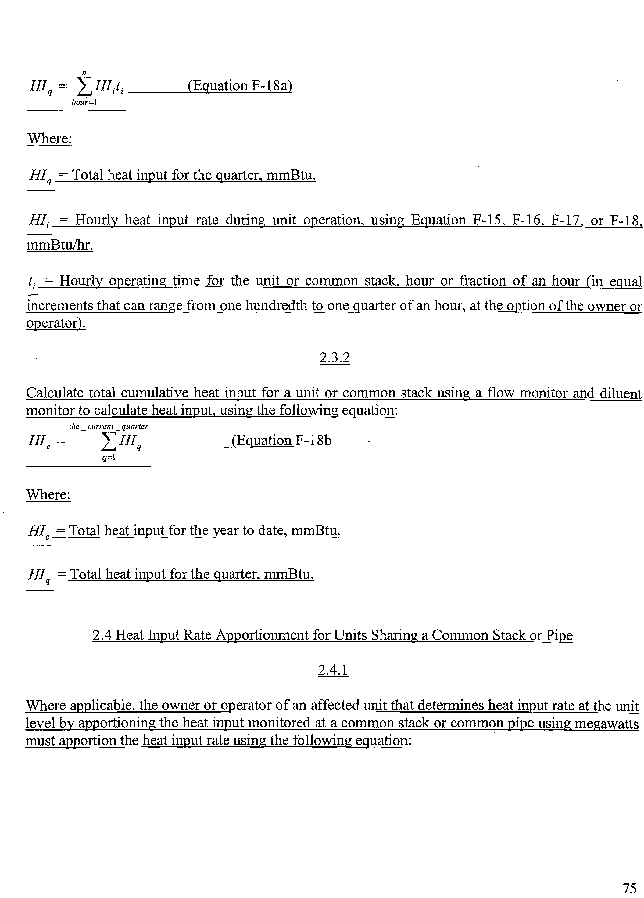
3

---

(FdHY

209

‘V

100

MPV

I

II

II

I

(Equation

A-3a)

A

J

2

O.

9

—%O

2

d).lOO—%H

2

O)

or

MPV

= I

(FH

1

Y

II

100

1

ii

100

I____________________

I

(Equation

A-3b)

A

)%CO

2d

)L100—%H

2

0)

Where:

MPV maximum potential

velocity

(fpm,

standard

wet

basis).

= dry-basis F factor

(dscf7mmBtu)

from Table 1, Section

3.3.5 of

Appenfix

F ,

40

CFR

Part

75.

= carbon-based F

factor

(scf C0

2

/mmBtu)

from Table

1,

Section

3.3.5 of

Appenfix

F

, 40

CFR

Part 75.

Hf = maximum

heat

input (mmBtu!minute)

for

all

units,

combined, exhausting

to the

stack

or

duct

where

the

flow monitor

is

located.

A

inside cross

sectional area

(fl

2)

of the flue

at

the flow monitor location.

°2d

= maximum

oxygen concentration,

percent

dry basis, under normal

operating

conditions.

%CO

2d

= minimum

carbon dioxide

concentration,

percent

dry

basis,

under

normal

operating

conditions.

%H

20

= maximum percent

flue gas moisture

content under

normal

operating

conditions.

2.1.2.2

Span

Values

and Range

Determine

the span

and range of the flow

monitor

as follows.

Convert

the

MPV,

as

determined

in

Section

2.1

.2.1

of this Exhibit, to

the same

measurement

units

of flow rate

that are used

for

dfly

calibration

error tests (e.g., scfh,

kscth, kacfrn,

or differential

pressure(inches

of

water)Nex.

determine

the “calibration

span

value” by

multiplying

the

MPV

(có

étejiT’1ent

dailj

calibration error

units)

by a factor no less

than 1.00

and

no

greater

than 1.25, and

rounding

up

the

result

to

at

least two

significant figures.

For calibration

span values in

inches of water,

retain

at

least

two

decimal

places. Select

appropriate

reference

signals for the

daily calibration

error

tests

as

percentages

of the calibration

span

value,

as

specified

in Section

2.2.2.1 of

this

Exhibit.

Finally

calculate

the “flow rate span

value”

(in

scth)

as

the

product

of the

MPF,

as determined

in

Section

2.1.2.1 of this

Exhibit, times the

same factor

(between

1.00 and

1.25)

that was

used

to

calculate

the

calibration

span value. Round

off the flow rate

span

value

to

the nearest

1000 scth.

Select

the

full

4

---

scale

range

of

the

flow

monitor

so

that

it

is

greater

than

or

equal

to

the

span

value

and

is

consistent

with

Section

2

1

of

this

Exhibit

Include

in

the

morntonng

plan

for

the

unit

calculations

of

the

MPV

MPF,

calibration

span

value,

flow

rate

span

value,

and

full-scale

range

(expressed

both

in

seth

and,

if

different.

in

the

measurement

units

of

calibration).

2.1.2.3

Adjustment

of

Span

and

Range

For

each

affected

unit

or

common

stack,

the

owner

or

operator

must

make

a

periodic

evaluation

of

the

MPV,

span,

and

range

values

for

each

flow

rate

monitor

(at

a

minimum,

an

annual

evaluation

is

required)

and

must

make

any

necessary

span

and

range

adjustments

with

corresponding

monitoring

plan

updates,

as

described

in

paragraphs

(a)

through

(c)

of

this

Section

2.1.2.3.

Span

and

range

adjustments

may

be

required,

for

example,

as

a

result

of

changes

in

the

fuel

supply,

changes

in

the

stack

or

ductwork

configuration,

changes

in

the

manner

of

operation

of

the

unit,

or

installation

or

removal

of

emission

controls.

In

implementing

the

provisions

in

paragraphs

(a)

and

(b)

of

this

Section

2.1.2.3,

note

that

flow

rate

data

recorded

during

short-term,

non-representative

operating

conditions

(e.g..

a

trial

bum

of

a

different

type

of

fuel)

must

be

excluded

from

consideration.

The

owner.

or

operator

must

keep

the

results

of

the

most

recent

span

and.

range

evaluation

on-site,

in

a

format

suitable

for

inspection.

Make

each

required

span

or

range

adjustment

no

later

than

45

days

after

the

end

of

the

quarter

in

which

the

need

to

adjust

the

span

or

range

is

identified.

(a)

If

the

fuel

supply,

stack

or

ductwork

configuration,

operating

parameters,

or

other

conditions

change

such

that

the

maximum

potential

flow

rate

changes

significantly,

adjust

the

span

and

range

to

assure

the

continued

accuracy

of

the

flow

monitor.

A

“significant”

change

in

the

MPV

means

that

the

guidelines

of

Section

2.1

of

this

Exhibit

can

no

longer

be

met,

as

determined

by

either

a

periodic

evaluation

by

the

owner

or

operator

or

from

the

results

of

an

audit

by

the

Agency.

The

owner

or

operator

should

evaluate

whether

any

planned

changes

in

operation

of

theunit

may

affect

the

flow

of

the

unit

or

stack

and

should

plan

any

necessary

span

and

range

changes

needed

to

account

for

these

changes,

so

that

they

are

made

in

as

timely

a

manner

as

practicable

to

coordinate

with

the

operational

changes.

Calculate

the

adjusted

calibration

span

and

flow

rate

span

values

using

the

procedures

in

Section

2.1.2.2

of

this

Exhibit.

(b)

Whenever

the

full-scale

range

is

exceeded

during

a

quarter,

provided

that

the

exceedance

is

not

caused

by

a

monitor

out-of-control

period,

report

200.0

percent

of

the

current

full-scale

range

as

the

hourly

flow

rate

for

each

hour

of

the

full-scale

exceedance.

If

the

range

is

exceeded,

make

appropriate

adjustments

to

the

flow

rate

span,

and

range

to

prevent

future

full-scale

exceedances.

Calculate

the

new

calibration

span

value

by

converting

the

new

flow

rate

span

value

from

units

of

seth

to

units

of

daily

calibration.

A

calibration

error

test

must

be

performed

and

passed

to

validate

data

on

the

new

range.

(c)

Whenever

changes

are

made

to

the

MPV,

full-scale

range,

or

span

value

of

the

flow

monitor,

as

described

in

paragraphs

(a)

and

(b)

of

this

Section,

record

and

report

(as

applicable)

the

new

full

scale

range

setting,

calculations

of

the

flow

rate

span

value,

calibration

span

value,

and

MPV

in

an

updated

monitoring

plan

for

the

unit.

The

monitoring

plan

update

must

be

made

in

the

quarter

in

5

---

which

the

changes become effective. Record and report the adjusted calibration span

and

reference

values

as

parts

of

the records for the

calibration

error test required by

Exhibit

B

to this Appendix.

Whenever

the

calibration span value is

adjusted,

use

reference values for

the

calibration

error

test

that

meet the requirements of

Section 2.2.2.1

of this Exhibit, based on the most recent

adjusted

calibration span value. Perform a

calibration

error test according to Section 2.1 .1 of Exhibit

B to

this

Appendix whenever

making

a

change

to

the flow monitor span or range, unless the

range

change

also triggers a

recertification under Section 1.4

of

this

Appendix.

2.1.3 Mercury Mpnitors

Determine the appropriate span and range

value(s)

for each mercury

pollutant

concentration

monitor,

so that all

expected

mercury concentrations can be determined accurately.

2.1.3.1 Maximum Potential Concentration

The maximum

potential

concentration depends upon the type of coal combusted in

the unit.

For

the

initial MPC

determination, there are three options:

(1)

Use

one of the

following default values:

9 fig/scm for bituminous coal; 10 pjg/scm

for sub-

bituminous coal; 16

iig/scm

for

lignite,

and

1

jig/scm

for waste

coal, i.e., anthracite

cuim

or

bituminous gob. If

different coals are blended, use the highest

MPC for any fuel in the blend;

or

(2)

You may

base

the MPC on the results of site-specific emission

testing using

the

one

of

the

mercury reference

methods in Section 1.6 of this Appendix, if

the

unit

does not

have

add-on

mercury

emission

controls or a flue gas desulfurization system, or if you test upstream

of these

control

devices.

A

minimum

of 3 test runs are required, at the normal operating load. Use the

highest

total

mercury

concentration obtained

in

any

of the tests as the

MPC;

or

(3)

You may

base

the MPC on 720 or more hours of historical CEMS data or data

from

a

sorbent

trap

monitoring

system,

if the

unit does not have add-on mercury

emission controls

or a

flue

gas

desulfurization

system

(or

if the CEMS or sorbent trap system is located upstream

of these

control

devices)

and if

the mercury CEMS or sorbent

trap

system has been tested for relative

accuracy

against one

of the

mercury

reference methods in Section

1.6 of this Appendix and has

met

a relative

accuracy

specification of 20.0%

or

less.

2.1.3.2 Maximum ExpectedConcentration

For units

with FGD

systems that significantly reduce

mercury

emissions

(including

fluidized

bed

units that

use limestone

injection) and for units

equipped

with

add-on mercury emission

controls

(e.g.,

carbon

injection),

determine

the maximum expected mercury

concentration

(MEC)

during

normal,

stable

operation of the unit and emission controls. To calculate the MEC,

substitute

the

MPC

value from

Section

2.1.3.1

of

this Exhibit into Equation

A-2 in Section 2.1.1.2 of

Appendix

A to

40

6

---

CFR

75,

incoorated

by

reference

in

Section

225.140.

For

units

with

add-on

mercury

emission

controls,

base

the

percent

removal

efficiency on

design

engineering

calculations.

For

units

with

FGD

systems,

use

the

best available

estimate

of

the

mercury

removal

efficiency

of

the

FGD

system.

2.1.3.3

Span

and

Range

Value(s)

(a)

For each

mercury

monitor,

determine

a

high

span

value,

by

rounding

the

MPC

value

from

Section

2.1

.3.1

of

this

Exhibit

upward

to

the

next highest

multiple

of

10

jig/scm.

(b)

For

an affected

unit equipped

with

an

FGD

system

or

a

unit

with

add-on

mercury

emission

controls,

if

the

MEC value

from

Section

2.1.3.2

of

this

Exhibit

is

less

than

20

percent

of

the

high

span

value from

paragraph

(a)

of

this

Section,

and

if

the

high

span

value

is

20

jig/scm

or

greater,

define

a

second,

low

span value

of

10

jig/scm.

(c)

If

only

a

high

span

value

is

required,

set

the

full-scale

range

of

the

mercury

analyzer

to

be

greater

than

or

equal

to

the

span

value.

(d)

If

two span values

arecqiiired,

you

may either:

(1)

Use

two separate

(high

and

low)

measurement

scales,

setting

the

range

of

each

scale

to

be

greater

than

or

equal to

the

high or

low

span

value,

as

appropriate

or

(2)

Quality-assure

two segments

of

a

single measurement

scale.

2.1.3.4

Adjustment

of

Span

and Range

For

each affected

unit

or

common

stack,

the

owner

or

operator

must

make

a periodic

evaluation

of

the

MPC,

MEC,

span,

and

range values

for

each

mercury

monitor

(at

a

minimum,

an

annual

evaluation

is

required)

and must

make

any

necessary

span

and

range

adjustments,

with

corresponding

monitoring

plan

updates.

Span

and

range

adjustments

may be

required,

for

example,

as

a

result

of

changes

in the

fuel

supply,

changes

in

the

manner

of

operation

of

the

unit,

or

installation

or

removal

of

emission

controls.

In

implementing

the

provisions

in

paragraphs

(a)

and

(b)

of

this

Section,

data

recorded

during

short-term,

non-representative

process

operating

conditions

(e.g.,

a trial bum

of

a

different

type

of

fuel)

must

be

excluded

from

consideration.

The

owner

or

operator

must keep

the

results

of

the

most

recentpan

and

range

evaluation

on-site,

in

a

format

suitable

for

inspection

Make

each required

span

r

L

110

later

trian

45

days

after

the

end

of

the quarter

in

which

he

ttie

span

or

range

is

identified

except

that

up

to

90

days

after the

end

of

that

quarter

may

be

taken

to

implement

a

span

adjustment

if

the

calibration

gas

concentrations

currently

being

used

for

calibration

error

tests,

system

integrity

checks,

and

lineariti

checks

are

unsuitable

for use

with

the

new

span

value

and

new

calibration

materials

must

be

ordered.

(a)

The

guidelines

of

Section

2.1

of

this

Exhibit

do

not

apply

to

mercury

monitoring

systems.

7

---

(b)

Whenever

a fu11sca1e range

exceedanceoccursduring

a quarter and

is not’caused

by a

monitor

out-of-control

period,

proceed

as follows:

(1) For monitors

with

a single

measurement

scale, report that

the system

was

out of

range

and

invalid

data

was

obtained

until the

readings come back

on-scale

and, if

appropriate,

make

adjustments

to

the

MPC,

span, and range

to

prevent

future

full-scale

exceedances;

or

(2)

For units with two

separate measurement

scales,

if the low range

is exceeded,

no

further

action

is

required, provided

that

the

high.range

is available and

is not out-of-control

or

out-of-service

for

any

reason.

However,

if the high range

is

not able

to provide

quality

assured

data at the time

of

the

low

range exceedance

or

at

any time

during

the continuation

of the

exceedance,

report

that

the

system

was

out-of-control

until the readings

return

to the

low range

or until the high

range is able

to provide

quality

assured

data

(unless

the

reason that the high-scale

range

is

not

able to

provide

quality

assured

data

is because

the

high-scale

range

has been exceeded;

if the

high-scale range

is

exceeded

follow

the procedures in

paragraph

(b)(l)

of this

Section).

(c)

Whenever changes

are

made

to

the

MPC, MEC,

full-scale range,

or span

value of. the

mercury

monitor, record

and report

(as

applicable)

the

new

full-scale

range setting,

the new

MPC

or

MEC

and calculations

of the adjusted

span value

in an updated monitoring

plan.

The

monitoring

plan

update

must

be made

in

the

quarter in which

the

changes

become

effective.

In addition,

record

and

report

the

adjusted

span as

part

of the records

for

the

daily

calibration

error test and

linearity

check

specified

by

Exhibit B

to

this

Appendix.

Whenever

the

span

value is

adjusted,

use

calibration

gas

concentrations

that meet

the

requirements

of Section 5.1

of this Exhibit,

based on

the

adjusted

span

value.

When

a

span

adjustment is

so significant that

the

calibration

gas concentrations

currently

being

used

for

calibration error tests,

system

integrity

checks

and linearity

checks are

unsuitable

for

use with

the new span value,

then

a

diagnostic

linearity or

3-level

system integrity

check

using

the

new

calibration gas concentratiOns

must

be performed

and passed.

Use the

data

validation

procedures

in Section

1

.4(b)(3)

of this Appendix,

beginning

with

the hour in which

the

span

is

changed.

2.2

Design

for

Quality

Control

Testing

2.2.1

Pollutant Concentration

and

CO

2or

02

Monitors

(a)

Design

and

equip

each

pollutant

concentration

and

CO

2 or

02

monitor

with

a

calibration

gas

injection

port that

allows

a check of the entire

measurement

system

when

calibration

gases

are

introduced.

For

extractive

and dilution

type

monitors,

all

ucnitwig

cümponents

exposed

to

the

sample gas, (e.g.,

sample

lines, filters,

scrubbers,

conditioners,

and

as much

of

the

probe as

practicable) are

included

in

the measurement

system.

For in

situ type

monitors,

the

calibration

must

check against

the

injected

gas

for the performance

of all

active electronic and

optical

components

(e.g.

transmitter,

receiver, analyzer).

(b)

Design

and

equip

each

pollutant concentration

or

CO

2

or

02

monitor to

allow

daily

8

---

determinations

of

calibration

error

(positive

or

negative)

at

the

zero-

and

mid-or

high-level

concentrations

specified

in

Section

5.2

of

this

Exhibit.

2.2.2

Flow

Monitors

Design

all

flow

monitors

to

meet

the

applicable

performance

specifications.

2.2.2.1

Calibration

Error

Test

Design

and

equip

each

flow

monitor

to

allow

for

a

daily

calibration

error

test

consisting

of

at

least

two

reference

values:

Zero

to

20

percent

of

span

or

an

equivalent

reference

value

(e.g..

pressure

pulse

or

electronic

signal)

and

50

to

70 percent

of

span.

Flow

monitor

response,

both

before

and

after

any

adjustment,

must

be

capable

of

being

recorded

by

the

data

acquisition

and

handling

system.

Design

each

flow

monitor

to

allow

a

daily

calibration

error

test

of

the

entire

flow

monitoring

system,

from

and

including

the

probe

tip

(or

equivalent)

through

and

including

the

data

acquisition

and

handling

system,

or

the

flow

monitoring

system

from

and

including

the

transducer

through

and

including

the

data acquisition

and

handling system.

2.2.2.2

Interference

Check

(a)

Design

and

equip

each

flow

monitor

with

a

means

to

ensure

that

the

moisture

expected

to

occur

at

the monitoring

location

does

not

interfere

with

the

proper

functioning

of

the

flow

monitoring

system.

Design

and

equip

each

flow

monitor

with

a

means

to

detect,

on

at

least

a

daily

basis,

pluggage

of

each

sample

line and

sensing

port,

and

malfunction

of

each

resistance

temperature

detector

(RTD),

transceiver

or

equivalent.

(b)

Design

and

equip

each

differential

pressure

flow

monitor

to

provide

an automatic,

periodic

back

purging

(simultaneously

on

both

sides

of

the

probe)

or

equivalent

method

of

sufficient

force

and

frequency

to

keep

the

probe

and lines

sufficiently

free

of

obstructions

on

at

least

a

daily

basis

to

prevent

velocity

sensing

interference,

and

a

means

for

detecting

leaks

in

the

system

on

at

least

a

quarterly

basis

(manual

check

is

acceptable).

(c)

Design

and equip

each

thermal

flow

monitor

with

a

means

to

ensure

on

at

least

a

daily

basis

that

the

probe remains

sufficiently

clean

to

prevent

velocity

sensing

interference.

(d)

Design

anu

uip

each

ultrason

‘çw

monitor

with

a

mean.

LO

ensute

ona

least

a

dail

lc

that

the

transceiv.

‘

1

ean

(e.g.,

backn’

:

system

to

prevent

veii

sensinc

interference.

2.2.3

Mercury

Monitors.

Design

and

equip

each

mercury

monitor

to permit

the

introduction

of

known

concentrations

of

elemental

mercury

and

HgCl2

separately,

at

a

point

immediately

preceding

the

sample

extraction

9

---

filtration

system,

suchthat

the

entire

measurement

system

be

checkedlf

the mercury

monitor

does

not

have a

converter,

the

HgCl2

injection

capability

is

not

required.

3. Performance

Specifications

3.1 Calibration

Error

(a)

The

calibration

error

performance

specifications in this

Section

apply only

to

7-day

calibration

error

tests

under

Sections

6.3.1

and

6.3.2

of

this

Exhibit

and

to the

offline

calibration

demonstration

described

in

Section

2.1.1.2

of

Exhibit

B to this

Appendix.

The calibration

error

limits

for

daily

operation

of the

continuous

monitoring

systems

required

under

this

part are

found

in

Section

2.1.4(a)

of Exhibit

B

to

this Appendix.

(b)

The

calibration

error

of

a mercury

concentration

monitor

must

not deviate

from

the

reference

value

of

either

the

zero or

upscale

calibration

gas

by

more

than

5.0

percent

of

the span

value,

as

calculated

using

Equation

A-5 of

this

Exhibit.

Alternatively,

if the

span

value

is 10

ig/scrn,

the

calibration

error

test

results

are also

acceptable

if the absolute

value

of the

difference

between

the

monitor

response

value

and

the

reference

value,

R-A

in Equation

A-5

of this

Exhibit,

is

<=

1.0

LIg/scm.

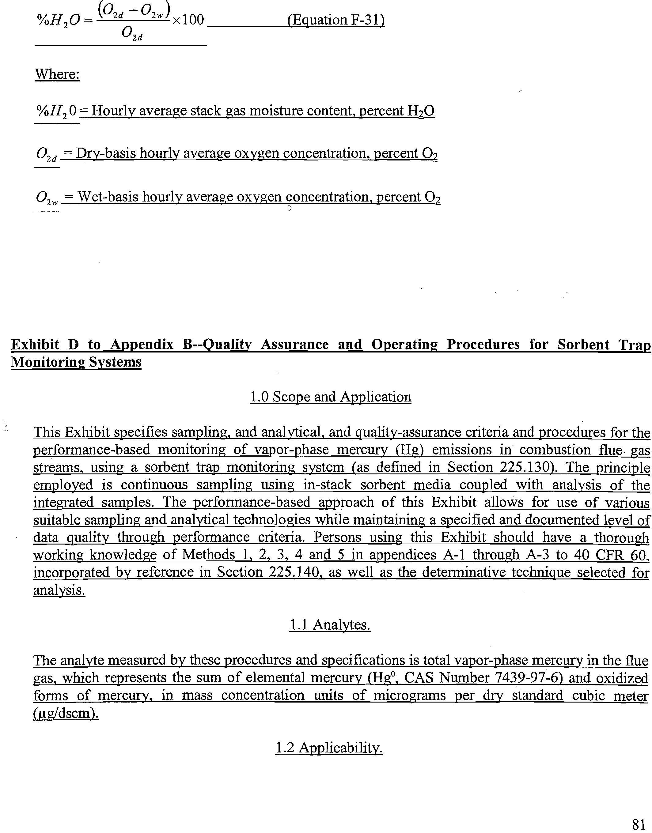
CE

=

x

100

(Equation

A-5)

where,

CE =

Calibration

error

as a percentage

of

the

span

of

the

instrument.

R

=

Reference

value

of

zero

or

upscale

(high-level

or mid-level,

as

applicable)

calibration

gas

introduced

into

the

monitoring

system.

A

Actual

monitoring

system

response

to the

calibration

gas.

S

Span of

the

instrument,

as specified

in

Section

2 of this

Exhibit.

3.2 Linearity

Check

ror

2

CO

olzQ2

monitors

(including

02

:io,;

ased

to measure

CO

2

emissions

or

percent

moisture):

La)

The

error

in linearity

for

each calibration

gas

concentration

(low-,

mid-,

and

high-levels)

must

not

exceed

or

deviate

from the

reference

value

by

more

than

5.0

percent

as

calculated

using

Equation

A-4

of this

Exhibit;

or

10

---

(b)

The

absolute

value

of

the

difference

between

the

average

of

the

monitor

response

values

and

the

average

of

the

reference

values,

R-A

in

Equation

A-4

of

this

Exhibit,

must

be

less

than

or

equal

to

0.5

percent

CO

or

02,

whichever

is

less

restrictive.

(c)

For

the

linearity

check

and

the

3-level

system

integrity

check

of

a

mercury

monitor,

which

are

required,

respectively,

under

Section

1

.4(c)(1

)(B)

and

(c)(

1

)(E)

of

this

Appendix,

the

measurement

error

must

not

exceed

10.0

percent

of

the

reference

value

at

any

of

the

three

gas

levels.

To

calculate

the

measurement

error

at

each

level,

take

the

absolute

value

of

the

difference

between

the

reference

value

and

mean

CEM

response,

divide

the

result

by

the

reference

value,

and

then

multiply

by

100.

Alternatively,

the results

at

any

gas

level

are

acceptable

if

the

absolute

value

of

the

difference

between

the

average

monitor

response

and

the

average

reference

value,

i.e.,

R

—

Aj

in

Equation

A-4

of

this

Exhibit,

does

not

exceed

0.8

Igi’m

3

.

The

principal

and

alternative

performance

specifications

in

this

Section

also

apply

to

the

single-level

system

integrity

check

described

in

Section

2.6

of

Exhibit

B

to

this

Appendix.

LE

R-AI

=

x

100

(Equation

A-4)

where,

LE

=

Percentage

Linearity

error,

based

upon

the

reference

value.

R

=

Reference

value

of

Low-,

mid-,

or

high-level

calibration

gas

introduced

into

the

monitoring

system.

A

=

Average

of

the monitoring

system

responses.

3.3

Relative

Accuracy

3.3.1

Relative

Accuracy

for

CO

2

and

02

Monitors

The relative

accuracy

for

C0

and

0

monitors

must

not

exceed

10.0

percent.

The

relative

accuracy

test

results

are

also

acceptable

if

the

difference

between

-the

mean

value

of

the

C0

or

02 monitor

measurements

and

the

corresponding

reference

method

measurement

mean

value,

calculated

using

equation

A-7

of

this Exhibit,

does

not

exceed

+-

1.0

percent

CO

2

or

02,

d

=

d.

(Equation

A-7’)

where,

11

---

n

= Number

of data

points

d1

=

The difference

between

a referencemethod

value

and

the

corresponding

continuous

emission

monitoring

system

value

(RM—CEM)ata.given..pointintimei

3.3.2

Relative

Accuracy

for Flow

Monitors

(a)

The

relative accuracy

of

flow monitors

must not

exceed

10.0 percent

at any

load

(or

operating)

level

at

which

a

RATA

is

performed

(i.e.,

the low,

mid, or

high

level,

as

defined

in

Section

6.5.2.1

of

this

Exhibit).

(b)

For

affected units

where

the average

of the

flow

reference

method

measurements

of

gas

velocity

at a particular

load

(or

operating)

level

of the

relative

accuracy

test audit

is less

than or

eciual

to

10.0

fp

s, the

difference

between

the mean

value of the

flow

monitor

velocity

measurements

and

the

reference

method

mean

value

in

fps

at that level

must not

exceed

+-

2.0

fps, wherever

the

10.0.

percent

relative accuracy

specification

is

not

achieved.

3.3.3 Relative

Accuracy

for

Moisture

Monitoring

Systems

The

relative accuracy

of

a moisture

monitoring

system

must not

exceed

10.0

percent.

The

relative

accuracy

test

results

are

also acceptable

if the

difference

between

the

mean value

of

the

reference

method measurements

(in percent

H

2

0)

and

the corresponding

mean value

of

the

moisture

monitoring

system

measurements

(in

percent

0),2

H

calculated

using

Equation

A-7

of

this

Exhibit

does

not exceed

+-

1.5

percent

HO.

3.3.4 Relative

Accuracy

for Mercury

Monitoring

Systems

The

relative

accuracy

of

a mercury

concentration

monitoring

system or

a sorbent

trap

monitoring

system must

not

exceed

20.0 percent.

Alternatively,

for affected

units

where

the

average

of the

reference

method

measurements

of mercury

concentration

during

the relative

accuracy

test

audit

is

less than

5.0

jig/scm,

the

test

results

are acceptable

if the difference

between

the

mean

value

of

the

monitor

measurements

and the reference

method

mean value

does

not

exceed

1.0

jig/scm,

in

cases

where

the

relative accuracy

specification

of

20.0 percent

is

not achieved.

3.4 Bias

3.4.1 Flow

Monitors

Flow

monitors

must

not be biased

low

as

determined

by

the

test

procedure

in

Section

7.4

of this

Exhibit.

The bias

specification

applies

to all flow

monitors

including

those

measuring

an

average

gas

velocity

of 10.0

fps

or less.

12

---

3.4.2

Mercury

Monitoring

Systems

Mercury

concentration

monitoring-systems

and

sorbent

trap

monitoring

systems

must

not

be

biased

low

as

determined

by

the

test

procedure

in

Section

7.4

of

this

Exhibit.

3.5

Cycle

Time

The

cycle

time

for

mercury

concentration

monitors,

oxygen

monitors

used

to

determine

percent

moisture,

and

any

other

monitoring

component

of

a continuous

emission

monitoring

system

that

is

required

to

perform

a cycle

time

test

must

not

exceed

15

minutes.

4. Data

Acquisition

and

Handling

Systems

Automated

data

acquisition

and

handling

systems

must

read

and

record

the

full

range

of

pollutant

concentrations

and

volumetric

flow

from

zero

through

span

and

provide

a

continuous,

permanent

record

of

all

measurements

and

required information

as

an

ASCII

flat

file

capable

of

transmission

both

by

direct

computer-to-computer

electronic

transfer

via modem

and

EPA-provided

software

and

by

an

IBM-compatible

personal

computer

diskette.

These

systems

also

must

have

the

capability

of

- interpreting

and

converting

the

individual

output

signals

from

a

flow

monitor,

a

CO,

monitor,

an

02

monitor,

a

moisture

monitoring

system,

a

mercury

concentration

monitoring

system,

and

a

sorbent

trap

monitoring

system,

to

produce

a

continuous

readout

of

pollutant

emission

rates

or

-pollutant

-

mass

emissions

(as

applicable)

in

the

appropriate

units

(e.g.,

lb/hr.

lb/MMBtu, ounces/hr.

tons/br).

These

systems

also

must

have-

-the

capability

of

interpreting

and

converting

the

individual

output

signals

from

a flow

monitor

to produce

a

continuous

readout

of pollutant

mass

emission

rates

in the

units

of the

standard.

Where

CO

2

emissions

are

measured

with

a continuous

emission

monitoring

system,

the

data

acquisition

and

handling

system

must

also

produce a readout

of

CO

2

mass

emissions

in tons.

Data

acquisition and

handling

systems

must

also

compute

and

record

monitor

calibration

error;

any

bias

adjustments

to

mercury

pollutant

concentration

data,

flow

rate

data,

or

mercury

emission

rate

data.

5. Calibration

Gas

5.1

Reference

Gases

-

-

-

For

the

purposes

of

this

Appendix,

calibration

gases

include

the

following:

5.1.1

Standard

Reference

Materials

(SRM)

These

calibration

gases

may

be

obtained

from

the

National

Institute

of

Standards

and

Technology

(NIST)

at the

following

address:

Quince

Orchard

and

Cloppers

Road,

Gaithersburg,

MD

20899-

13

---

0001

5.1.2

SRM-Eguivalent

Compressed

Gas

Primary

Reference

Material

(PRM)

Contact

the

Gas

Metrology

Team,

Analytical

Chemistry

Division,

Chemical

Science

and

Technology

Laboratory

of

NIST,.at

the

address

in.

Section

5.l.l,for

a list

of

vendors

and

cylinder

gases.

5.1.3

NIST

Traceable

Reference Materials

Contact

the

Gas

Metrology

Team,

Analytical

Chemistry

Division,

Chemical

Science

and

Technology

Laboratory

of

NIST,

at the

address

in

Section

5.1.1,

for

a list

of

vendors

and

cylinder

gases

that

meet

the

definition

for a

NIST

Traceable

Reference

Material

(NTRM)

provided

in

40

CFR

72.2,

incorporated

by

reference

in Section

225.140.

5.1.4

EPA

Protocol

Gases

(a)

An

EPA

Protocol

Gas

is

a

calibration

gas mixture

prepared

and

analyzed

according

to

Section

2

of

the

“EPA

Traceability

Protocol

for Assay

and

Certification

of

Gaseous

Calibration

Standards,”

September

1997,

EPA-600/R-97/121

or

such

revised

procedure

as approved

by

the

Administrator

(EPA

Traceability

Protocol).

(b)

An EPA

Protocol

Gas

must

have

a

specialty

gas

producer-certified

uncertainty

(95-percent

confidence

interval)

that

must

not

be

greater

than

2.0 percent

of the

certified

concentration

(tag

value)

of the

gas

mixture.

The

uncertainty

must

be

calculated

using

the

statistical

procedures

(or

equivalent statistical

techniques)

that

are

listed

in Section

2.1.8

of the

EPA

Traceability

Protocol.

(c)

A

copy

of EPA-600/R-97/121

is

available

from

the

National

Technical

Information

Service,

5285

Port

Royal

Road,

Springfield.

VA,

703-605-6585

or

http://www.ntis.gov,

and

from

http://www.epa.

gov/ttnlemc/news.html or

http://

www.epa.gov/appcdwww/tsb/index.html.

5.1.5

Research

Gas

Mixtures

Research gas

mixtures

must

be

vendor-certified

to

be

within

2.0

percent

of

the

concentration

specified

on

the cylinder

label

(tag

value),

using

the

uncertainty

calculation

procedure

in

Section

2.1.8

of the

“EPA

Traceability

Protocol

for

Assay

and

Certification

of

Gaseous

Calibration

Standards,” September

1997,

EPA-600/R-97/121.

Inquiries

about

the

RGM

program

should

be

directed to: National

Institute

of

Standards

and

Technology,

Analytical

Chemistry

Division,

Chemical Science

and

Technology Laboratory,

B-324

Chemistry,

Gaithersburg,

MD

20899.

5.1.6

Zero

Air

Material

14

---

Zéroafr-rnaterialis

ipóratedb/refeTence

iii

Sëctioft225.T40.

5.1.7

N1ST/EPA-Approved

Certified

Reference

Materials

Existing

certified

reference

materials

(CRMs) that

are

still

within

their

certification

period

may

be

used

as

calibration

gas.

5.1.8

Gas Manufacturer’s

Intermediate

Standards

Gas

manufacturer’s

intermediate

standards

is

defined

in

40

CFR 72.2,

incorporated

by

reference

in

Section

225.140.

5.1.9

Mercury

Standards

For

7-day

calibration

error

tests

of

mercury

concentration

monitors

and

for

daily

calibration

error

tests

of

mercury

monitors,

either

NIST-traceable

elemental

mercury

standards

(as

defined

in

Section

225.130)

or

a

NIST-traceable

source

of

oxidized

mercury

(as

defined

in

Section

225.130)

may

be

used.

For linearity

checks,

NIST-traceable

elemental

mercury

standards

must

be

used.

For

3-

level

and single-point

system

integrity

checks

under

Section

1

.4(c)(1)(E)

of

this

Appendix,

Sections

6.2(g)

and 6.3.1

of

this Exhibit,

and

Sections

2.1.1,

2.2.1

and

2.6

of

Exhibit

B

to

this

Appendix,

a

NIST

traceable

source

of

oxidized

mercury

must

be

used.

Alternatively,

other

NIST-traceable

standards

may be

used-for

the

required

checks,

subject

to

the

approval

of

the

Agency.

Notwithstanding

these

requirements,

mercury

calibration

standards

that

are

not

NIST-traceable

may

be

used

for

the

tests

described

in

this

Section

until

December

31, 2009.

However,

on

and

after

January

1,

2010,

only

NIST-traceable

calibration

standards

must

be

used

for

these

tests.

5.2

Concentrations

Four

concentration

levels

are

required

as

follows.

5.2.1

Zero-level

Concentration

0.0

to

20.0

percent

of

span,

including

span

for

high-scale

or

both

low-

and

high-scale

for

CO,

and

02

monitors,

as

appropriate.

5.2.2

Low-level

Concentration

20.0 to

30.0 percent

of

span, including

span

for

high-scale

or

both-low--

and high-scale

for

CQ

2

and

Q

monitors,

as

appropriate.

5.2.3

Mid-level

Concentration

50.0 to

60.0

percent

of

span,

including span

for

high-scale

or

both

low-

and

high-scale

for

CO

2

and

15

---

Q2

monitors,:

asappropri’ate

5.2.4High-level

Concentration

80.0 to

100.0

percent

of span,

including

span

for

high-scale

orboth

low-and

high-scale

for

CO

2

and

Q2

monitors,

as

appropriate.

6.

Certification

Tests

and

Procedures

6.1 General

Requirements

6.1.1

Pretest

Preparation

Install

the

components

of the

continuous

emission

monitoring

system

(i.e.,

pollutant

concentration

monitors,

CO,

or

02

monitor,

and

flow

monitor)

as specified

in Sections

1, 2, and

3

of

this

Exhibit,

and

prepare

each

system

component

and

the combined

system

for

operation

in

accordance

with

the

manufacturer’s

written

instructions.

Operate

the

unit(s)

during

each

period

when

measurements

are

made.

Units

may

be tested

on

non-consecutive days.

To

the extent

practicable,

test

the

DABS

software

prior

to

testing

the

monitoring

hardware.

6.1.2

Requirements

for

Air

Emission

Testing

Bodies

(a)

On and

after

January

1, 2009,

any

Air Emission

Testing

Body

(AETB)

conducting

relative

accuracy

test

audits

of

CEMS

and

sorbent

trap

monitoring

systems

under

Part

225,

Subpart

B,

must

conform

to the

requirements

of

ASTM

D7036-04

(incorporated

by

reference

under

Section

225.140).

This

Section

is

not

applicable

to

daily

operation,

daily

calibration

error

checks,

daily

flow

interference

checks,

quarterly

linearity

checks

or

routine

maintenance

of CEMS.

(b’)

The AETB

must

provide

to

the affected

source(s)

certification

that the

AETB

operates

in

conformance

with,

and

that

data

submitted

to the

Agency

has

been

collected

in accordance

with,

the

requirements

of

ASTM

D7036-04

(incorporated

by

reference

under

Section:225.i4O).

This

certification

may

be

provided

in

the

form

of:

(1)

A

certificate

of

accreditation

of relevant

scope

issued

by

a recognized,

national

accreditation

body:

or

(2)

A

letter

of

certification

signed

by

a

member

of

the senior

management

staff

of the AETB.

(c)

The AETB

must

either

provide

a

Qualified

Individual

on-site

to

conduct

or

must

oversee

all

relative

accuracy

testing

carried

out

by

the AETB

as

required

in ASTM

D7036-04

(incorporated

by

reference

under

Section

225.140).

The

Qualified

Individual

must provide

the affected

source(s)

with

copies

of the

qualification credentials

relevant

to the

scope

of the

testing

conducted.

16

---

6.2

Li±

Check

the

linearity

of

each

CO,.

Hg,

and

02

monitor

while

the

unit,

or

group

of

units

for

a

common

stack,

is

combustingfuel.

atconditions

of

typical

stack

temperature

and

pressure;

it

is

not

necessary

for

the

unit

to

be

generating

electricity

during

this

test.

For

units

with

two

measurement

ranges

(high

and

low)

for

a

particular

parameter,

perform

a

linearity check

on

both

the

low

scale

and

the

high

scale.

For

on-going

quality

assurance

of

the

CEMS,

perform

linearity

checks,

using

the

procedures

in

this

Section,

on

the

range(s)

and

at

the

frequency

specified in

Section

2.2.1

of

Exhibit

B

to

this

Appendix.

Challenge

each

monitor

with

calibration

gas,

as

defined

in

Section

5.1

of

this

Exhibit,

at

the

lowmid-,

and high-range

concentrations

specified

in

Section

5.2

of

this

Exhibit.

Introduce

the

calibration

gas

at

the gas

injection

port,

as

specified

in

Section

2.2.1

of

this Exhibit.

Operate

each

monitor

at

its

normal

operating

temperature

and

conditions.

For

extractive

and

dilution

type

monitors,

pass

the calibration

gas

through

all

filters,

scrubbers,

conditioners,

and

other

monitor

components

used

during

normal

sampling

and

through

as

much

of

the

sampling

probe

as

is

practical.

For

in-situ

type

monitors,

perform

calibration

checking

all

active

electronic

and

optical

components..

including

the

transmitter,

receiver,

and

analyzer.

Challenge

the

monitor

three

times

with

each

reference

gas

(see

example

data

sheet

in

Figure

1).

Do

not

use

the

same

gas

twice

in

succession.

To

the

extent

practicable,

the

duration

of

each

linearity

test,

from

the

hour

of

the

first

injection

to

the

hour

of

the last

injection,

must

not

exceed

24

unit

operating

hours.

Record

the

monitor

response

from

the

data acquisition

and

handling

system.

For

each

concentration,

use

the

average

of

the

responses

to

determine

the

error

in

linearity

using Equation

A-4

in

this

Exhibit.

Linearity

checks

are

acceptable

for

monitor

or

monitoring

system

certification,

recertification,

or

quality

assurance

if

none

of

the

test

results

exceed

the

applicable

perfonnance

specifications

in

Section

3.2

of

this

Exhibit

The

status

of

emission

data

from

a

CEMS

prior

to

and

during

a

linearity

test

period

must

be

determined

as

follows:

(a)

For

the initial

certification

of

a

CEMS,

data

from the

monitoring

system

are

considered

invalid

until

all certification

tests,

including

the

linearity

test,

have

been

successfully

completed,

unless

the

conditional

data validation

procedures

in

Section

1

.4(b)(3) of

this

Appendix

are

used.

When

the

procedures

in

Section

1

.4(b)(3)

of

this

Appendix

are

followed,

the

words

“initial

certification”

apply

instead

of

“recertification,”

and

complete

all

of

the

initial

certification

tests

by

January

1,

2009,

rather

than

within

the

time

periods

specified

in

Section

1

.4(b)(3)(D)

of

this

Appendix

for

the

individual

tests.

(b)

For

tue

ruuL

assurance

linearity

checks

required

by

Section

2.2.1

of

Exhibit

B

to

this

Appendix,

use

the

data validation

proc:

cection

2.2.3

of

Exhibit

B

to

this

Appendix.

(c)

When

a

linearity

test

is

required

as

a

diagnostic

test

or

for

recertification,

use

the

data

validation

procedures

in

Section

1.4

(b)(3)

of

this

Appendix.

(d)

For linearity

tests of

non-redundant

backup

monitoring

systems,

use

the

data

validation

procedures

in

Section

1

.4(d)(2)(C)

of

this

Appendix.

17

---

(e)

theexpiratiorrofagraceperkod

use

the

data

validation

procedures

in Sections 2.2.3

and 2.2.4,

respectively, of

Exhibit

B

to this

Appendix.

(f)

For all other

linearity

checks, use

the data validation

procedures

in Section 2.2.3

of Exhibit

B to

this Appendix.

(g)

For

mercury monitors,

follow the

guidelines in Section

2.2.3 of

this

Exhibit

in

addition

to

the

applicable

procedures

in Section 6.2 when

performing

the system

integrity

checks

described

in

Section

1.4(c)(1)(E)

and in

Sections 2.1.1,

2.2.1, and 2.6

of Exhibit B to this

Appendix.

(h)

For

mercury concentration

monitors,

if moisture

is added to the

calibration

gas

during

the

recuired

linearity

checks

or system integrity

checks,

the

moisture content

of the calibration

gas

must

be accounted

for. Under these

circumstances,

the dry basis

concentration

of the calibration

gas

must

be

used to

calculate the linearity

error

or measurement

error

(as applicable).

6.3 7-Day

Calibration

Error

Test

6.3.1 Gas

Monitor 7-day Calibration

Error Test

Measure the

calibration error of each

mercury

concentration monitor,

and

each

CO

2 or

0,

monitor

while the

unit is combusting

fuel

(but

not

necessarily

generating

electricity)

once each

day

for

7

consecutive

operating

days

according to the

following procedures.

For mercury

monitors,

you

may

perform this test using

either elemental mercury

standards

or a NIST-traceable

source

of

oxidized

mercury.

Also

for

mercury

monitors, if

moisture is

added to the calibration

gas,

the added

moisture

must be

accounted for

and the

dry-basis

concentration

of the calibration

gas

must

be

.used

to

calculate

the

calibration

error.

(In

the

event

that unit

outages occur

after the

commencement

of

the

test,

the

7

consecutive

unit

operating

days need

not

be 7 consecutive calendar

days.)

Units

using

dual

span monitors

must

perform

the

calibration error

test

on both high-

and low-scales

of

the

pollutant

concentration

monitor.

The calibration

error test

procedures

in

this

Section and

in

Section

6.3.2

of

this

Exhibit

must also be used

to perform the

daily assessments and

additional

calibration

error

tests

required

under

Sections 2.1.1

and

2.1.3

of Exhibit

B

to

this

Appendix. Do not

make

manual

or

automatic

adjustments to the monitor

settings

until after taking measurements

at both

zero

and

high

concentration

levels

for that

day during the

7-day

test. If automatic

adjustments

are

made

following

both

injections,

conduct the

calibration error

test such

that

the magnitude of

the

adjustments

can

be

determined and

recorded.

Record and

report test results

for cach

day

using

the

unadjusted

concentration

measured

in

the calibration

error

test prior to making

any manual

or

automatic

adjustments

(i.e.,

resetting the

calibration). The calibration

error

tests should

be approximately

24

hours

apart,

(unless

the

7-

day

test

is performed

over

non-consecutive

days).

Perform

calibration

error tests at

both the zero-level

concentration

and high-level

concentration,

as specified

in

Section

5.2

of this

Exhibit. Alternatively,

a

mid-level

concentration

gas

(50.0

to

60.0

percent

of

the

span

value)

may be used

in

lieu of the high-level

gas,

provided

that

the mid-level

gas

is

more

representative

of the actual

stack gas concentrations.

Use only

calibration

gas, as specified

in

Section

18

---

5.1

of

this

Ehib’iL

Jñtroducethe’

calibration

gas

at

the’gasiniection

port,’

as

specffiediriSecón22J

of

this

Exhibit.

Operate

each

monitor

in

its

normal

sampling

mode.

For

extractive

and

dilution

type

monitors,

pass

the

calibration

gas

through

all

filters,

scrubbërs,

conditioners,

and•

other

monitor

components

used

during

normal

sampling

and

through

as:much.

of

the

sampling

probe

as

is

practical.

For

in-situ

type

monitors,

perform

calibration,

checking

all

active

electronic

and

optical

components,

including

the transmitter,

receiver,

and

analyzer.

Challenge

thern

pollutant

concentration

monitors

and

cQ

or

02

monitors

once

with

each

calibration

gas. Record

the

monitor

response

from

the

data

acquisition

and handling

system.

Using

Equation

A-5

of

this

Exhibit,

determine

the

calibration

error

at

each

concentration

once

each

day

(at

approximately

24-hour

intervals)

for

7

consecutive

days

according

to

the procedures

given

in

this

Section.

The

results

of

a

7-day

calibration

error

test

are

acceptable

for monitor

or

monitoring

system

certification,

recertification

or

diagnostic

testing

if

none

of

these

daily

calibration

error

test

results

exceed

the

applicable

performance

specifications

in

Section

3.1

of

this Exhibit.

The

status

of

emission

data

from

a

gas

monitor

prior

to

and

during

a

7-

day

calibration

error

test

period

must

be

determined

as

follows:

(a)

For

initial

certification,

data

from

the

monitor

are

considered

invalid

until

all

certification

tests.

including

the

7-day

calibration

error

test,

have

been

successfully

completed,

unless

the

conditional

data

validation

procedures

in

Section

1

.4(b)(3)

of

this

Appendix

are

used.

When

the

procedures

in

Section

1.4(b)(3)

of

this

Appendix

are

followed,

the

words

“initial

certification”

apply

instead

of

“recertification,”

and complete

all

of

the

initial

certification

tests

by

January

1,

2009,

rather

than

within

the

time

periods

specified

in

Section

1

.4(b)(3)(D)

of

this

Appendix

for

the

individual

tests.

(b)

When

a

7-day

calibration

error

test

is

required

as

a

diagnostic

test

or

for

recertification,

use

the

data validation

procedures

in

Section

1

.4(b)(3)

of

this

Appendix.

6.3.2

Flow

Monitor

7-day

Calibration

Error

Test

Flow

monitnr

installed

on

peaking

units

(as

defined

in

40

CFR

72.2,

incorporated

by

reference

in

Section

225

140)

are

excivpteu

1Iou

‘

1

ay

calibration

error

test

requirements

of

this

part

In

all

other

cases,

perform

the

7-day

calibration

erir

test

of

a

flow

monitor,

when

required

for

certification,

recertification

or

diagnostic

testing,

according

io

:e

foHowing

procedures.

Introduce

the reference

signal

corresponding

to

the

values

specified

in

Section

2.2.2.1

of

this

Exhibit

to

the

probe

tip

(or

equivalent),

or

to

the

transducer.

During

the

7-day

certification

test

period,

conduct

the

calibration

error

test

while

the

unit

is

operating

once

each

unit

operating

day

(as

close

to

24-hour

intervals

as

practicable).

In

the

event

that

unit outages

occur

after

the

commencement

of

the

test,

the

7

consecutive

operating

days

need

not

be 7

consecutive

calendar

days.

Record

the

flow

monitor

responses

by

means

of

the

data

acquisition

and

handling

system.

Calculate

the

calibration

error

using

Equation

A-6

of

this Exhibit.

Do

not

perform

any

corrective

maintenance,

repair,

or

replacement

upon

the

flow

monitor

during

the

7-day

test

period

other

than

that

required

in

the

quality

assurance/quality

control

plan

required

by

Exhibit

B

to

this

Appendix.

Do

not

make

adjustments

between

the

zero

and

high

reference

level

measurements

on

any

day

during

the

7-day

test.

If

the

flow

monitor

operates

within

the

calibration

error

performance

specification

(i.e.,

less

than

or

equal

to

3.0

percent

error

each

day

and

requiring

no

corrective

maintenance,

repair,

or

replacement

during

the

7-

19

---

day

testperiod),

alLmaintenance•aetivjtiés

and

the magnitude

of any

adjustments.

Record

output

readings

from the

data

acquisition

and

handling

system

bef6re

and

after

all

adjustments.

Record

and

report

all

calibration

error test

results

using

the

unadjusted

flow

rate

measured

in the calibration

error test

prior

to resetting

the

calibration.

Record

all adjustments

made

during

the

7-day period

at the time

the

adjustment

is made,

and

report

them

in the certification

or recertification

ap.plication

The. status

of emissions

data

from

a flow

monitor

prior

to and

during

a 7-day

calibration

error test

period

must be

determined

as

follows:

(a)

For

initial

certification,

data

from

the

monitor

are considered

invalid

until

all

certification

tests,

including

the

7-day

calibration

error test,

have been

successfully

completed,

unless

the

conditional

data

validation

procedures

in

Section

l.4(b)(3)

ofthis

Appendix

are

used.

When

the

procedures

in

Section

1

.4(b)(3)

of

this Appendix

are followed,

the

words

?initial

certification’

apply

instead

of

“recertification,”

and

complete

all of the

initial

certification

tests

by

January 1,

2009,

rather

than

within the

time

periods

specified

in Section

1

.4(b)(3)(D)

of

this Appendix

for

the

individual

tests.

(b) When

a 7-day

calibration

error

test is

required as

a diagnostic

test or

for

recertification,

use the

data validation

procedures

in Section

1

.4(b)(3).

CE

=

x

100

(Equation

A-6)

S

where:

CE

= Calibration

error

as a

percentage

of span.

R =

Low or

high level

reference

value

specified

in

Section

2.2.2.1

of

this Exhibit.

A = Actual

flow

monitor

response

to

the reference

value.

S

= Flow

monitor

calibration

span

value

as

determined

under

Section

2.1.2.2 of this

Exhibit.

6.3.3

For

gas

or

flow

monitors

installed

on peaking

units,

the

exemption

from performing

the

7-day

calibration

error test

applies

as long as

the unit continues

to meet the

definition

of

a

peaking

unit

in

40

CFR

72.2, incorporated

by

reference

in

Section

225.140.

However,

if at

the end

of a

particular

calendar

year

or ozone season,

it is

determined

that

peaking

unit

status has

been lost,

the

owner

or

operator

must

perform

a diagnostic

7-day calibration

error test

of each monitor

installed

on

the

unit,

by

no

later

than December

31 of

the

following

calendar

year.

6.4 Cycle

Time

Test

20

---

Perform

cycle

time

tests

for

each

pollutant

concentration

monitor

and

continuous

emission

monitoring

system

while

the

unit

is

operating,

according

to

the

following

procedures.

Use

a zero-

level

and

a

high-level

calibration

gas’

(asdefined.

in.

Section

5.2

of

this

Exhibit)

alternately.

For

mercury

monitors,

the

calibration

gas

used

for

this

test

may

either

be

the elemental

or

oxidized

form

of mercury.

To

determine

the

downscale

cycle

time,

measure

the

concentration

of

the

flue

gas

emissions

until

the

response

stabilizes.

Record

the

stable

emissions

value.

Inject

a

zero-level

concentration

calibration

gas

into

the

probe

tip

(or

injection

port

leading

to

the

calibration

cell,

for

in

situ

systems

with

no

probe).

Record

the

time

of

the

zero

gas

injection,

using

the

data

acquisition

and

handling

system

(DAHS).

Next,

allow

the monitor

to

measure

the

concentration

of the

zero

gas

until

the

response

stabilizes.

Record

the

stable

ending

calibration’

gas

reading.

Determine

the

downscale

cycle

time

as the

time

it

takes

for

95.0

percent

of the

step

change

to

be

achieved

between

the

stable

stack

emissions

value

and

the

stable

ending

zero

gas

reading.

Then

repeat

the

procedure,

starting

with

stable stack

emissions

and

injecting

the

high-level

gas,

to

determine

the

upscale

cycle

time.

which

is

the

time

it

takes

for

95.0

percent

of

the

step

change

to

be

achieved

between

the

stable

stack

emissions

value

and

the

stable

ending

high-level

gas

reading.

Use the

following

criteria

to

assess

when

a

stable

reading

of

stack

emissions

or

calibration

gas

concentration

has

been

attained.

A

stable

value

is equivalent

to

a reading

with

a

change

of

less

than

2.0

percent

of

the

span

value’

for

2

minutes,

or

a

reading

with

a change

of

less

than

6.0

percent

from

the

measured

average

concentration

over

6 minutes.

Alternatively,

the

reading

is considered

stable

if it

changes

by

no

more

than

0.5

ppm,

0.5

g/m

3

(for

mercury) for

two

minutes.

(Owners

or

operators

of systems

which

do

not

record

data

in

1-minute

or

3-minute

intervals

may.

petition

the

Agency

for

alternative

stabilization

criteria). For

monitors

or

monitoring

systems that

perform

a

series

of

operations

(such

as purge, sample,

and

analyze),

time

.the injections

of

the

calibration

gases

so

they

will

produce

the

longest

possible

cycle

time.

Refer

to

Figures

6a

and

6b

in

this

Exhibit

for

example

calculations

of

upscale

and

downscale

cycle

times.

Report

the

slower

of

the

two

cycle

times

(upscale

or

downscale)

as

the

cycle

time

for

the

analyzer.

On

and

after

January

1,

2009,

record

the

cycle

time

for

each

component

analyzer

separately.

For

time-shared

systems,

perform

the

cycle

time

tests

at

each

probe

locations

that

will

be

polled

within

the

same

15-minute

period

during

monitoring

system

operations.

To

determine

the

cycle

time

for

time-shared

systems,

at

each

monitoring

location,

report

the

sum

of

the

cycle

time

observed

at that

monitoring

location

plus

the

sum

of

the

time

required

for

all

purge

cycles

(as

determined

by the

continuous

emission

monitoring

system

manufacturer)

at

each

of

the

probe

locations

of

the

time-shared

systems.

For

monitors

with

dual

ranges,

report

the

test

results

for

each

range

separately.

Cycle

time

test

results

are

acceptable

for

monitor

or

monitoring

system

certification,

recertification

or

diagnostic

testing

if

none

of

the

cycle

times

exceed

15

minutes.

The

status

of

emissions

data

from

a

monitor

prior

to

and

during

a

cycle

time

test

period

must

be

determined

as

follows:

(a)

For

initial

certification,

data

from

the

monitor

are

considered

invalid

until

all

certification

tests,

including

the

cycle

time

test,

have

been

successfully

completed,

unless

the

conditional

data

validation procedures

in Section

1

.4(b)(3) of

this

Appendix

are

used.

When

the

procedures

in

Section

1 .4(b)(3) of this

Appendix

are

followed,

the

words

“initial

.certification”

apply

instead

of

“recertification,”

and

complete

all of

the

initial

certification

tests

by

January

1,

2009,

rather

than

21

---

within’the’tinie

periods’speci’ffedin Section

.4(b4E•3)(DYofthisAppendix’fortheindividüai.

tests.

(b)

When a cycle time test is required as a diagnostic test or

for rcertificatiön,

use the

data

validation

procedures in Section

1

.4(b)(3.)

of this Appendix.

6.5 Relative Accuracy and

Bias Tests

(General Procedures)

Perform

the required relative accuracy test

audits

(RATAs)

as follows for each flow

monitor,

each

Q2

or CO

2 diluent monitor used to calculate heat input, each

mercury concentration

monitoring

system, each sorbent

trap

monitoring system,

and each moisture monitoring system:

(a) Except as

otherwise provided

in

this paragraph,

perform

each RATA while the

unit

(or

units,

if

more than one unit exhausts into the flue) is combusting the fuel that

is a normal primary

or

backup

fuel for that unit

(for

some

units, more than one type

of fuel may be considered normal,

e.g.,

a

unit

that combusts

gas or oil on

a seasonal

basis).

For units that co-fire fuels

as

the

predominant

mode

of

operation, perform the RATAs while co-firing. For mercury

monitoring

systems,

perform the

RATAs while the unit is combusting coal. When relative accuracy test audits are

performed

on

CEMS

installed on

bypass

stacks/ducts,

use

the

fuel

normally combusted

by

the

unit (or

units,

if

more

than one unit exhausts into the

flue)

when emissions

exhaust through the bypass

stack/ducts.

(b)

Perform each RATA at the load

(or

operating)

level(s)

specified

in Section 6.5.1 or

6.5.2

of this

Exhibit or in Section 2.3.1.3 of Exhibit B to this Appendix, as applicable.

(c)

For monitoring

systems with

dual ranges,

perform

the relative

accuracy

test on

the

range

normally used

for measuring emissions. For

units with add-on mercury

controls

that

operate

continuously

rather than

seasonally,

or for units

that

need a dual, range to record high

concentration

“spikes”