BEFORE THE ILLINOIS POLLUTION CONTROL BOARD

IN THE MATTER OF:

WATER QUALITY STANDARDS AND

EFFLUENT LIMITATIONS FOR THE

CHICAGO AREA WATERWAY SYSTEM

AND THE LOWER DES PLAINES RIVER:

PROPOSED AMENDMENTS TO 35 Ill.

Adm. Code Parts 301, 302, 303 and 304

R08-9

(Rulemaking

-

Water)

PRE-FILED TESTIMONY OF SCUDDER D. MACKEY

Introduction

My name is Scudder D. Mackey and I am an Environmental Consultant specializing in

aquatic habitat mapping and characterization in both riverine and lake systems. I am the owner

of Habitat Solutions NA, which is an independent environmental consulting firm. I currently

hold dual appointments as a Visiting Research Professor in the Departments of Biological

Sciences and Geological Sciences at the University of Windsor, Ontario, Canada. I hold a

Bachelor of Science Degree in the Geological Sciences from Hobart College and a Master of

Science in Geology from the University of Wisconsin - Madison. I received a Doctor of

Philosophy Degree in Geology (fluvial sedimentology) from the State University of New York at

Binghamton.

My areas of technical specialization are in aquatic habitat characterization and mapping;

developing biophysical linkages to habitat; surface and watershed hydrology; nearshore, coastal,

and riverine processes; and application of geospatial data and analyses (GIS) to Great Lakes

aquatic ecosystems. I served as Supervisor for the Lake Erie Geology Group for the Ohio

Department of Natural Resources and worked for the Great Lakes Governors as Project

Implementation Manager with the Great Lakes Protection Fund (GLPF). I currently serve as a

member of Lake Erie Habitat Task Group for the Great Lakes Fisheries Commission and the AIS

I

---

Barrier Advisory Panel and Rapid Response Team for the USACE Chicago Waterway electric

field barrier project.

In 1995, I received the Outstanding Paper Award for the Journal of Sedimentary

Research. In 2001, I received letters of commendation from the Ohio Senate and the U.S. House

of Representatives for services to the People of the State of Ohio and the Natural Resources of

Lake Erie. In 2005, 1 was retained by the Water Quality Board of the International Joint

Commission to fully explore the role of physical integrity as part of a comprehensive ongoing

review of the Great Lakes Water Quality Agreement. Also in 2005, I was the co-editor of a

Special Issue of the Journal of Great Lakes Research entitled

Nearshore and Coastal Habitats of

the Laurentian Great Lakes,

a collection of 14 peer-reviewed papers focused on the physical,

chemical, and biological characteristics of Great Lakes nearshore and coastal habitats. In 2006, I

was a co-investigator on a USFWS Great Lakes Fisheries Restoration Act funded project to

create a framework and develop a process to systematically identify, coordinate, and implement

aquatic and fish habitat restoration opportunities in the Lake Huron to Lake Erie Corridor (St.

Clair River, Lake St. Clair, Detroit River). This project considered potential restoration

opportunities within a context of long-term effects of global climate change.

Current ongoing projects include: Identification and mapping of potential lake trout

spawning habitat in the Eastern Basin of Lake Erie in cooperation with the Ontario Ministry of

Natural Resources and the New York Department of Environmental Conservation; river mouth

mapping and instream aquatic habitat assessments for three urban rivers in the Toronto area in

cooperation with the Toronto Regional Conservation Authority; riverine fish habitat assessments

in the Sandusky River and Sandusky Bay areas in cooperation with Ohio State University and

2

---

Ohio Department of Natural Resources; and removal of the Ballville Dam on the Sandusky River

in cooperation with the Ohio Department of Natural Resources.

Review of my resume (Attachment 1) will reveal that my work has been focused on

developing linkages between physical processes, physical habitat, and the organisms that use

those habitats.

My work is based on first principles and considers habitat function, pattern, and

connectivity; and includes the use of remote sensing technologies (sidescan sonar) in addition to

more traditional habitat assessment techniques. This experience brings a unique perspective to

the Chicago Area Waterway System.

Overview

The testimony presented here today will be focused primarily on the aspects of

physical

habitat

related to the Aquatic Life Use designations proposed in IPCB rulemaking R08-9 and the

methodology that IEPA used to designate those Aquatic Life Uses. My testimony has three

components: 1) I will demonstrate that the data and methodology used by IEPA is inaccurate,

flawed, and does not adequately consider all of the key elements necessary to assess the

condition of aquatic habitats, 2) 1 will show that it is unlikely that the current proposed standards

will significantly improve fish community structure and diversity in the Chicago Area Waterway

System, and 3) I will suggest an alternative strategy that integrates all of the fundamental habitat

characteristics necessary to maximize the productive and ecological capacity of the waterway, a

strategy that the Metropolitan Water Reclamation District of Greater Chicago is currently

pursuing.

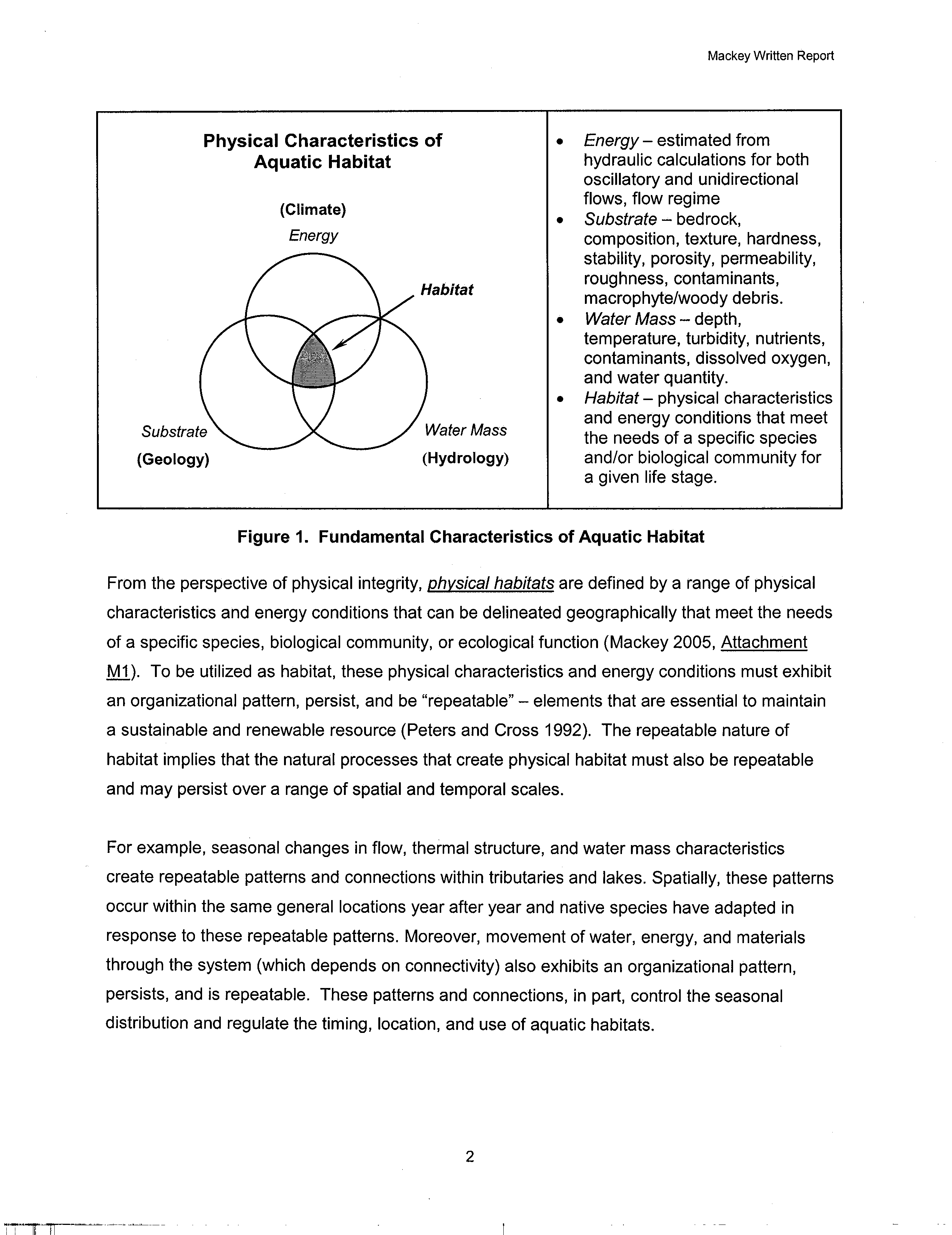
From the perspective of physical integrity,

physical habitats

are defined by a range of

physical characteristics and energy conditions that can be delineated geographically that meet the

needs of a specific species, biological community, or ecological function. To be utilized as

habitat, these physical characteristics and energy conditions must exhibit an organizational

3

I

---

pattern, persist, and be "repeatable" - elements that are essential to maintain a sustainable and

renewable resource. For example, seasonal changes in flow, thermal structure, and water mass

characteristics create repeatable patterns and connections within tributaries and lakes. These

patterns and connections, in part, control the seasonal distribution and regulate the timing,

location, and use of aquatic habitats.

Also critically important is the pattern and juxtaposition of different types of habitat. For

example, successful recruitment of fish will not occur if spawning habitat is not connected to

suitable nursery and forage habitats. Nursery and forage habitats provide sheltered areas where

larval and young-of-the-year (YOY) fish can feed and grow with minimal disturbance. Without

access to adjacent nursery areas, potential spawning sites are nothing more than substrate areas

with physical characteristics that mimic those of active spawning sites.

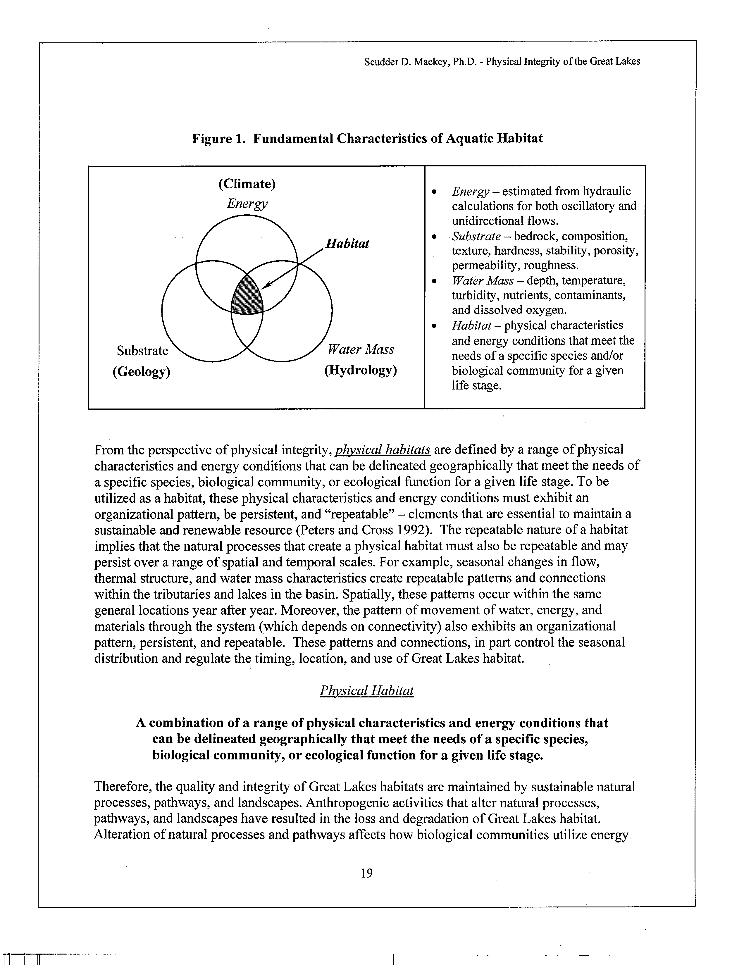
There are three major classes of variables that must be considered when assessing aquatic

habitat - 1) energy (flow regime), 2) substrate (composition, texture, structure), and 3) water

mass characteristics (water chemistry, water quantity). All of these variables must be spatially

and temporally connected by physical and biological

processes

in ways that support diverse

aquatic communities (see Figure 1 - Attachment 2). Biological characteristics are also an

important element of aquatic habitat, but will not be discussed in detail in this testimony and are

not included in Figure 1.

In a paper published in 1998, Yoder and Rankin made the point that the almost myopic

focus on water chemistry, point sources, and contaminants by many regulatory agencies has led

to an "incomplete foundation in water resource policy and legislation." Yoder and Rankin 1998

go on to state:

"Because biological integrity is influenced and determined by

multiple

chemical, physical, and biological factors, a singular strategy

4

I

---

emphasizing the control of chemicals

alone

does not assure the

restoration of biological integrity."

This statement serves as an appropriate backdrop for the testimony to follow.

UAA Methodology

The identification of Aquatic Life Use designations and the classification of waterway

reaches into the appropriate use categories are crucial to the successful conduct of a Use

Attainability Analysis (UAA) process. The process by which the Aquatic Life Uses are defined

and applied to waterways undergoing a UAA is the foundation for establishing appropriate water

quality standards. Ideally, the UAA provides a scientific basis to develop attainable designated

water uses that are based on a comprehensive integrated assessment of the physical, chemical

and biological conditions of a water body (USEPA, 1994). This assessment should include an

integrated analysis of current physical habitat, flow regime, temperature, water quality, and

existing aquatic communities.

The purpose of this integrated assessment is to determine whether existing or improved

conditions can be supported by changes in beneficial use and/or associated criteria. Thus, the

methodology used in defining and assigning uses for a specific waterway should be transparent,

scientifically based, and documented accurately, clearly, and completely. Unfortunately, the

CAWS UAA Report and supporting documents submitted by IEPA in this rulemaking effort do

not meet these criteria and contain data errors and flaws in the methodology used to develop the

proposed Aquatic Life Use designations.

Aquatic Life

Use Designations

IEPA has proposed to eliminate the current use designations that have been in place since

1972, and supplant them with a tiered system of Aquatic Life Uses supposedly based, in part, on

inferred relationships between physical habitat as characterized by Qualitative Habitat

5

I

---

Evaluation Index (QHEI) scores, and the Ohio boatable Index of Biotic Integrity (IBI), which

characterizes the health of the existing fish community. These new Aquatic Life Use tiers were

based on a comparison of IBI percentile scores and QHEI scores at each sample location.

Review of the QHEI and IBI scores revealed significant errors and uncertainties in the data, and

the methods used to compare the QHEI and IBI scores found in Figure 5-2 of the UAA Report

are not scientifically valid.

By focusing almost exclusively on the IBI metrics and percentiles, IEPA did

not

provide

an integrated analysis of physical habitat, flow regime, temperature, water quality, and existing

aquatic communities in their assessment of the CAWS. Specific issues that I will discuss

include: (1) sampling design, (2) significant problems using the QHEI for CAWS, (3) errors and

uncertainty in the data, and (4) fatal flaws in the Aquatic Life Use designation methodology.

1. There

are significant limitations in the current sampling design.

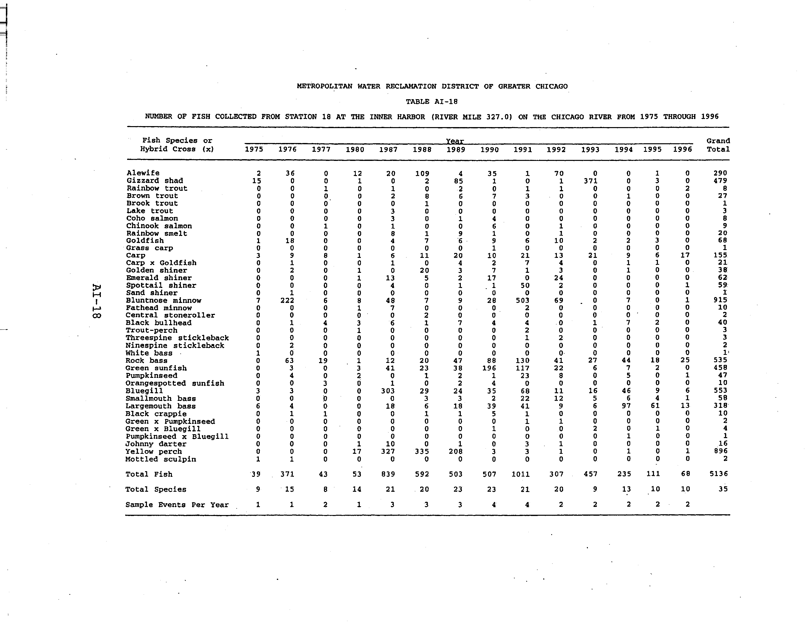
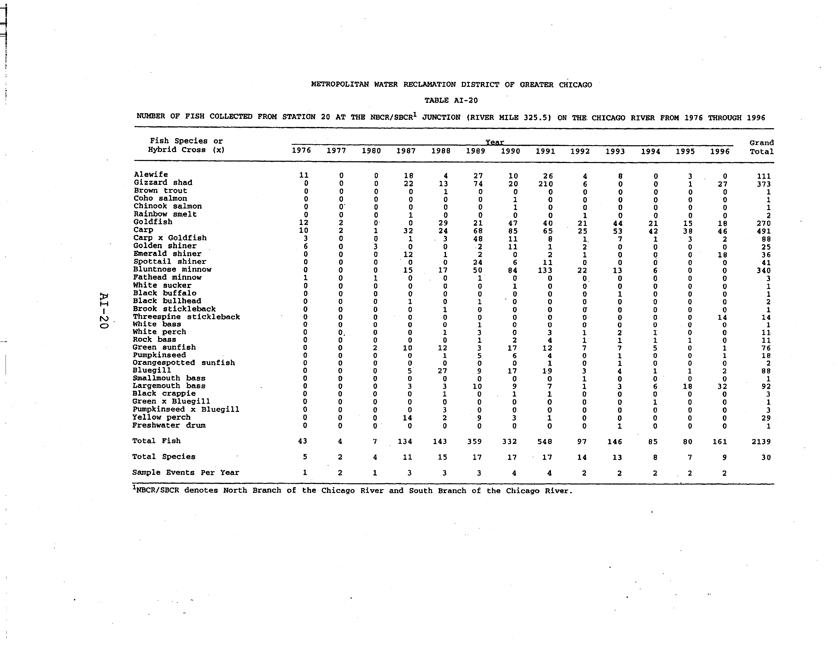
In the physical habitat assessment summarized by Rankin in 2004 (IEPA filing

Attachment R), QHEI values were calculated for 20 sites within the CAWS. These sites were

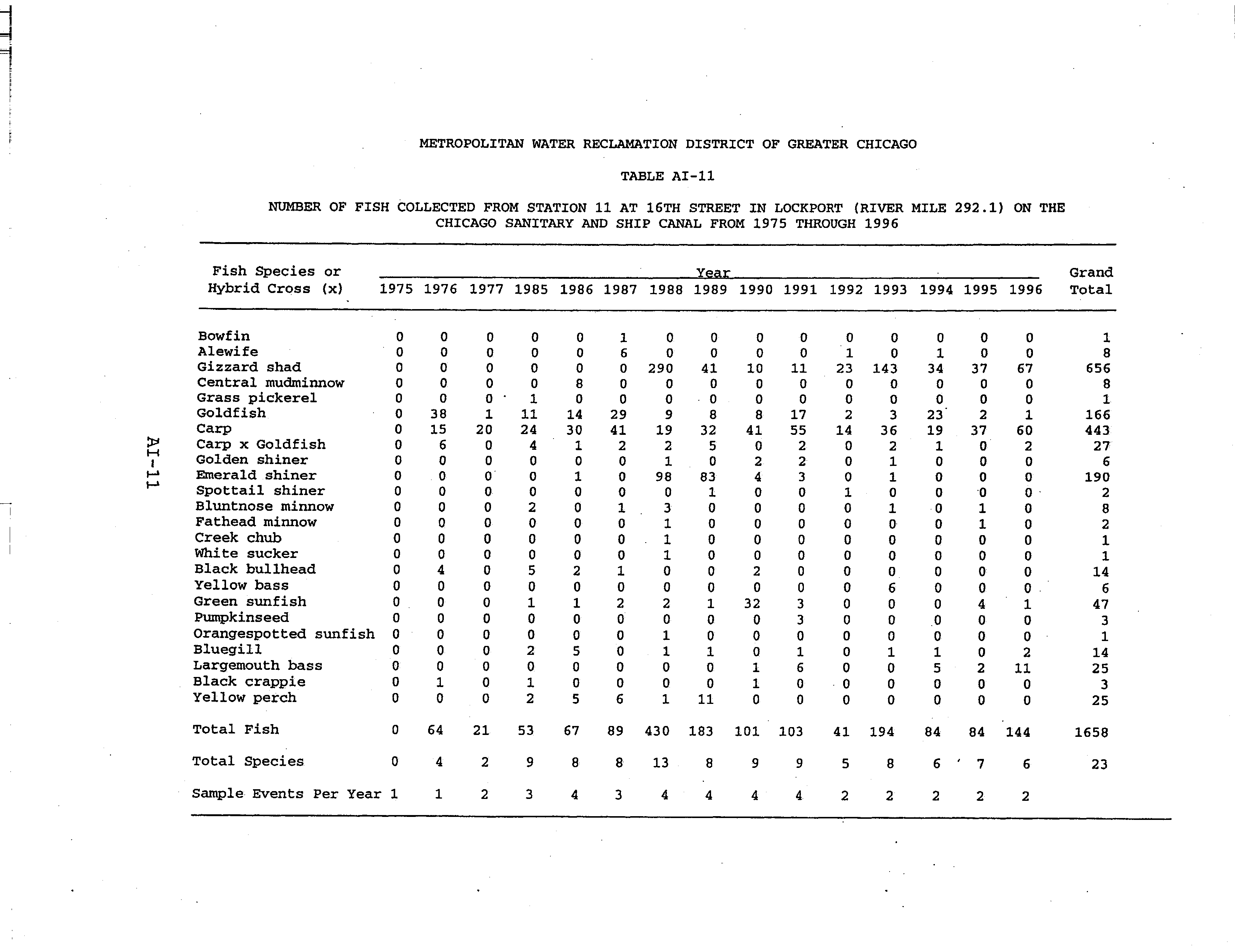
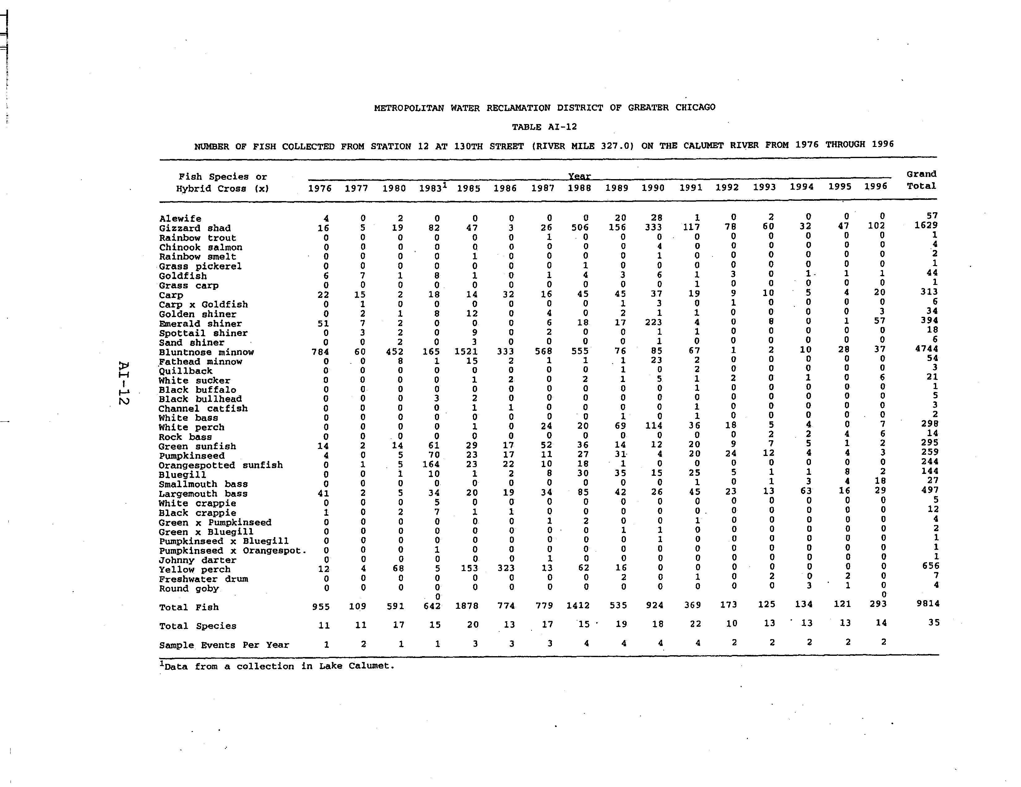
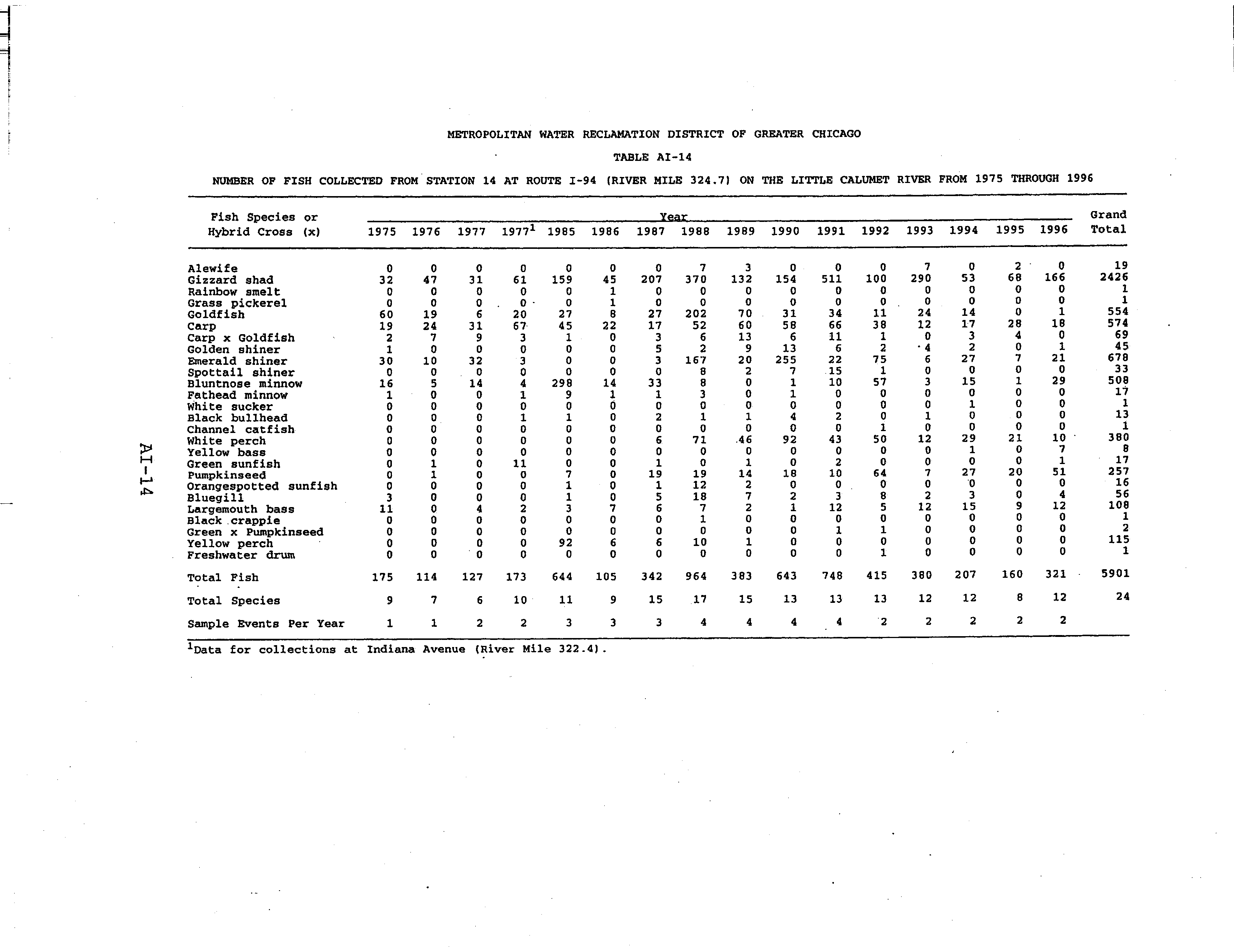
selected based on the availability of long-term fish sampling data made available by the

MWRDGC. The spatial distribution of these sites

was not

based on an appropriate statistical

sample design or consideration of inferred physical habitat processes or characteristics. Distances

between sampling sites ranged from 0.5 miles (0.8 km) to 15.8 miles (25.4 km), with a mean

sampling distance of 4.3 miles (6.9 km). Clearly, gaps of up to 15 miles between sampling

points in the waterway can not be considered to be a comprehensive assessment of physical

habitat.

Moreover, portions of the CAWS were not included in the physical habitat assessment.

For example, IBI and QHEI metrics for Bubbly Creek were

not evaluated at all,

and QHEI

metrics were

not

calculated for the South Branch of the Chicago River. Even though the channel

6

I

---

morphology and flow characteristics of Bubbly Creek and the South Branch of the Chicago

River are

distinctly different

from each other, the CAWS UAA Report [on page 4-69] states that

Bubbly Creek and the South Branch have "similar" environmental characteristics and are

grouped together as the

same

channel in the Report.

Widely-spaced, traditional point sampling does not provide adequate data to document

the type, area, pattern, or juxtaposition of different types of aquatic habitat that may exist in the

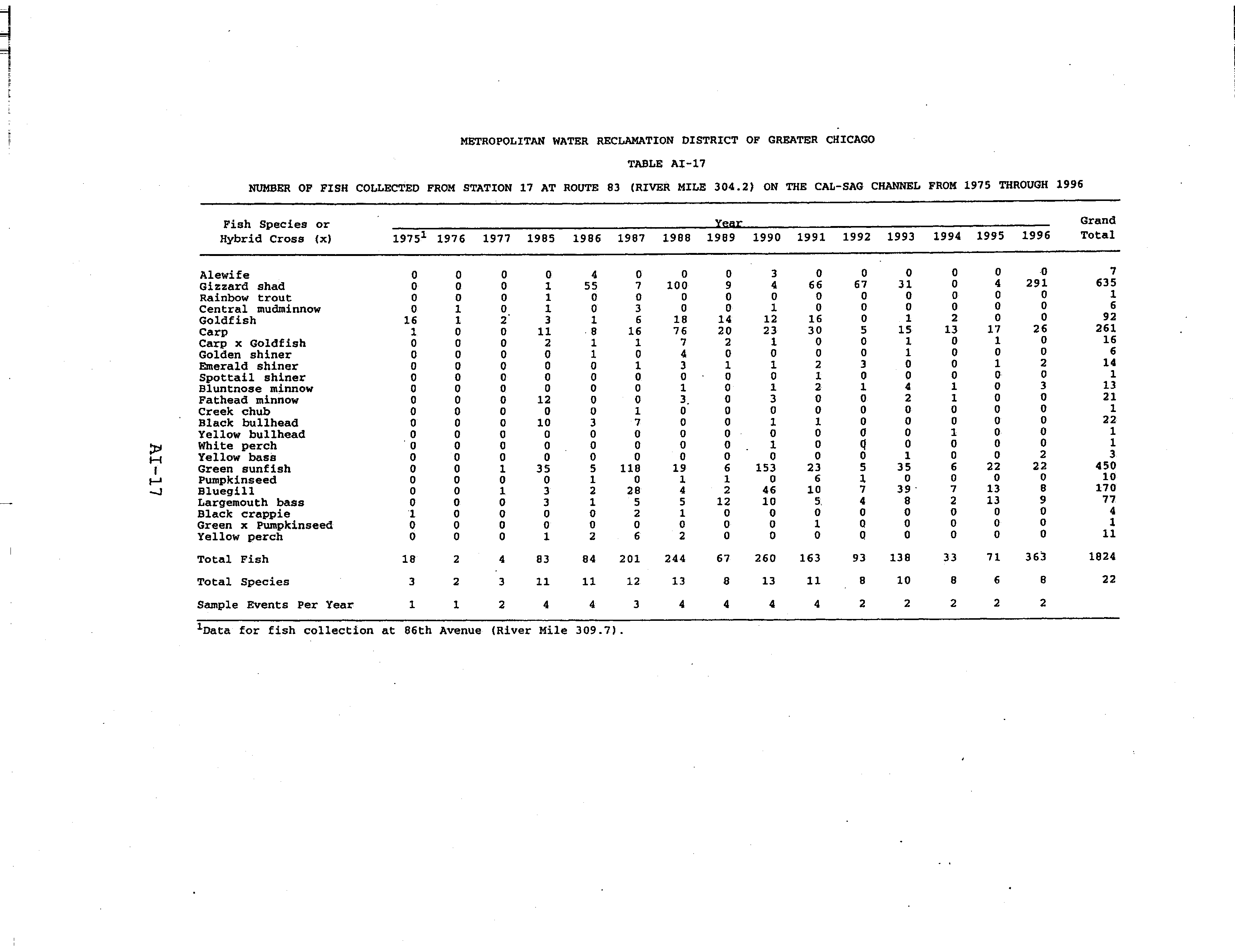
CAWS. For example, in the Calumet-Sag Channel, only

two

sites were evaluated using the IBI

and QHEI metrics,

and those sites were 10.7 miles apart.

These two sites form the basis for the

habitat assessment and Aquatic Life Use designation for the entire 16-mile channel length. The

limited number and wide spacing between habitat sampling sites is

a major

deficiency in the

CAWS UAA Report and IEPA Statement of Reasons.

IEPA purportedly considered shoreline and bank-edge (littoral) conditions for each of the

CAWS segments. This is surprising, because there has not been a comprehensive inventory and

assessment of shoreline or bank-edge habitat conditions for the CAWS, nor have there been

ecological studies of navigation or wave impacts on shorelines within the CAWS. Shoreline and

bank-edge areas provide spawning, nursery, and forage habitats necessary to sustain healthy,

propagating fish populations. As part of a comprehensive habitat assessment it would be

important to know what the relative percentage, location, pattern, and distribution of shoreline

types and bank-edge habitat are for each of the CAWS segments. This is particularly important

when assessing the pattern and juxtaposition of different types of aquatic habitats, which was

not

done

in the CAWS UAA Report or presented in the Statement of Reasons.

Even though bank-edge areas are regularly sampled by MWRDGC using electrofishing

equipment, the results are integrated and summarized across the entire channel segment to

7

I

---

calculate IBI scores at that sampling site. The reported IBI scores

may

be indicative of fish

utilization of bank-edge habitat, but the coarse sampling interval and lack of bank-edge habitat

data severely limits our ability to

draw any meaningful conclusions.

However, IEPA contends

that these shallow water bank-edge habitats in the Calumet-Sag Channel should be considered to

be spawning habitat, which is problematic given that

no direct data

are available to support that

contention. The lack of a comprehensive physical and biological assessment of existing shoreline

and bank-edge habitats is another

major

deficiency in the CAWS UAA Report and IEPA

assessment methodology.

2.

There

are significant

p

roblems applyin2

the QHEI to

low-gradient urbanized rivers

such as

the CAWS.

The QHEI protocol was developed to provide a measure of physical habitat quality and is

based on hydrogeomorphic metrics in

a natural

stream or river channel. There are six metrics

that comprise this index: substrate, instream cover, channel morphology, riparian zone/bank

erosion, pool/glide and riffle/run quality, and map gradient. The QHEI protocol is

not

designed

for use in low gradient, non-wadeable streams and rivers, in part because traditional sampling

approaches are inadequate to assess critical substrate, instream cover, or other metrics used in the

QHEI assessment protocol.

Within the CAWS, several of the key morphological metrics upon

which the QHEI scores are based are held constant or are not present. As a result, the QHEI

scores for the CAWS are calculated using sub-metrics that may be of

secondary importance

to

the attainment of a diverse, sustainable fish population. Embedded within the QHEI scoring

system is an

implicit

assumption that there is a relationship between flow hydraulics, channel

morphology, and the type and distribution of substrate materials. This assumption is not valid

for low gradient, urbanized, artificial channels such as the CAWS. Flows in the CAWS are

regulated, controlled by man-made structures, and are not natural. The channels in the CAWS

8

---

are stable (carved out of bedrock or artificially stabilized), and flows are generally decoupled

from substrates, i.e. coarse-grained substrates observed in the CAWS may not be dependent on

or controlled by flow. In summary, the QHEI protocol

was not

designed to be applied to a flow-

regulated artificial waterway system such as the CAWS.

3. There

are errors and uncertainty in the environmental data.

Careful review of the data and metrics calculated in the CAWS UAA Report reveals

errors and uncertainty in the QHEI data and fundamental errors in how the boatable IBI scores

were calculated. These errors call into question the reliability of the analysis and the resulting

recommendations. First, there is considerable uncertainty as to what the

actual

QHEI scores are

for the North Shore Channel and the Cal-Sag Channel Unfortunately, due to transposition errors

in the habitat assessment report by Rankin (IEPA Attachment R), the QHEI scores for the

reference site at Sheridan Road on the North Shore Channel and for sampling sites on the Cal-

Sag Channel were incorrectly stated (see Essig testimony, 4/23/08, page 192-193). If these

QHEI scores were transposed, then the QHEI score at the reference site is considerably lower (42

instead of 54), which places the high-quality reference site in the "poor" habitat category. Given

the significantly lower QHEI score, the Sheridan Road site

no longer

meets the criteria as an

appropriate high-quality reference site, and the boundaries of the proposed Aquatic Life Use

categories for the CAWS are invalid and should be redefined.

Note: Proper application of the Ohio Boatable IBI requires identification of high quality

reference streams which serve as yardsticks to measure the biological health in similar, regional

water bodies. A high-quality reference stream will have suitable habitats and a diverse, well-

balanced aquatic community using those habitats. These characteristics represent the highest

level of physical, chemical, and biological integrity that can be attained within these regional

systems.

9

---

If the QHEI scores that were originally reported

are correct,

then at the Cicero Avenue

sampling site on the Cal-Sag Channel, the box plot of IBI scores falls

below

the minimum line

for IEPA's Aquatic Life Use "A" waters, and a QHEI score of 37.5 is classified as a "poor"

habitat.

These data are consistent with the statement on page 4-92 of the UAA Report that the

fish IBI scores in the Cal-Sag Channel are classified as "poor to very poor" and the QHEI scores

are classified as "poor".

At the Route 83 sampling site, the IBI score appears to be on the

dividing line between IEPA's Aquatic Life Use "A" waters and Aquatic Life Use "B" waters, but

the QHEI score of 42 is still in the "poor" range.

The Cal-Sag Channel and the Chicago Sanitary and Ship Canal share similar physical

characteristics (for example, deep-draft waterway, limited shallow area along banks, high

volume of commercial navigation) except that there is more weathering of the channel walls in

the Cal-Sag Channel.

The weathering of the bank walls provides a slight shallow shelf with

limited habitat for fish. This difference explains the slightly higher QHEI scores in the Cal-Sag

Channel compared to the Chicago Sanitary and Ship Canal. Nevertheless, both waterways are

considered "poor" habitat according to the QHEI classification scale in Table 2 of Rankin's

habitat assessment report (IEPA Attachment R). The small amount of rubble from the crumbling

walls does very little to improve the overall physical habitat for fish and invertebrates in the Cal-

Sag Channel.

The decision to include the Cal-Sag Channel as a higher Aquatic Life Use "A" water is

not

defensible, because the habitat indices for both monitoring stations were in the poor range,

and the IBI percentile scores are below or at the bottom of the range established for IEPA's

Aquatic Life Use "A" tier. In fact, the minimum IBI scores observed at the two monitoring

stations in the Cal-Sag Channel are among the lowest in the CAWS.

10

---

Second, there are errors in the IBI scoring criteria listed in Table 4-11 of the CAWS

UAA Report [page 4-27]. In this table, the scores for the "fish numbers" metric have been

reversed. Instead of adding 5 points when there are less than 200 fish and 1 point when there are

greater than 450 fish, the opposite should have been done. This error tends to inflate the IBI

scores when fish densities are low.

Moreover, a special scoring procedure was incorrectly

applied to the CAWS data that is intended

only

for the Ohio

wadeable

IBI,

not

for the Ohio

boatable

IBI. Since the proposed Aquatic Life Use designations were based on these inflated IBI

scores,

all

of the Aquatic Life Use designations proposed for the CAWS need to be reconsidered

using the corrected IBI scores.

4.

There

are fatal flaws in the Aquatic

Life

Use designation methodology.

The method used to compare the QHEI and IBI scores found in Figure 5-2 of the UAA

Report are not scientifically valid. First, by plotting the IBI and QHEI scores on the same graph,

there is an implicit assumption that there is a one-to-one correspondence of IBI scores to QHEI

scores, even though this is clearly not the case. Rankin in his 1989 paper states that "using the

QHEI as a site-specific predictor of IBI can vary widely depending on the predominant character

of the habitat of the reach".

Second, IEPA adopted the approach used in the CAWS UAA Report, and

in that report,

the lines used to delineate the Aquatic Life Use categories are

based solely on the percentile IBI

scores.

Specifically, the Aquatic Life Use categories are delineated using the 75th percentile of

the IBI scores at the reference site (NSC Sheridan Road) and the 75th percentile of the IBI scores

from the entire waterway. Neither the CAWS UAA Report nor the materials supporting the

proposed rule provide any justification (biological or otherwise) for using the 75th percentile IBI

as a threshold.

11

---

Third, Figure 5-2 gives the impression that

both

biotic (IBI) and habitat (QHEI) indices

were utilized in formulating the Aquatic Life Use tiers, and that observed IBI scores were

consistent with the corresponding QHEI scores for selected reaches of the CAWS. However, the

range shown on the vertical axis for the IBI score is 12-38, even though the entire range of

possible IBI scores is from 12-60. On the QHEI score axis, the scale includes the entire range of

possible QHEI scores from 0 to 100. By plotting the IBI scores in this way, it is possible to

"adjust" where QHEI scores line up on the graph relative to the 75th percentile IBI line. In other

words, the scale on the IBI axis can be adjusted or scaled up or down to

arbitrarily

fit the QHEI

data to whatever IBI percentile is desired (what QHEI score would you like it to be?).

QHEI thresholds determined using this methodology are

arbitrary

and

scientifically

invalid.

The ability to arbitrarily shift the IBI percentile lines relative to the QHEI data in Figure

5-2 invalidates the justification provided for IEPA's use of a QHEI score of 40 as a lower

boundary for Aquatic Life Use "A" waters rather than a QHEI score of 45 as recommended by

Rankin in 2004 (IEPA Attachment R). To summarize, even though Figure 5 -2 appears to be

correct, any comparisons made between IBI and QHEI scores using this methodology are

not

scientifically valid.

Finally, it is stated in IEPA's Statement of Reasons that Aquatic Life Use "B" waters "are

capable of maintaining aquatic-life populations predominated by individuals of tolerant types..."

and Aquatic Life Use "A" waters "are capable of maintaining aquatic-life populations

predominated by individuals of tolerant or intermediately tolerant types..."

During cross-

examination of IEPA, efforts to elucidate a more detailed description of desired aquatic

communities for the CAWS were unsuccessful (see Smogor testimony, 3/10/08, pages 10-12).

The lack of a desirable (or expected) fish and benthic invertebrate species list is somewhat

12

---

surprising, because one would think that a description of the desired aquatic communities for

Aquatic Life Use "A" waters and/or Aquatic Life Use "B" waters would be useful to determine

if, and when, desired Aquatic Life Uses are actually attained. If we can't describe the biological

community that is potentially attainable, then how do we know that it doesn't already exist?

In summary, based on the aforementioned deficiencies, the Aquatic Life Use categories

and designations as proposed in IPCB R08-9 need to be reconsidered using a more transparent,

scientifically-based methodology.

At a minimum, the IEPA must first review and correct any

inaccuracies in the environmental data

before

using that data to delineate proposed Aquatic Life

Use waters for the CAWS. Further clarification is also needed regarding their approach and

basis for defining Aquatic Life Use tiers and designations. IEPA's current methodology relies

almost exclusively on the boatable IBI scores and does

not

adequately consider physical habitat,

flow regime, or existing aquatic communities. If these elements are not incorporated into IEPA's

analysis, the methodology must be judged as incomplete, arbitrary, and poorly founded in

science.

The Proposed

Water

Ouality Standards

Will Not Achieve

Designated Uses

In the Statement of Reasons, the IEPA hypothesizes that increased DO and reductions in

temperature will significantly improve fish diversity and community structure within the CAWS.

This implies that IEPA has determined that DO and elevated temperatures are the primary

stressors limiting the biological potential of aquatic communities in the CAWS. In their

submittals, the IEPA has not provided evidence that these are indeed the primary factors that

limit the development of a diverse, sustainable fish community in the CAWS. I would ask why

IEPA didn't compare readily available DO data with fish richness metrics from the CAWS to

demonstrate that the proposed increases in DO would

indeed

result in a significant increase in

fish richness and diversity. This is another deficiency in the IEPA assessment methodology.

13

---

Other non-water quality related parameters could also be limiting the biological potential

of the CAWS.

Examples include

,

but are not limited to:

•

Physical limitations such as lack of shallow bank-edge habitats and riparian cover; lack of

instream habitat cover and diversity; lack of suitable substrates and substrate heterogeneity;

or altered flow regimes (flow and water levels);

•

Biological limitations such as limited primary productivity, degraded

macrobenthic

communities (food supply), predation, or lack of appropriate spawning and nursery habitats;

•

Chemical limitations such as legacy contaminants in the sediments; and

•

Functional limitations such as navigation (prop wash and turbulence, sediment resuspension;

waves) and conveyance of waste and flood waters (variable flow regime, water levels).

Other investigators have recognized these potential limitations as well. For example, the

MWRDGC in Report 98-10 concluded that a lack of diverse aquatic habitats is one of the major

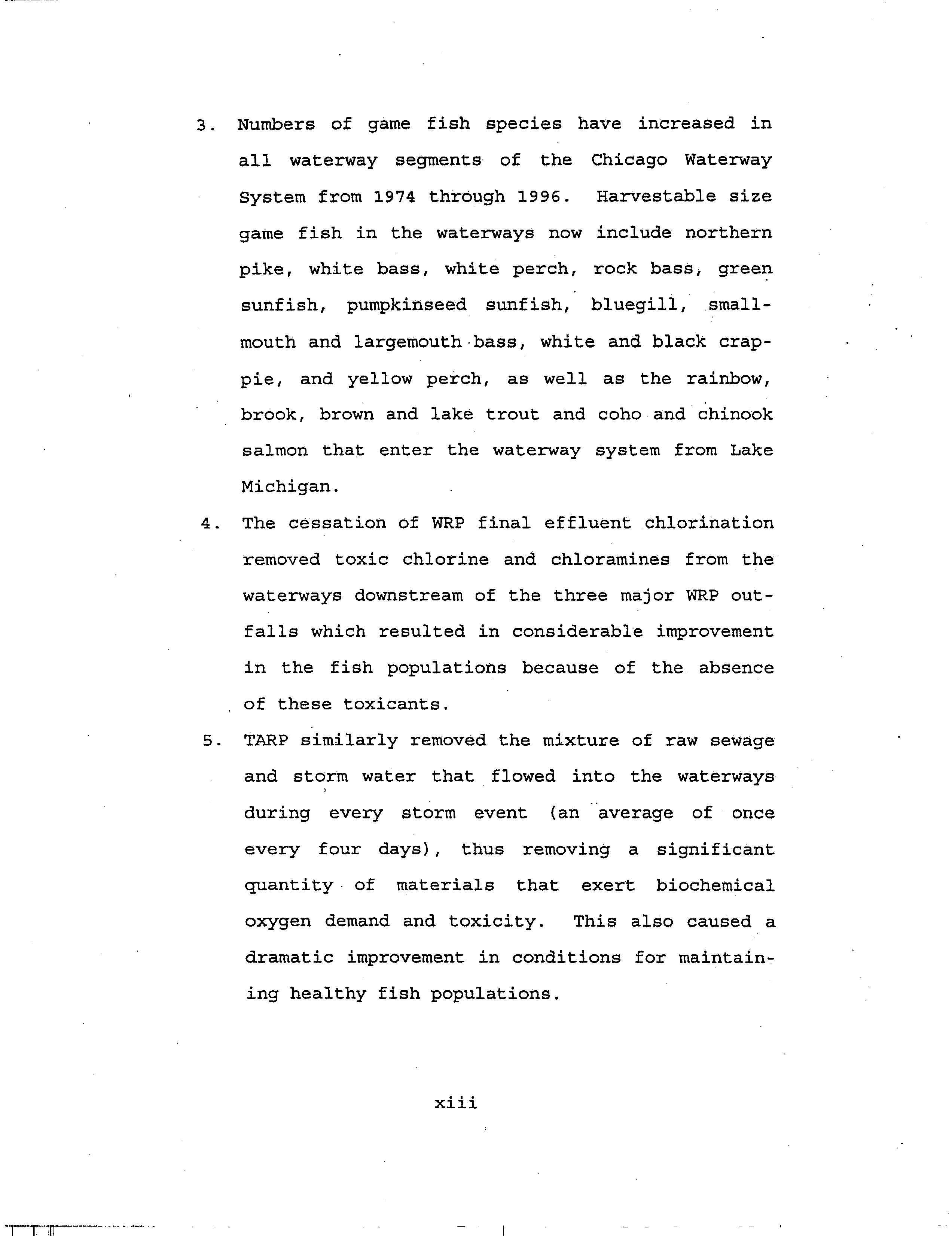
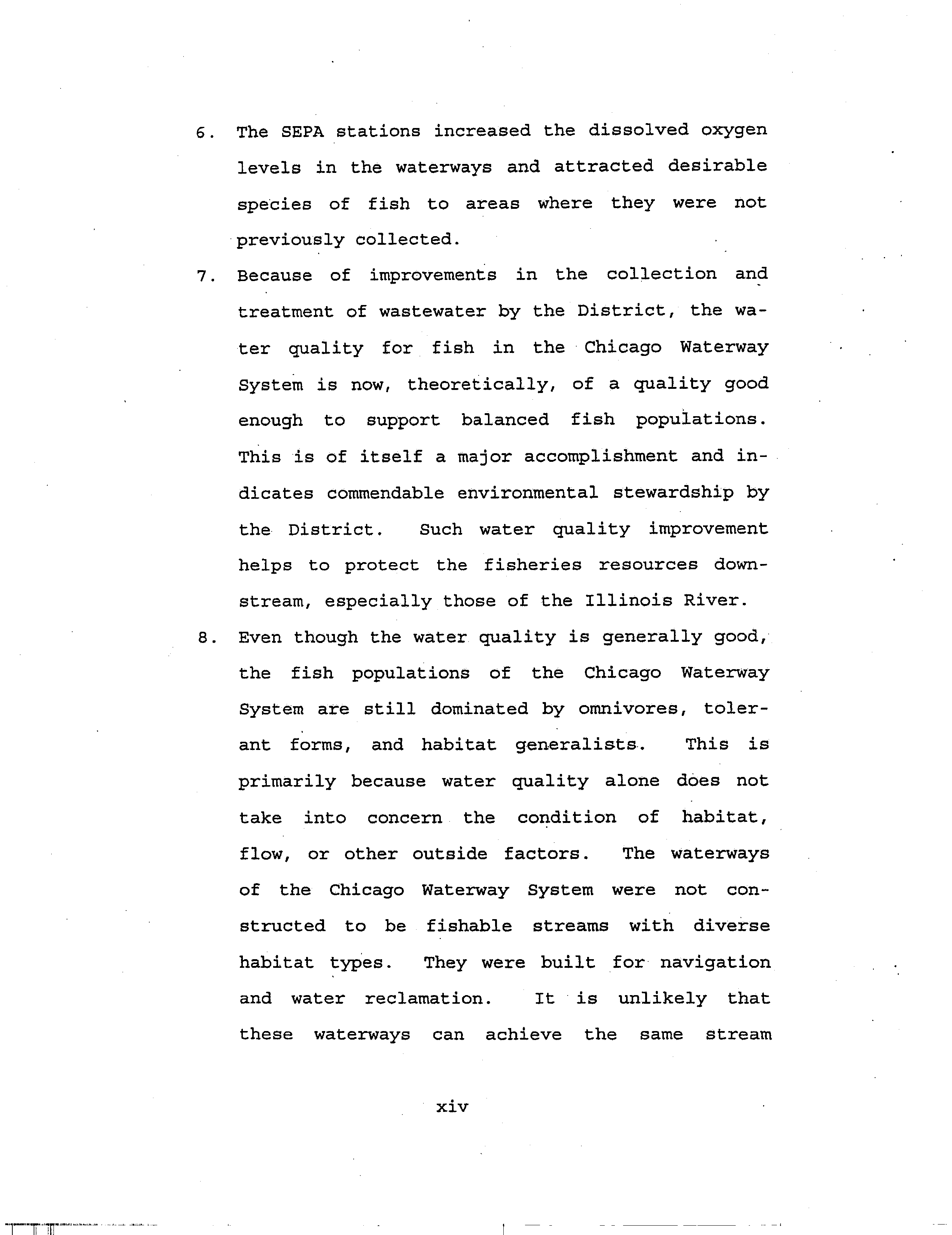
limiting factors affecting fish diversity and richness in the CAWS. Conclusion 8 of the report

states:

"Even though water quality is generally good, the fish populations of

the Chicago Waterway System are still dominated by omnivores,

tolerant forms, and habitat generalists. This is primarily because water

quality alone does not take into concern the condition of habitat, flow,

or other outside factors. The waterways of the Chicago Waterway

System were not constructed to be fishable streams with diverse

habitat types. They were built for navigation and water reclamation.

It is unlikely that these waterways can achieve the same stream quality

for fish as a natural habitat-rich waterway unless desirable fish habitat

is created..."

The CAWS UAA Report

also found that a lack of suitable habitat may be a major factor

that limits the attainment of diverse

,

sustainable fish communities

.

In fact the report on page 5-3

states:

"Improvements to water quality through various technologies, like re-

aeration may not improve the fish communities due to lack of suitable

habitat to support the fish populations. Unless habitat improvements

are made in areas like the CSSC, additional aeration may not result in

the attainment of higher aquatic life use."

14

I

---

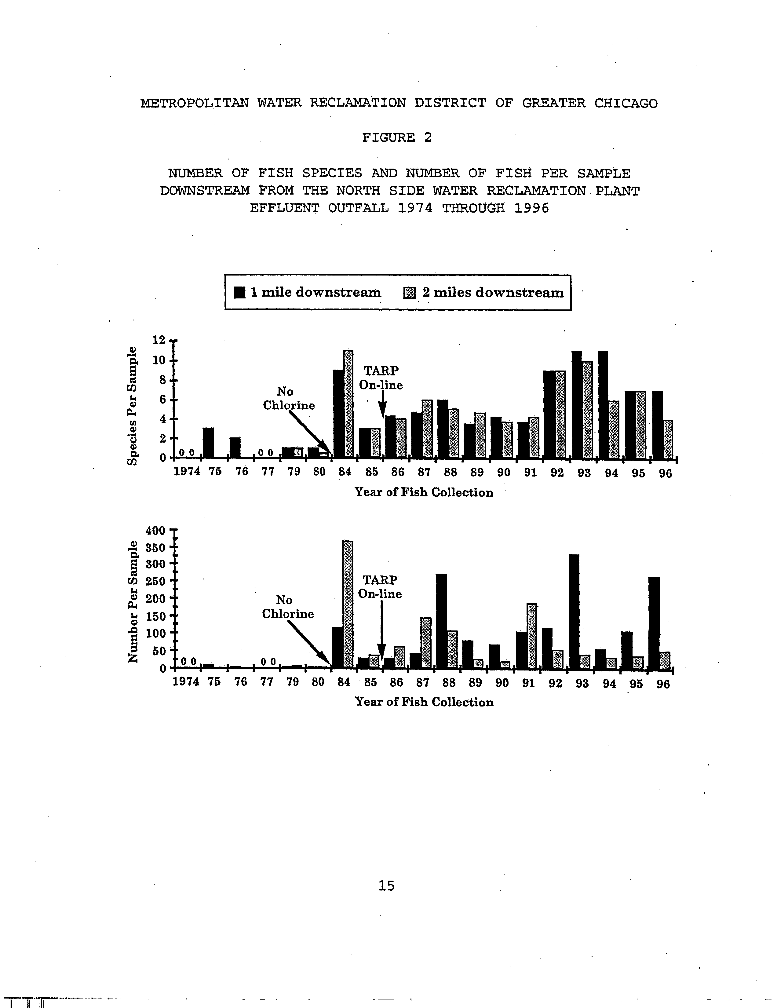
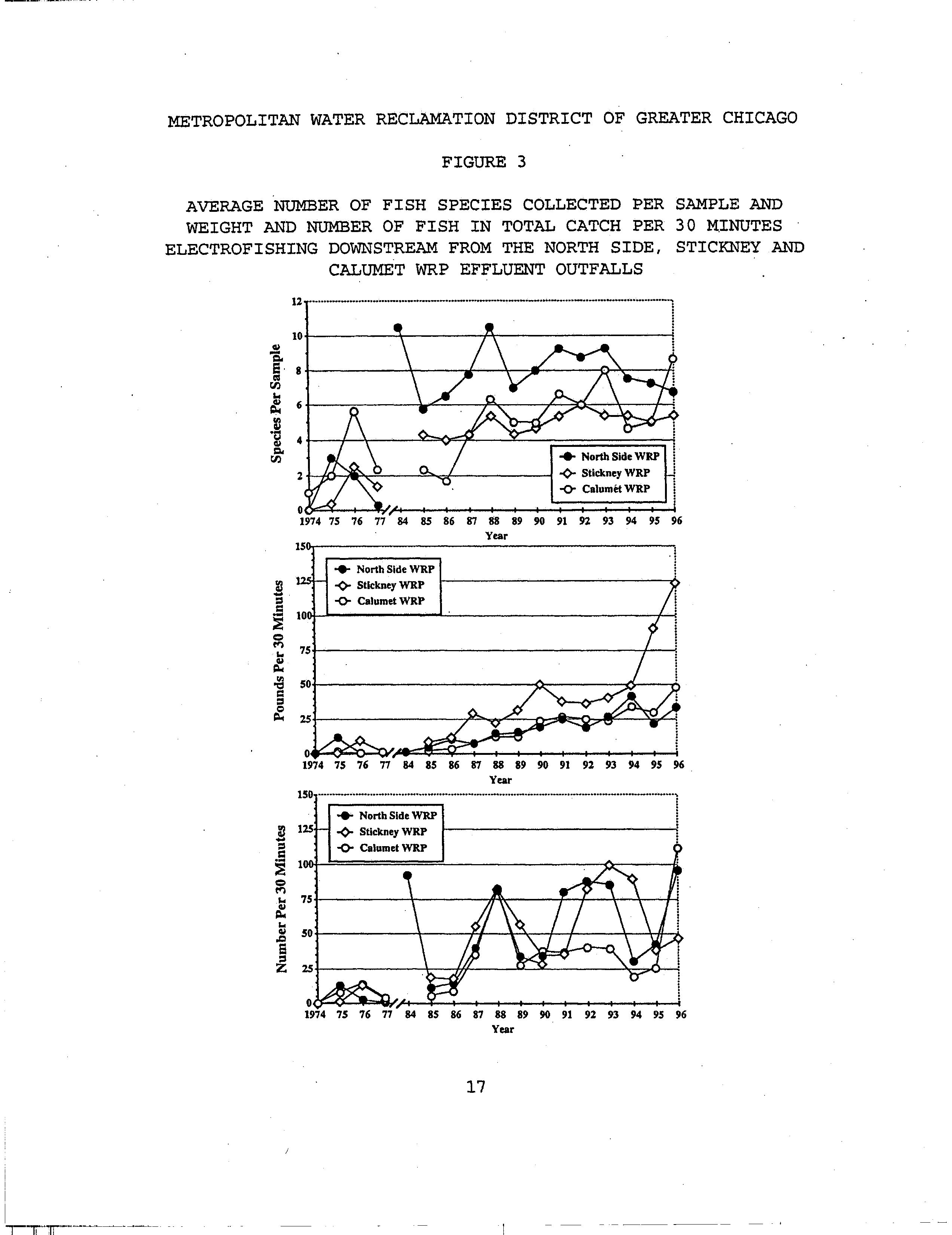
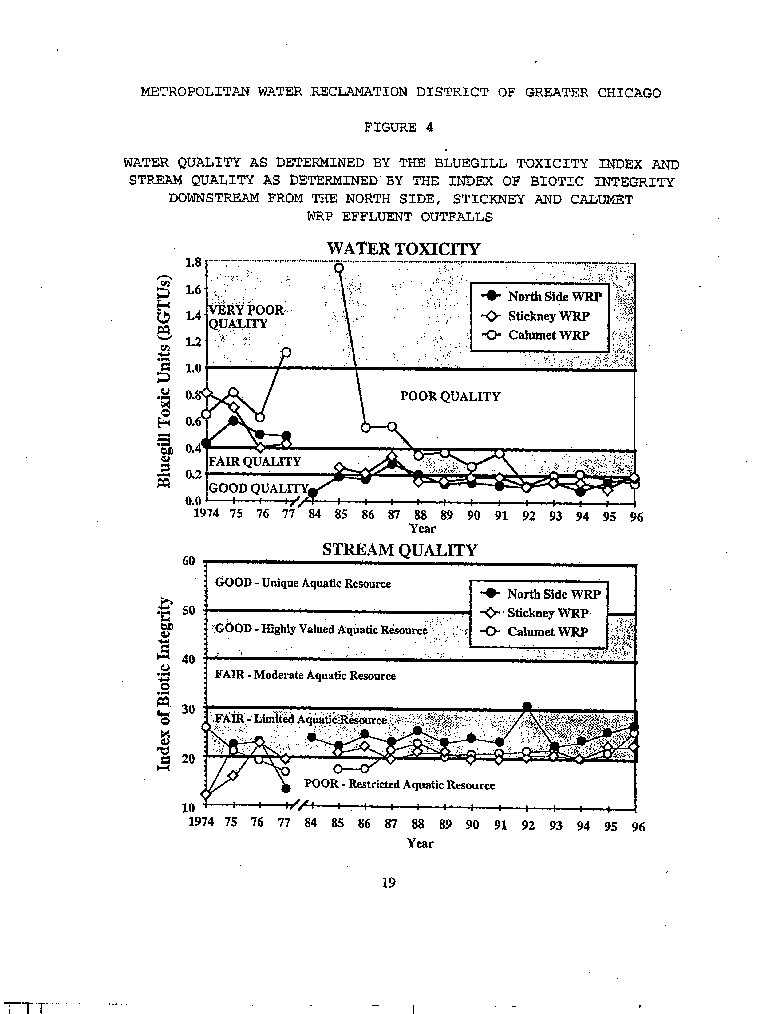
Multiple lines of evidence support the fact that water quality in the CAWS has

improved

significantly

over the past several decades and is now good enough to support the passage of fish

and other aquatic organisms to and from the Mississippi River and Great Lakes Basins via the

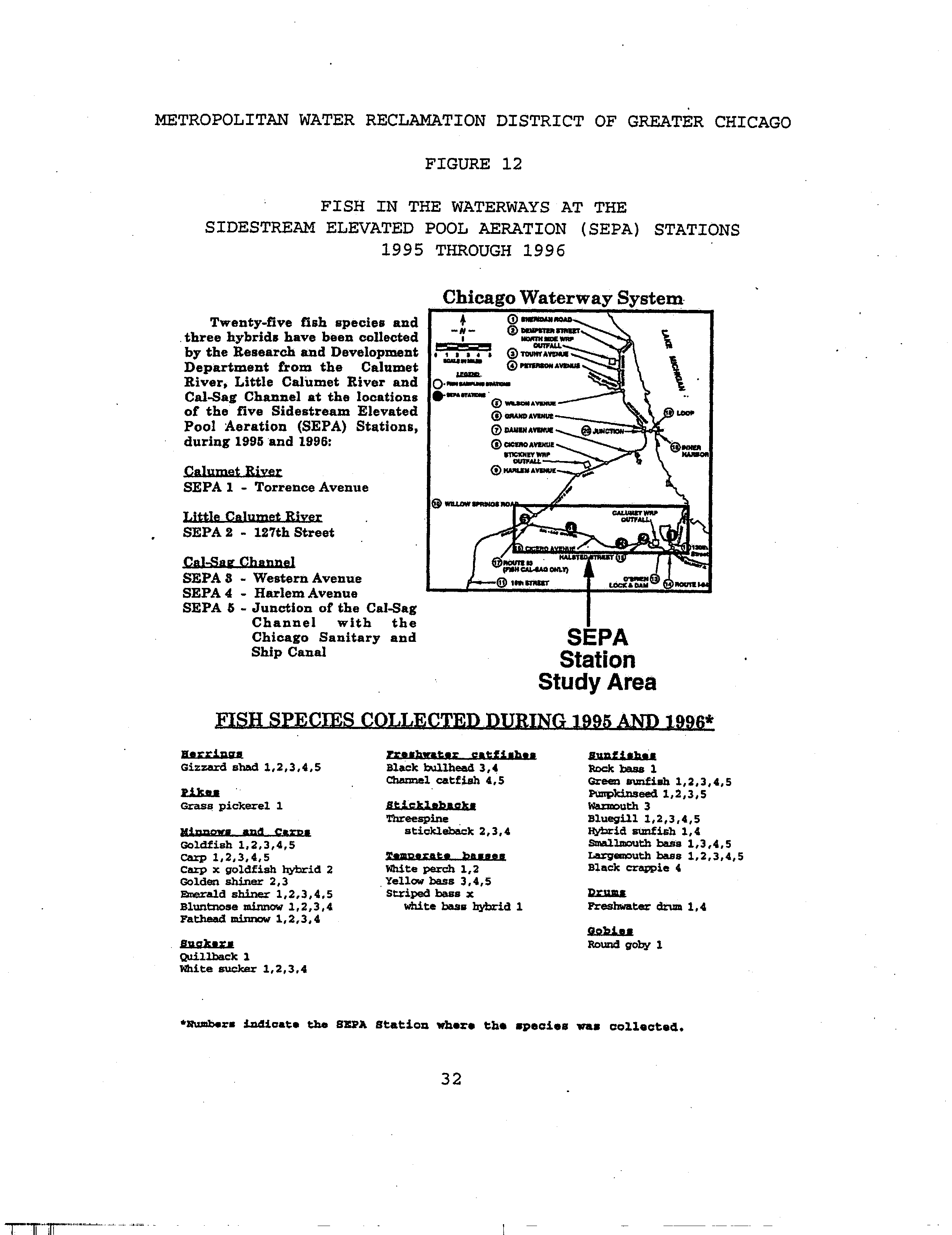
CAWS. For much of the CAWS, fish richness and diversity has improved markedly since

effluent chlorination was terminated in 1984, the Tunnel and Reservoir Plan (TARP) came

online in 1985, and SEPA (aeration) stations improved DO levels in the Calumet River system.

Moreover, the existence of active angler groups and bass fishing tournaments on the

waterway also suggests that for many species, water quality (DO and temperature) for much of

the CAWS is

not a significant limiting factor.

Certainly there continue to be DO and temperature

limitations for other desirable, less-tolerant species (which are not specifically identified in the

UAA report or IEPA's statement of reasons), but if suitable habitats are not present, sustainable

populations of these species will not become established in the CAWS,

irrespective of how much

improvement there is in water quality.

A diverse benthic community is an important food source for young and adult fish. Lack

of an adequate benthic food supply could be a major limitation that is not necessarily related to

water quality or DO

,

but instead is caused by limitations in physical habitat

(

unnatural flow, lack

of suitable substrates

,

and poor sediment quality). In fact

,

fair to good Macroinvertebrate Biotic

Index (MBI) scores from the

"

in-water column

"

Hester Dendy samplers and

very

poor MBI

scores within CAWS sediments

(

Ponar grab samples

)

suggest that water quality improvements

may

already be sufficient

to support a more robust and diverse macroinvertebrate community if

suitable habitats were present in the

CAWS (

Wasik testimony).

In my opinion

,

the substantial investments needed for infrastructure to provide

incremental increases in DO and/or reductions in temperature will

not

yield a proportionate

15

---

biological response with respect to attaining sustainable fish communities and/or other beneficial

uses. The lack of diverse bank-edge and instream habitats within the CAWS may be a much

more significant limitation on the development of sustainable fish communities than current

levels of DO or temperature.

Without suitable habitat pattern and diversity, sustainable

populations of these species can not be established

irrespective of how much improvement there

is in water quality.

In fact, opportunities to improve physical habitat structure and increase

habitat diversity in selected reaches within the CAWS may yield a much more significant

biological response than system-wide improvements in DO and temperature.

Need for an Alternative Strategy to Generate a Comprehensive Habitat Assessment

Integrating all Fundamental Habitat Characteristics Necessary to Maximize Productive

and Ecological. Capacity of the CAWS

After reviewing the CAWS UAA Report, IEPA's proposed rule R08-9, and supporting

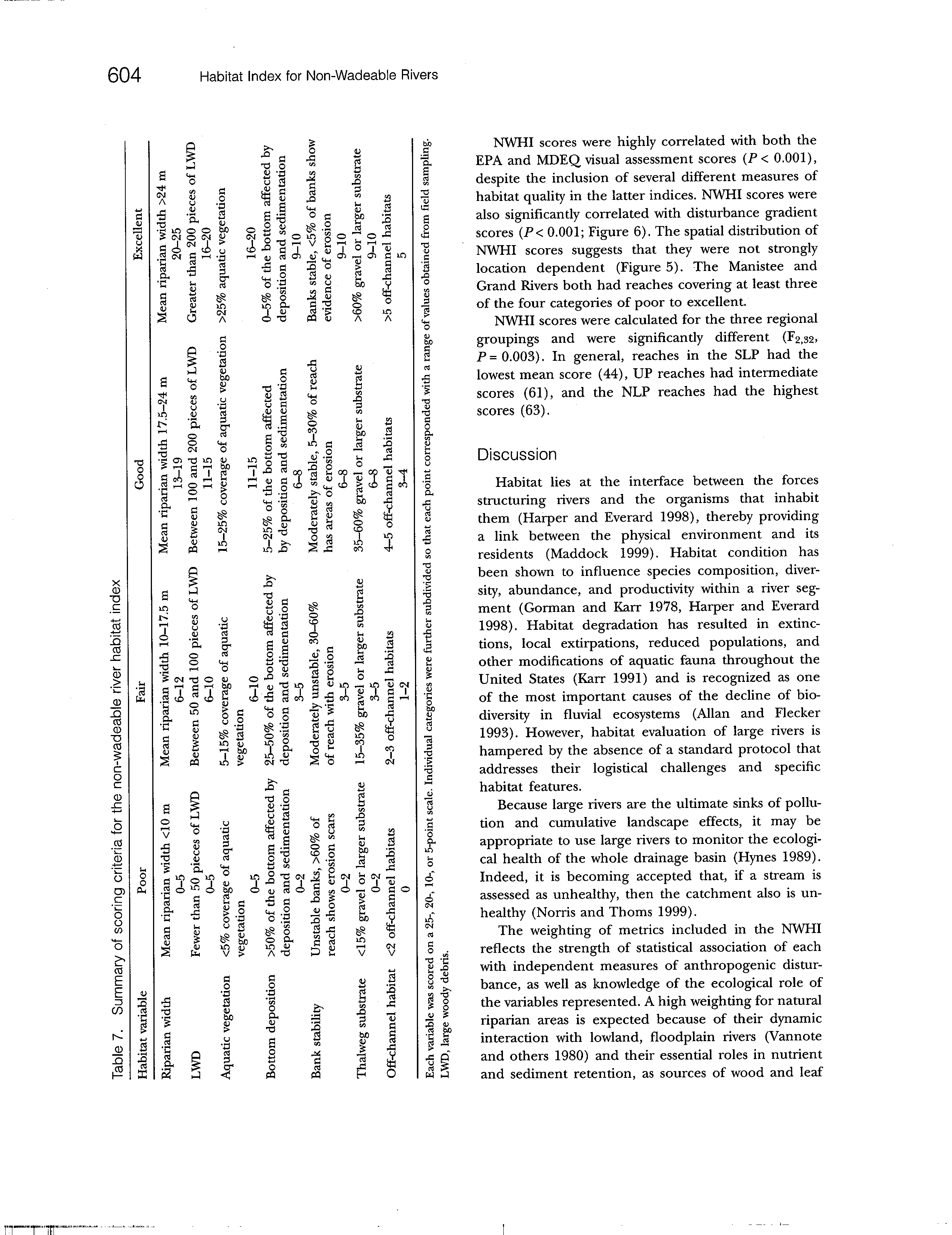
documentation, it becomes clear that there are major gaps in the CAWS environmental datasets,

especially with respect to physical habitat, spatial and temporal sampling, and the need for new

indices designed specifically to assess and summarize habitat and biological conditions in low-

gradient, non-wadeable, highly altered, urban streams and rivers.

Many of the major deficiencies

in IEPA's approach are listed in Table 1 (Attachment 3)

Recognizing the data gaps and limitations in the CAWS UAA Report, the MWRDGC in

the fall of 2007 issued a request for proposals entitled "Habitat Evaluation and Improvement

Study" designed to address many of the data gaps and deficiencies listed in Table 1. This study,

which is funded by the MWRDGC, is anticipated to be completed by summer 2009. As part of

this project, historical environmental data and newly collected environmental data will be

integrated into a comprehensive GIS package that will enhance accessibility and facilitate

analysis of CAWS environmental datasets.

16

---

The Habitat Evaluation and Improvement Study that is currently underway will follow a

scientifically sound, peer-reviewed, methodology for development of habitat indices in non-

wadeable rivers (Wilhelm,

et al.,

2005) to develop a CAWS-specific physical habitat index. This

index will be designed to differentiate habitat quality in the CAWS, where habitat variability is

relatively limited, especially within reaches. The study will make extensive use of existing biotic

and habitat data collected by MWRDGC between 2001 and 2007, supplemented with detailed

fish,

macroinvertebrate, water quality, and habitat data from 30 CAWS sampling stations in

2008. These data will be further augmented by digital bathymetric and shoreline video covering

the entire CAWS.

Robust multivariate statistical methods will be used to reduce the data and to identify the

most important fish and habitat variables in the CAWS. This approach will provide the strongest

relationships between fish and habitat, which is essential for understanding the ability of fish to

thrive in the CAWS. When completed, the CAWS habitat index will be applied to the entire

CAWS system. Furthermore, other important factors affecting fish will be considered in

evaluating habitat quality in the CAWS, including sediment chemistry and navigation impacts.

This study will create opportunities to develop linkages between physical habitat, water

quality, and aquatic communities in the CAWS. These linkages can then be used to

systematically (and scientifically) evaluate and manage for potential Aquatic Life Uses for

various segments of the CAWS, at scales much finer than had been previously possible.

Conclusions

Given the many deficiencies in the habitat data and lack of an appropriate science-based

methodology to designate Aquatic Life Use waters, the IEPA filing of proposed rule R08-9 and

17

17

1

---

associated DO and temperature criteria is premature.

Moreover, in my opinion, the protections

proposed in rule R08-9 are unnecessary and will not measurably enhance fish community

structure, aquatic diversity, or beneficial uses within the CAWS. It is not at all evident that the

substantial investments needed for infrastructure to provide incremental increases in DO and/or

reductions in temperature will result in attainment of Aquatic Life Uses that are different from

what already exist.

The ongoing Habitat Evaluation and Improvement Study is designed to address many of

the deficiencies highlighted in this testimony. This study will be completed by the end of this

calendar year with data and results available summer 2009. By integrating the results of this

study with other CAWS datasets, it should be possible to perform a comprehensive, integrated

assessment of the physical, chemical, and biological integrity of the CAWS. The objective

would be to identify the most efficient and cost-effective means to further protect and enhance

Aquatic Life Use waters and associated beneficial uses in the CAWS. It would then be

appropriate to move forward once this work has been completed.

I

would like to thank the Illinois Pollution Control Board for the opportunity to present

this testimony. I hope that the Board will carefully consider this testimony and act accordingly.

18

I

---

Testimony Attachments

1.

Resume: Scudder D. Mackey, Ph.D.

2.

Figure 1 Physical Characteristics of Aquatic Habitat

3.

Tab 1 e 1 Data Availability, Metrics, and Methods

4.

Written Report: Scudder D. Mackey, Ph.D.

References

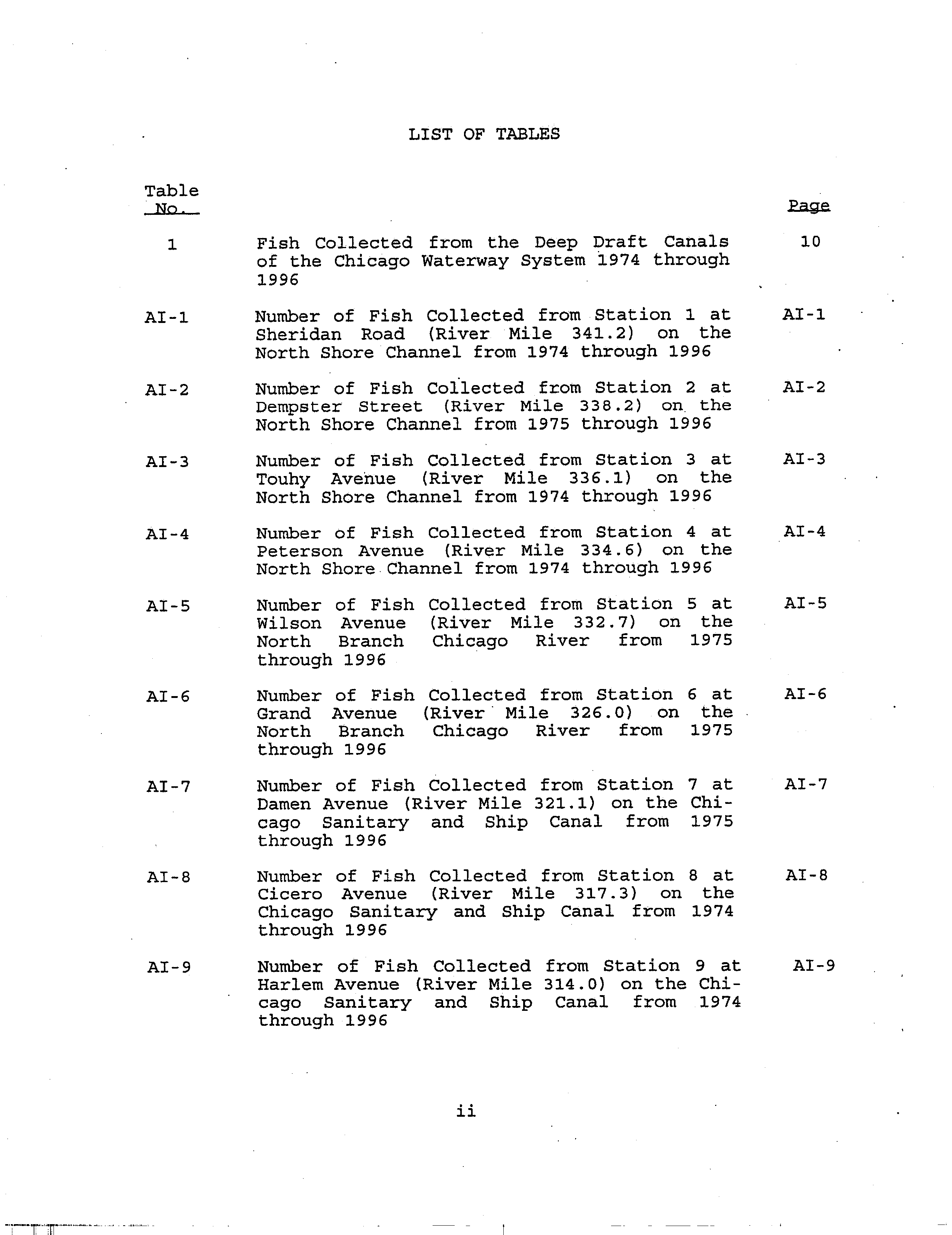
MWRDGC. 1998. A Study of the Fisheries Resources and Water Quality in the Chicago

Waterway System 1974 through 1996. Report 98-10

Rankin, E.T. 2004. "Analysis of Physical Habitat Quality and Limitations to Waterways in the

Chicago Area". Center for Applied Bioassessment and Biocriteria, IEPA Attachment R

Rankin, E.T. 1989. The Qualitative Habitat Evaluation Index (QHEI), Rationale, Methods, and

Application.

Ohio EPA, Division of Water Quality Planning and Assessment, Ecological

Assessment Section, Columbus, Ohio.

USEPA. 1994. Water Quality Standards Handbook, Second Edition. Office of Water Regulations

and Standards, Washington, D.C. EPA 823-B-94-005a, August 1994.

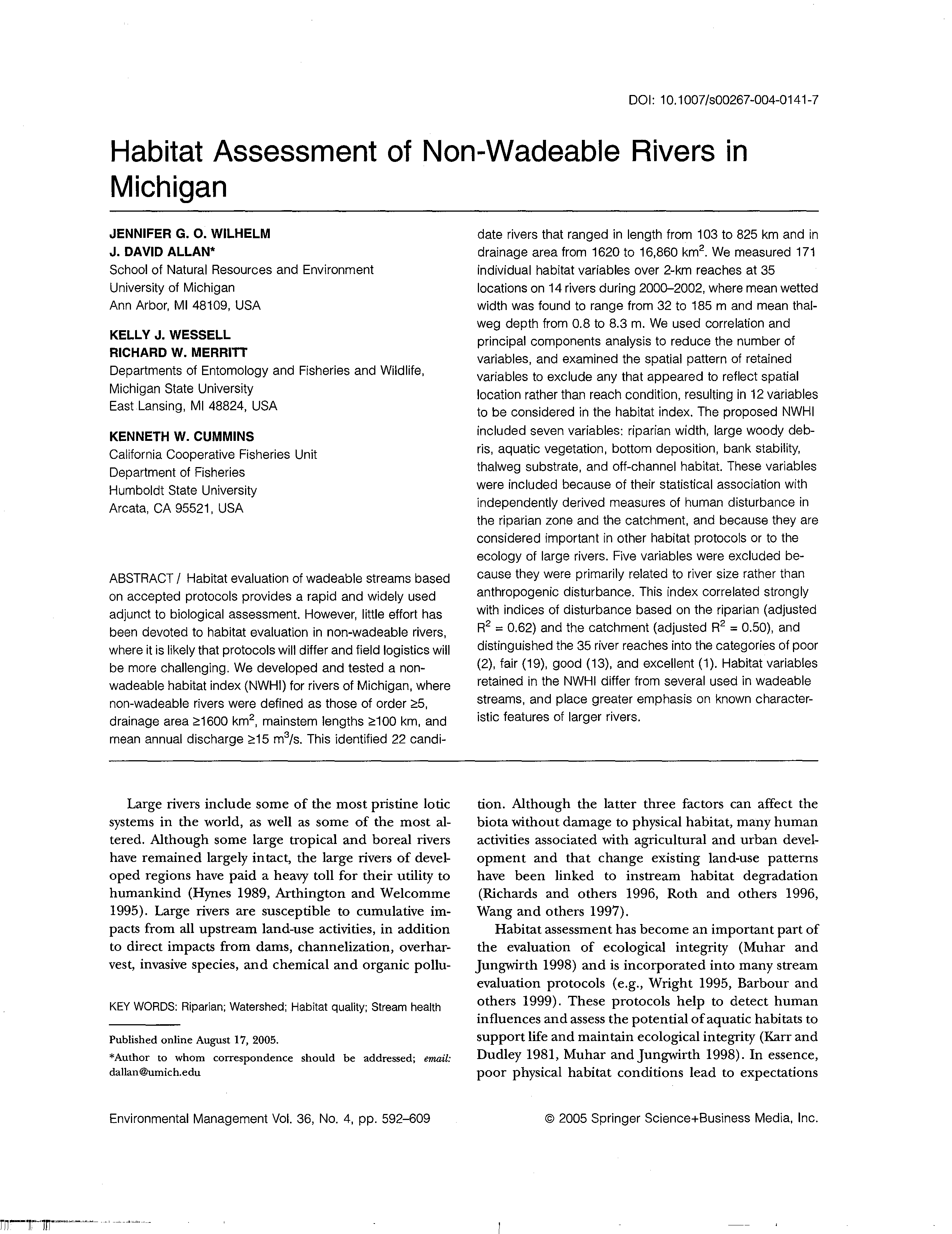
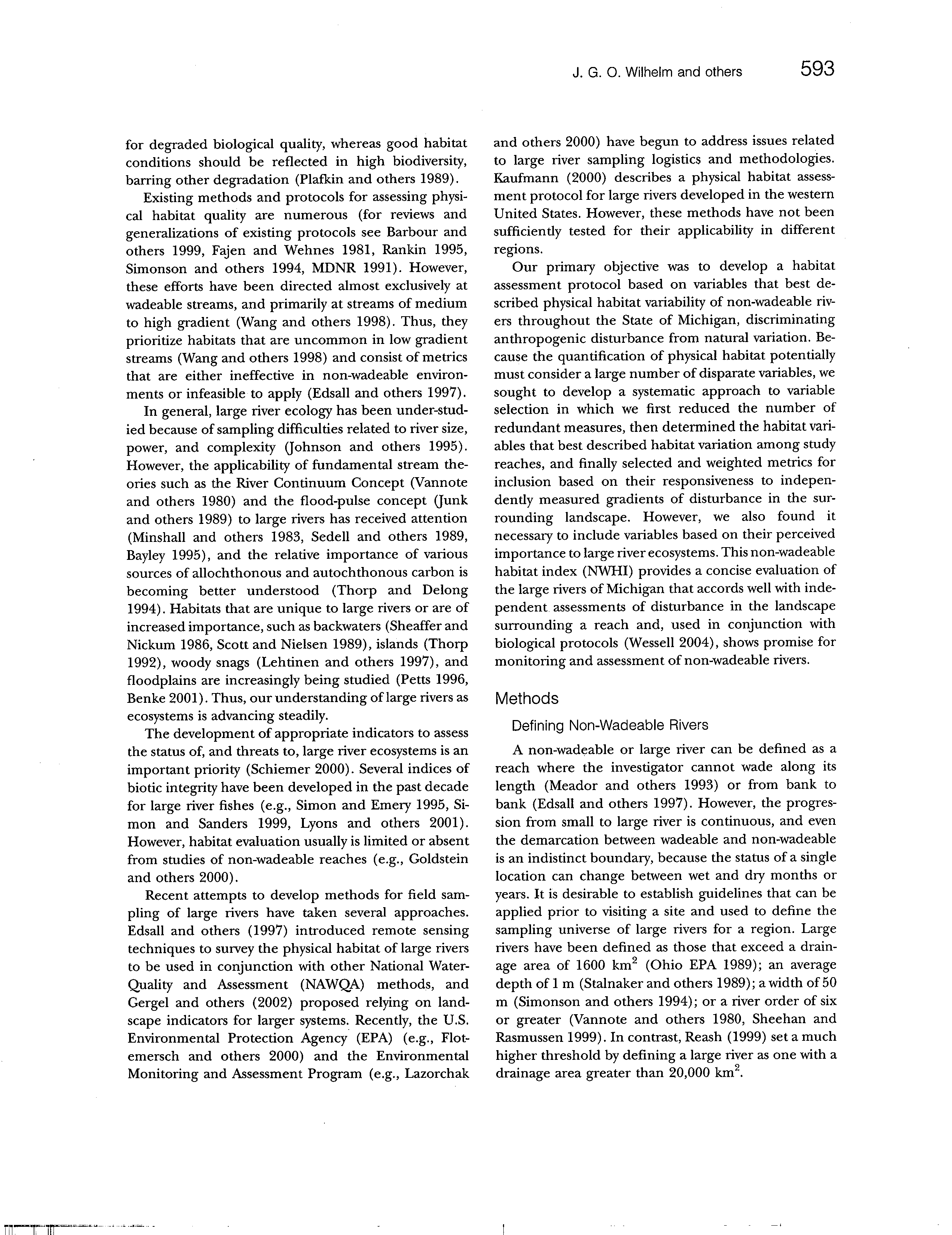
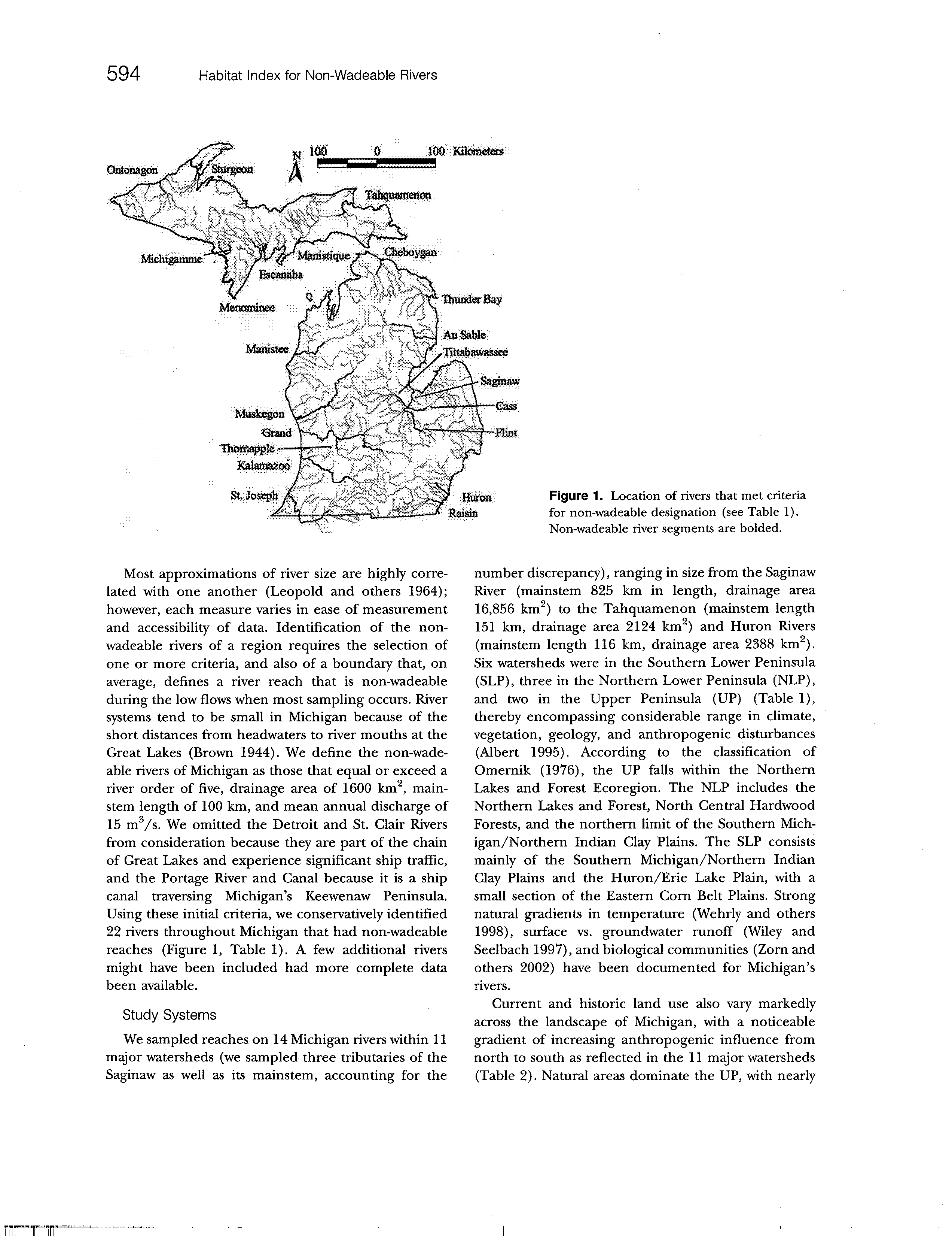
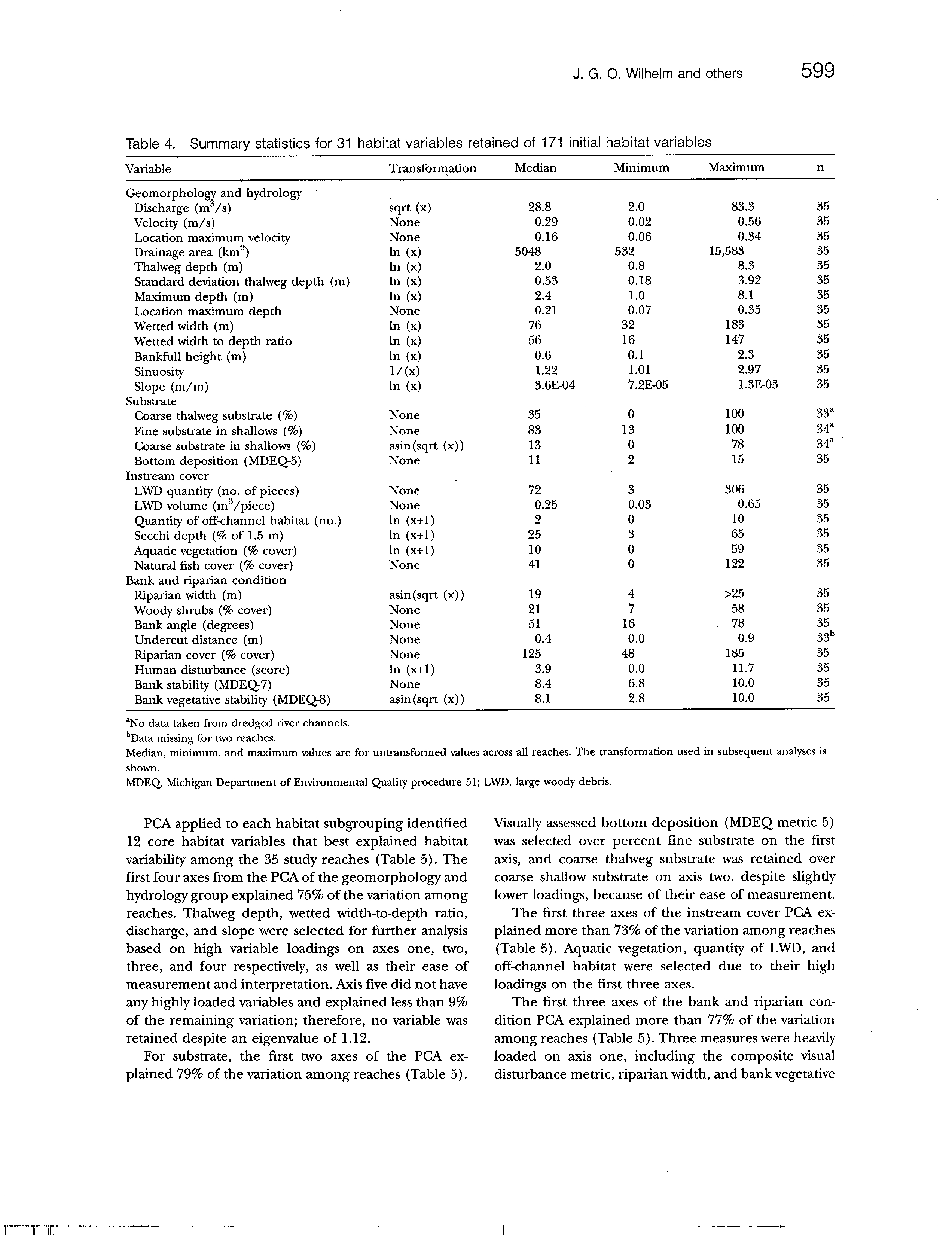
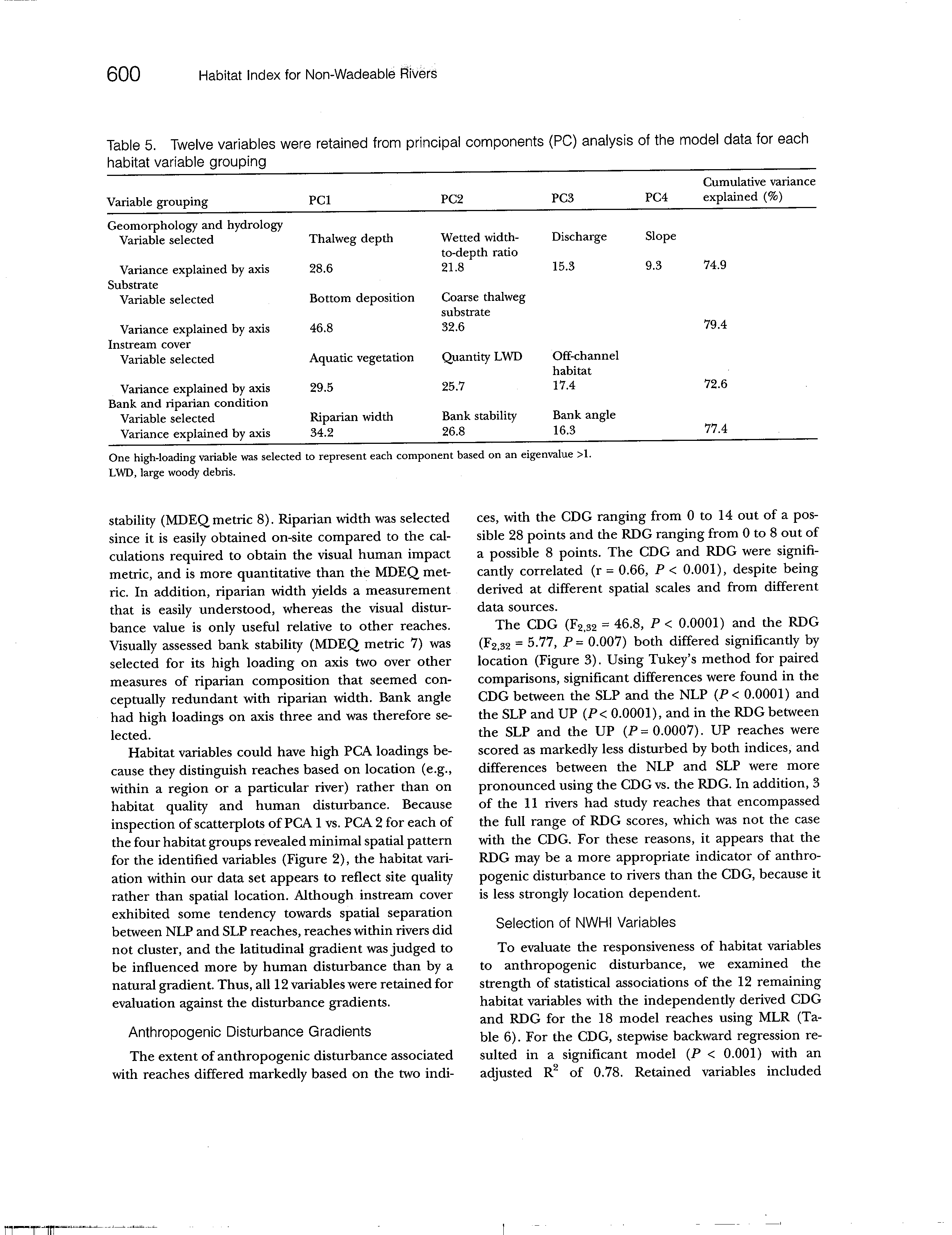
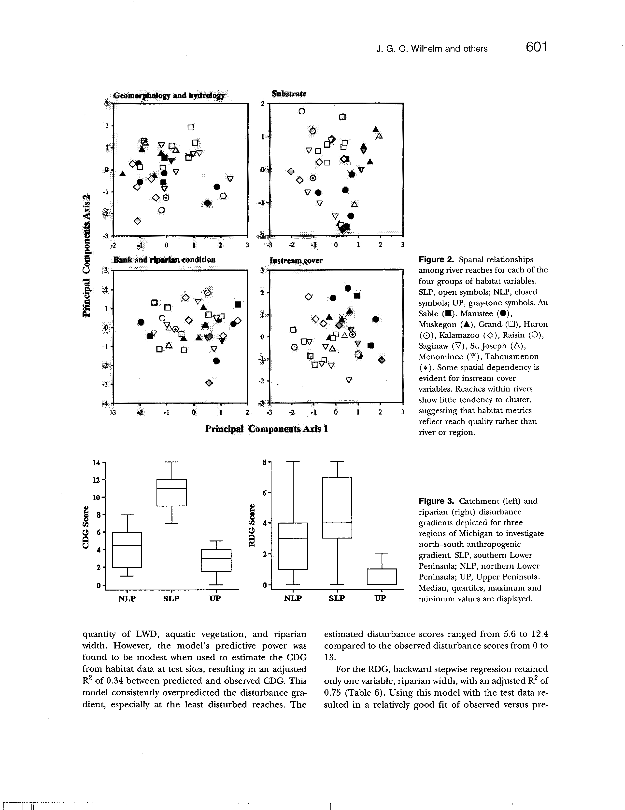
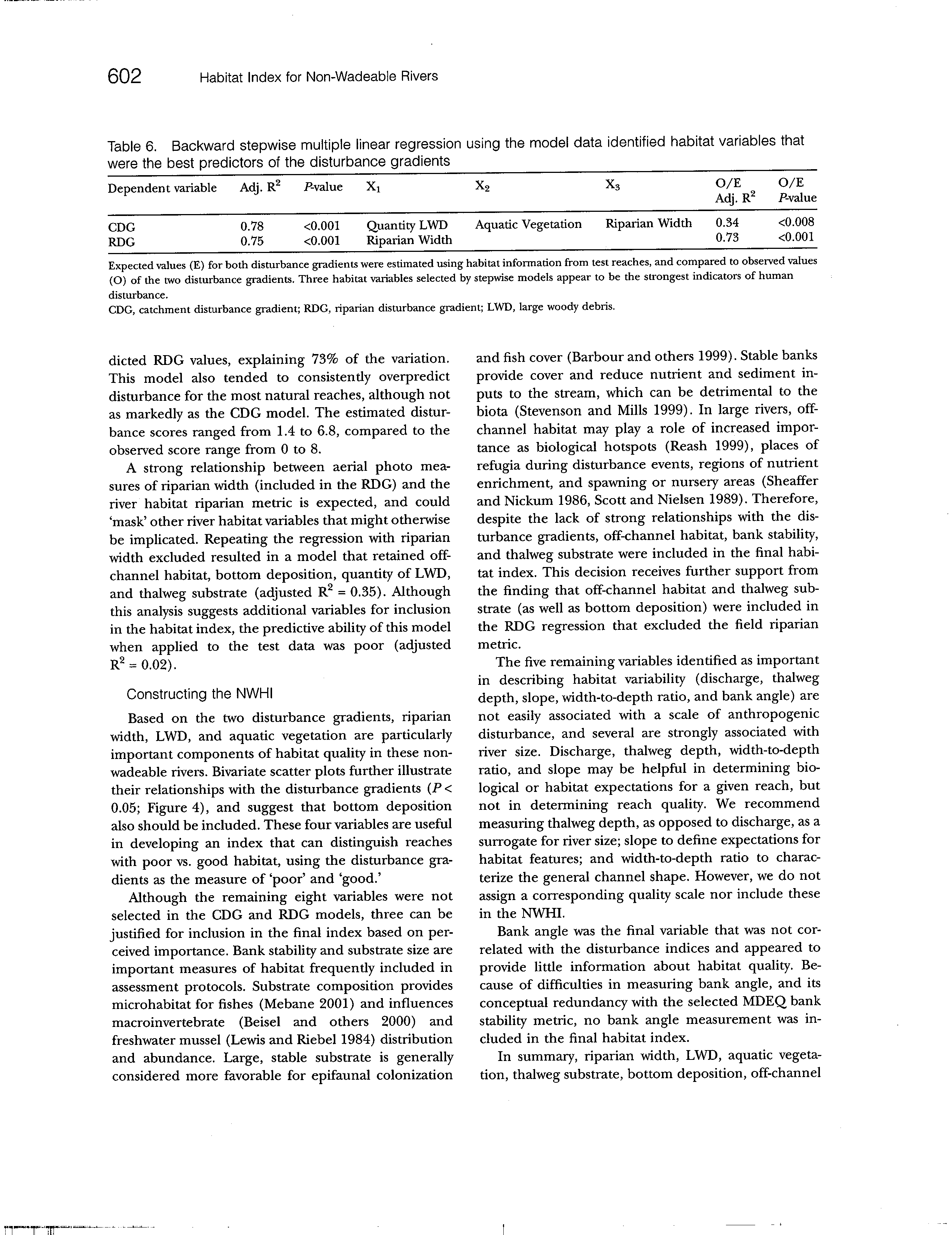
Wilhelm, J.G.O., Allan, J.D., Wessell, K.J., Merritt, R.W., and Cummins, K.W. 2005. Habitat

Assessment of Non-Wadeable Rivers in Michigan. Environmental Management Vol. 36,

No. 4, pp. 592-609.

Yoder, C.O. and Rankin E.T. 1998. The

Role of Biological Indicators in a State

Water Quality

Management Process. Environmental

Monitoring

and Assessment

,

Vol. 51, pp.

61-88.

19

---

---

Attac

h

ment

1

---

flabitat Strlntions N_>L

QUALIFICATIONS

Demonstrated management

abilities and leadership skills

Excellent concept generation

and synthesis skills - innovative

solutions to complex problems

Experience dealing with multiple

stakeholders and partners during

project planning and design

Strong facilitation and

communication skills

EXPERTISE

Conservation Geology

Aquatic Habitat Characterization

Nearshore Coastal Processes

Fluvial Sedimentology

Hydrology

Aquatic Invasive Species

Geospatial (GIS) Mapping

EDUCATION

B.S., Geology, Hobart College,

Geneva, New York, 1971

M.S., Geology, University of

Wisconsin, Madison, Wisconsin 1977

Ph.D., Sedimentology, State

University of New York, Binghamton,

New York, 1993

AFFILIATIONS

International

Association of Great

Lakes Research

Geological Society of America

American Water

Resources

Association

Wisconsin Wetlands Association

American Fisheries Society

American Shore

and Beach

Preservation Association

Dr. Mackey is Principal and Owner of Habitat Solutions NA, an environmental

consulting firm based in the Chicago, Illinois region. Habitat Solutions NA is an

environmental consulting firm specializing in aquatic habitat assessment, protection,

and restoration; riverine and coastal physical processes and habitat dynamics; and

Great Lakes water resource issues. Dr. Mackey holds a Doctorate in Geology (fluvial

sedimentology) with areas of technical specialization in aquatic habitat characterization

and mapping; development of biophysical linkages to habitat; surface and watershed

hydrology; nearshore, coastal, and riverine processes; and application of geospatial

data and analyses (GIS) to Great Lakes aquatic ecosystems.

Dr.

Mackey has considerable experience working with multiple stakeholders and has

been directly involved with policy development and numerous protection and

restoration initiatives focused on a broad range of environmental issues, including:

Great Lakes water resources and diversions (Annex 2001), aquatic invasive species

(ballast

water introductions and Asian Carp), natural flow regime restoration (dam

removals and watershed flow-path analyses), and the mapping and characterization of

fish and aquatic habitats in large riverine and nearshore systems of the Great Lakes.

He has collaborated with many key environmental groups and resource management

agencies in both the U.S. and Canada and has an excellent rapport with agency,

academic, and NGO organizations within the Great Lakes basin. Dr. Mackey has

strong facilitation

and communications skills and has considerable experience

developing innovative solutions to complex environmental problems within the Great

Lakes basin.

Dr.

Mackey served as Supervisor for the Lake Erie Geology Group for the Ohio

Department of Natural Resources and worked for the Great Lakes Governors as

Project Implementation Manager with the Great Lakes Protection Fund (GLPF). Dr.

Mackey developed, reviewed, and participated in numerous aquatic habitat protection

and restoration projects in both coastal and riverine settings. He currently holds a dual

appointment as an Adjunct and Visiting Research Professor in the Departments of

Biological Sciences and Earth Sciences at the University of Windsor, Canada.

RELEVANT

AGENCY EXPERIENCE

Dr. Mackey served as the Supervisor of the Lake Erie Geology Group from 1992 through 2003. This field office

provided technical support and services to lakefront property owners, local communities, and local, State, and

Federal agencies. The primary focus of this office was to develop a better understanding of coastal erosion and

sediment transport processes along the Ohio Lake Erie coastline, and how to manage those processes in a

sustainable

way that benefits the people of the State of Ohio. The Lake Erie Geology Group worked closely with the

U.S. Army Corps of Engineers on numerous coastal issues and assisted with the technical evaluation of projects

proposed for Ohio Lake Erie waters. This office reviewed applications for new shore protection projects as part of a

multi-agency review process, with a strong focus on sand resource conservation and management.

From 1992 though 1996, Dr. Mackey was a co-PI with the USGS National Coastal Center as part of major study to

document and understand the underlying framework and processes influencing coastal erosion

along

the Ohio Lake

Erie coastline. Dr.

Mackey also initiated a comprehensive inventory of shore protection structures and a

comprehensive assessment of the distribution of lakebed materials in coastal margin and nearshore zones in Ohio

waters.

Working with coastal stakeholders, the Lake Erie Geology Group developed and implemented the protocols

to systematically map and quantify Coastal Erosion Areas as part of the Ohio Coastal

Management

Program.

Dr. Mackey also initiated habitat-related projects in cooperation with both State and Federal agencies, with a specific

emphasis on developing linkages between physical habitat structure, the processes that create and maintain those

habitats, and the biological organisms that relay on those habitats. Examples include the Metzger Marsh wetland

restoration project, an assessment of Walleye spawning habitat over the Western Basin Reefs, mapping of potential

small-mouth bass habitat around the fringes of the Lake Erie Islands, and numerous dam removal and stream habitat

assessment and protection projects in tributaries flowing into Lake Erie.

Phone: (847) 360-9820 Cell: (224) 430-0813 Fax: (847) 625-0925 a-Mail: scudder@sdmackey.com

I

---

RELEVANT PROJECT

EXPERIENCE

TRCA - Toronto

Region Conservation

Authority -

Restoration and Naturalization

of Lower Don River,

Toronto, Ontario (

ongoing

) In cooperation with Staff from Applied Ecological Services and the Toronto Regional

Conservation Authority, Dr. Mackey is mapping channel morphology and potential fish habitat structure in three urban

rivers in the Greater Toronto area. Two of these rivers are being used as reference sites to establish habitat-fish

community relationships from areas that have not been severely degraded. It is anticipated that this information and

data will be used to guide a comprehensive restoration and naturalization effort in the Lower Don River.

The Ohio State University -

Aquatic Habitat Mapping and Assessment

-

Sandusky Bay and Sandusky River,

northern Ohio

(

ongoing

) In May 2008, Dr. Mackey working in collaboration with a Graduate Student from the OSU

Aquatic Ecology Laboratory and Fisheries Biologists from the ODNR mapped the distribution of aquatic and fish

habitats in the Sandusky River and Sandusky Bay using sidescan sonar. This ongoing work is supported by the

ODNR - Division of Wildlife. This study is part of an ongoing project to establish baseline data in anticipation of the

removal of Ballville Dam on the Sandusky River in Fremont, Ohio.

ODNR

-

Division of Wildlife

- Reconnaissance Sidescan Sonar Data Acquisition

-

Mentor/Fairport area

(ongoing

) In May 2008, Dr. Mackey working in collaboration with Fisheries Biologists from the ODNR - Division of

Wildlife, collected more than 50 line miles of sidescan sonar data from nearshore and offshore waters in Lake Erie as

part of a regional fish habitat characterization project. These data will be integrated with older data collected by the

ODNR - Division of Wildlife to develop linkages between fish communities and nearshore habitat distributions. These

data are being used to identify and guide potential fish habitat restoration and protection projects within Maumee Bay.

OMNR

- Lake

Erie Fisheries Management Unit - Lake Erie nearshore Mapping and

Lake Trout

Rehabilitation

(ongoing

) In July 2007, Dr. Mackey working in collaboration with Fisheries Biologists from the Ontario Ministry of

Natural Resources (OMNR), initiated a project to collect sidescan sonar data from nearshore areas of the Canadian

Lake Erie coastline to identify and characterize potential lake trout fish spawning habitat in the eastern basin of Lake

Erie.

The OMNR, USFWS, NYDEC, ODNR, and USGS are working to rehabilitate native lake trout populations in

Lake Erie through habitat protection and rehabilitation efforts combined with an intensive stocking effort to begin in

the fall of 2008. These habitat data will be used to locate potential stocking sites in both Canadian and U.S. Lake Erie

waters.

U.S. EPA

-

Nearshore and Coastal Margin Habitat Assessment Project (completed)

In cooperation with Michigan State University, Dr. Mackey was a co-PI on a project to characterize nearshore habitat

zones and develop biophysical linkages between nearshore habitats and the aquatic organisms that use them. Dr.

Mackey used sidescan sonar and underwater video to identify and map nearshore and coastal margin habitats off the

Lake Michigan coastlines of Wisconsin and northern Illinois. He continues to work with aquatic ecologists and fishery

biologists from Michigan State University to characterize the biophysical linkages and heterogeneity of nearshore

substrates.

Ultimately, the results of this work will be used to assess the potential impact of changing water levels

(climate change) and shoreline modifications (armoring) on nearshore habitat distribution and structure. The

Wisconsin DNR and Regional Planning Commissions will use this information to guide development of new rules for

shoreline development to protect and restore fish and aquatic habitats in Lake Michigan nearshore waters.

U.S. EPA - Lake

Erie Binational Map Project

(

completed)

In cooperation with the University of Minnesota, the University of Windsor, Great Lakes Commission, and the U.S.

Geological Survey, Dr. Mackey was a co-PI on a project to develop a unified habitat classification system and map for

the entire Lake Erie basin. This project developed tools to assist the Lake Erie Lakewide Management Plan (LaMP)

to develop a bi-national inventory of the status and trends in the quantity and quality of fish and wildlife habitats in the

Lake Erie basin. The integrated habitat map will be used to track improvements in habitat quantity and quality

resulting from preservation, conservation, and restoration efforts and to guard against further loss or degradation from

land-use alterations. The project team is developed a strategy to revise and expand the classification scheme to the

rest of the Lake Erie Basin and also developed a binational habitat map data exchange website which includes links

to geospatial metadata and habitat coverages in the basin. The Lake Erie habitat classification and mapping project

serves as a model for the development of a comprehensive basinwide habitat classification system and inventory for

the entire Great Lakes basin.

2

---

bit.1f Solutions S_1

ODNR

-

Division of Wildlife

-

Reconnaissance Sidescan Sonar Data Acquisition

-

Maumee Bay

(

completed)

In early May 2007, Dr. Mackey working in collaboration with Fisheries Biologists from the ODNR - Division of Wildlife,

collected more than 75

line miles

(121 line km) of sidescan sonar data from shallow-

water areas

of Maumee as part

of a regional fish habitat characterization project.

These data will be integrated with older data collected by the

ODNR - Division of Geological Survey that characterizes nearshore substrate distributions along the entire 262-mile

Lake Erie shoreline and more recent data collected by Environment Canada in deeper-

water areas

of the Western

Basin

.

These data are being used to identify and guide potential fish habitat restoration and protection projects within

Maumee Bay.

SEWRPC - Racine County Shore Structure Inventory and Assessment Project (completed)

In cooperation with the Southeast Wisconsin Regional Planning Commission and the Wisconsin DNR, Dr. Mackey

developed and implemented a set of field protocols to identify, characterize, map, and inventory shore protection

structures along the Racine County Lake Michigan shoreline. This pilot project included extensive field work and data

collection using portable GPS equipment and development of a geospatial database and GIS to assess the current

state of shoreline armoring along the Wisconsin Lake Michigan shoreline. As part of this project, the condition and

integrity of structures were assessed along with the potential of these structures to modify nearshore coastal

processes and habitats. In part based on this work and a similar inventory of shore protection structures along

Wisconsin Lake Michigan shoreline, Dr. Mackey recently developed a new shoreline

alteration

index (SAI) that

assesses

not only the physical impacts of shore protection in the nearshore zone, but potential biological impacts as

well.

Ultimately, the results of this work will be combined with results from the U.S. EPA project (described above) to

assess the impact of shoreline armoring on coastal processes and nearshore habitat distribution and structure.

USFWS

-

Restoration Act Sponsored Research

(

completed)

In cooperation with the University of Windsor and The Ohio State University, Dr. Mackey was a co-PI on a recently

completed project designed to create a framework and develop a process to systematically identify, coordinate, and

implement aquatic and fish habitat restoration opportunities in the Lake Huron to Lake Erie Corridor (Huron-Erie

Corridor, HEC) within a context of water-level change resulting from potential long-term effects of global climate

change.

This project summarized existing datasets and initiatives and developed a comprehensive strategy to

identify and implement sustainable aquatic and fish habitat restoration opportunities within the Corridor. Components

of this restoration strategy are currently being implemented by the U.S. Geological Survey, U.S. Fish & Wildlife

Service, Michigan DNR, Environment Canada, and the Great Lakes Commission.

International Joint Commission

-

Great Lakes Water Quality Agreement

(

completed)

In 2005, the Water Quality Board of the International Joint Commission retained Dr. Mackey to explore more fully the

role of physical integrity as part of a comprehensive ongoing review of the Great Lakes Water Quality Agreement.

Currently the GLWQA is a "water chemistry" agreement that does not adequately define or incorporate the critical

elements of physical or biological integrity.

Dr.

Mackey's work succinctly defined physical integrity and provides

specific examples of the importance of physical integrity to both the environmental and economic health of the Great

Lakes basin.

This work provides the conceptual underpinnings for a suite of developing projects focused on the

protection and restoration of fish and aquatic habitats within connecting channels and waters (St. Clair and Detroit

Rivers) and Lake St. Clair. Moreover, this work may form the basis for delisting criteria for Benthic Habitat and Fish

and Wildlife populations within the St. Clair and Detroit River AOCs. Incorporating physical integrity into the GLWQA

will

provide new policy guidance and broaden the scope of the Agreement to include heretofore unrecognized

protection and restoration opportunities within the Great Lakes basin.

SERVICE

Dr.

Mackey currently serves as a member

of Lake Erie Habitat Task Group for the Great Lakes Fisheries

Commission

and the

AIS Barrier Advisory Panel and Rapid Response Team

for the USACE Chicago Waterway

electric field barrier project.

3

I

---

Habitat SoTutiow I

HONORS

/

AWARDS

Letters of Commendation

-

Ohio Senate

,

U.S. House of Representatives

,

Spring 2001

: For services to the

People of the State of Ohio and the Natural Resources of Lake Erie.

Speaker

,

Plenary Session

-

International Association for Great Lakes Research

,

1999

:

Cumulative Impacts:

Physical and Biological Linkages to Habitat.

42"d Conference on Great Lakes Research, Cleveland, Ohio, May 24-28.

Outstanding Paper

-

Journal of Sedimentary Research

,

1995

:

Three-dimensional model of alluvial stratigraphy:

theory and application.

Award conferred at SEPM President's Reception, 1997, Society Records and Activities,

Journal of Sedimentary Research, v. 67, no. 6, p. 1103-1114.

SELECTED PUBLICATIONS

Mackey, S.D.,

in review,

Climate Change Impacts and Adaptation Strategies for Great Lakes Nearshore and Coastal

Systems:

Climate

Change

in

Great Lakes

Region - Decision Making Under Uncertainty,

Michigan State

University, East Lansing, Michigan. (invited)

Mackey, S.D. and R.R. Goforth, 2005, Great Lakes Nearshore Habitat Science:

in

Mackey, S.D. and R.R. Goforth,

eds. Great Lakes nearshore and coastal habitats: Special Issue, Journal of Great Lakes Research 31

(Supplement 1), p. 1-5.

Mackey, S.D. and D.L. Liebenthal, 2005, Mapping changes in Great Lakes nearshore substrate distributions:

in

Mackey, S.D. and R.R. Goforth, eds. Great Lakes nearshore and coastal habitats: Special Issue, Journal of Great

Lakes Research 31 (Supplement 1), p. 75-89.

Meadows, G.A., Mackey, S.D., Goforth, R.R., Mickelson, D.M., Edil, T.B., Fuller, J., Guy, D.E. Jr., Meadows, L.A.,

Brown, E., Carman, S.M., and Liebenthal, D.L., 2005, Cumulative Impacts of Nearshore Engineering:

in

Mackey,

S.D. and R.R. Goforth, eds. Great Lakes nearshore and coastal habitats: Special Issue, Journal of Great Lakes

Research 31 (Supplement 1), p. 90-112.

Mackey, S.D.,

in press,

Lake Erie Sedimentation and Coastal Processes: in Ciborowski, J.J.H., M.N. Charlton, R.G.,

Kreis, Jr., and J.P. Reutter (ed), Lake Erie at the millennium - changes, trends, and trajectories. Canadian

Scholars' Press Inc, Toronto, ON. (invited)

Evans, J. E., Mackey, S. D., Gottgens, J. F. and Gill, W. M., 2000, From Reservoir to Wetland: The Rise and Fall of an

Ohio Dam: in Schneiderman, J.L. (ed), The Earth around us: Maintaining a livable planet:

W.H. Freeman Co.,

San Francisco, CA. p. 256-267. (invited)

Evans, J.E., Mackey, S.D., Gottgens, J.F., and Gill, W.M., 2000, Lessons from a Dam Failure: Ohio Journal of

Science, v. 100, no. 5, p. 121-131.

Evans, J.E., Gottgens, J.F., Gill, W.M., and Mackey, S.D., 2000, Sediment Yields controlled by Intrabasinal Storage

and Sediment Conveyance over the Interval 1842-1994: Chagrin River, Northeast Ohio, U.S.A.: Journal of Soil

and Water Conservation, v. 55, no. 3, p. 264-270.

Roseman, E.F., Taylor, W.B., Hayes, D.B., Haas, R.C., Davies, D.H., and Mackey, S.D., 1999, Influence of Physical

Processes on the early life history stages of Walleye,

Stizostedion vitreum,

in western Lake Erie: Ecosystem

Approaches for Fisheries Management, University of Alaska Sea Grant Program, AK-SG-99-01.

Berkman, P.A., Haltuch, M.A., Tichich, E., P.A., Garton, D.W., Kennedy, G.W., Gannon, J.E., Mackey, S.D., Fuller,

J.A., and Liebenthal, D.L., 1998, Zebra mussels invade Lake Erie muds: Nature, v. 393, p. 27-28.

Mackey, S.D. and Bridge, J.S., 1995, Three-dimensional model of alluvial stratigraphy: theory and application,

Journal of Sedimentary Research, v. B65, no. 1, p. 7-31.

Bridge, J.S., and Mackey, S.D., 1993, A theoretical study of fluvial sandstone body dimensions, in: Flint, S. and

Bryant, I.D. (ed), The Geological Modeling of hydrocarbon Reservoirs and Outcrop Analogues, International

Association of Sedimentologists Special Publication No. 15, p. 213-236.

Bridge, J.S., and Mackey, S.D., 1993, A revised alluvial stratigraphy model, in: Marzo, M. and Puigdefabregas, C.

(ed), Alluvial Sedimentation, International Association of Sedimentologists Special Publication No. 17, p. 319-336.

Mackey, S.D. and Bridge, J.S., 1992, A revised FORTRAN program to simulate alluvial stratigraphy: Computers and

Geosciences, v. 18, no. 3, p. 119-181.

4

I

---

habitat

Solutions \.

TECHNICAL REPORTS

Mackey

,

S.D., 2006

,

Great Lakes

Dry

Cargo

Sweepings Impact Analysis

-

Sidescan

Sonar

Data Acquisition:

Final

Report

,

USDOT Volpe Transportation Center and U.S. Coast Guard

,

Washington

,

D.C. 48 p. plus appendices.

Mackey

,

S.D., Reutter

,

J.M, Ciborowski

,

J.J.H., Haas

,

R.C., Charlton

,

M.N., and Kreis

,

R.J., 2006,

Huron-Erie

Corridor system Habitat

Assessment

-

Changing Water levels and Effects of Global Climate Change

:

Project

Completion Report

,

USFWS Restoration Act Sponsored Research Agreement #30181-4

-

J259. 47 p.

Mackey

,

S.D., Johnson

,

L.B., Ciborowski, J.J.H., Hollenhorst

,

T., 2006,

Planning for an Integrated Habitat

Classification System

and Map for the

Lake

Erie Basin

:

Summary Report

-

Workshop II, University of Windsor,

Windsor

,

ON. January 2006. 33 p.

Mackey

,

S.D. 2005

,

Assessment

of Lake Michigan Shoreline Erosion Control Structures in Racine County.

Southeast

Wisconsin Regional Planning Commission

,

Waukesha

,

WI. 36 p.

Mackey

,

S.D., 2005

,

Physical Integrity of the Great

Lakes

:

Opportunities for Ecosystem Restoration

:

Report to the

Great Lakes Water Quality Board

,

International Joint Commission,

Windsor, ON.

Mackey

,

S.D. and Bridge

,

J. S., 1990

,

The

use of

empirical data to predict alluvial channel-belt geometry

:

a critical

evaluation

:

SUNY technical report, 22 p.

USGS OPEN

-

FILE REPORTS

/

TECHNICAL REPORTS

Mackey

,

S.D., 1996

,

Multivariate recession factor analysis

-

Ashtabula and Lake Counties

,

Ohio, in

:

Folger, D.W.

(ed), Lake Erie Coastal Erosion Study Workshop

-

August 1996

:

USGS Open

-

File Report 96-507.

Mackey, S.D., 1996

,

Relationship between sediment supply

,

barrier systems

,

and wetland loss in the western basin

of Lake Erie

-

a conceptual model, in

:

Folger

,

D.W. (ed), Lake Erie Coastal Erosion Study Workshop - August

1996

:

USGS Open-File Report 96-507.

Mackey

,

S.D., 1995

,

Lake Erie Wetlands

-

Metzger Marsh Restoration Project, in: Folger

,

D.W. (ed

),

Lake Erie

Coastal Erosion Study Workshop

-

April 1995

:

USGS Open-File Report 95-224.

Mackey

,

S.D., 1995

,

Lake Erie Sediment Budget, in: Folger, D.W. (ed

),

Lake Erie Coastal Erosion Study Workshop -

April 1995

:

USGS Open

-

File Report 95-224

,

p. 34-37.

Mackey

,

S.D. and Guy

,

D.E., Jr

.,

1994, Geologic framework and restoration of an eroded Lake Erie coastal marsh -

Metzger Marsh

,

Ohio, in

:

Folger, D.W. (ed

),

Lake Erie Coastal Erosion Study Workshop - February 1994: USGS

Open

-

File Report 94

-

200, p. 28-31.

Mackey, S.D. and Guy

,

D.E., Jr

.,

1994

,

Comparison of long

-

and short

-

term recession rates along Ohio's Central

Basin shore of Lake Erie, in: Folger

,

D.W. (ed

),

Lake Erie Coastal Erosion Study Workshop

-

February 1994:

USGS Open-File Report 94

-

200, p

. 19-27.

ABSTRACTS/

PRESENTATIONS

Mackey

,

S.D., 2007

,

Lakebed Erosion of Cohesive Clays -An Alternative Erosion Hypothesis: International

Association for Great Lakes Research

,

50th Conference on Great Lakes Research, State College, Pennsylvania,

May 28

-

June 1, 2007.

Gerke

,

B., Livchak

,

C., and Mackey, S.D., 2007, A New Indicator of Shoreline Alteration for Lake Erie: International

Association for Great Lakes Research

,

50th Conference on Great Lakes Research, State College

,

Pennsylvania,

May 28

-

June

1, 2007.

Mackey

,

S.D., 2007

,

Climate Change Impacts and Adaptation Strategies for Great Lakes Nearshore and Coastal

Systems

:

Climate Change in

Great Lakes

Region

-

Decision Making Under Uncertainty

,

Michigan State

University

,

East Lansing

,

Michigan

,

March 15-16, 2007

(

invited)

Mackey, S.D. 2006

,

A Natural History of the Great Lakes

-

How Landscapes and Processes Create an Ecosystem:

National Estuarine Research Reserves Annual Meeting

,

Huron

,

Ohio. October 16, 2006.

Mackey

,

S.D., Brammeier

,

J. and Polls

,

I., 2006

,

The Case for Ecological Separation of the Mississippi River and the

Great Lakes Basins via the Chicago Waterway System

:

International Association for Great Lakes Research, 49th

Conference on Great Lakes Research

,

Windsor

,

Ontario

.

May 22

-

26, 2006.

5

---

habitat

solufiaw NA

Mackey, S.D., 2005, Physical Integrity - Linking Landscapes to the Lakes:

2005 A.D. Latornell Conservation

Symposium,

Alliston, Ontario, November 16-18, 2005. (invited)

Mackey

,

S.D. and Goforth, R.R., 2005

,

Lake Michigan Nearshore Habitat, Protection

,

and Restoration

:

Lake Michigan

State o the

Lake

Conference,

Green Bay, Wisconsin, November 2-3, 2005. (invited)

Mackey, S.D. and Hahn, M.G., 2005, Inventory and Assessment of Lake Michigan Shoreline Erosion Control

Structures in Racine County: Lake

Michigan

State

of the Lake Conference,

Green Bay, Wisconsin, November 2-3,

2005. (invited)

Mackey, S.D., Ciborowski, J.J.H. and Haas, 2005, Things to Consider- Habitat Dynamics and Changing Water Level

Regimes

:

Lake St. Clair Biennial Conference

,

Wallaceburg

,

Ontario, September 21-22. (invited)

Mackey, S.D., 2004, Wetland Hydrology, Connectivity, and Water

Balance

:

Constructed Wetlands Workshop,

Lake

Erie Center, University of Toledo, Toledo, Ohio, June 16-18, 2004. (invited)

Mackey

,

S.D., 2004

,

A Conceptual Framework for Nearshore and Coastal Habitats

:

International Association for

Great Lakes Research, 47th Conference on Great Lakes Research, Waterloo, Ontario

,

May 24-28, p. 95. (invited)

Meadows, G.A., Mackey, S.D. Mickelson, D.M., Edil, T.B., Goforth R., Guy Jr., D.E., and Fuller, J.A., 2004,

Cumulative Habitat Impacts of Nearshore Engineering

:

International Association for Great Lakes Research, 47tt

Conference on Great Lakes Research, Waterloo, Ontario, May 24-28, p. 105. (invited)

Tyson

,

J.T., Ryan

,

P.A., and Mackey

,

S.D., 2004

,

Nearshore Habitat in Lake Erie: Physical Habitat and Biological

Accommodation at Relevant Spatial Scales

:

International Association for Great Lakes Research, 47th Conference

on Great Lakes Research

,

Waterloo

,

Ontario, May 24

-

28, p. 157

. (

invited)

Mackey

,

S.D., 2004

,

Coastal Erosion Processes

:

Erosion Mechanics and Models

:

Coastal

Bluff and Dune Erosion

Forum and Workshop,

Sheboygan River Partnership, University of Wisconsin Extension, Wisconsin Coastal

Management Program

,

University of Wisconsin

-

Sheboygan

,

Sheboygan

,

Wisconsin

,

March 20

,

2004. (invited)

Mackey

,

S.D., 2003

,

Changing Water Levels in Lake Erie and Linkages to Ecosystem Health

:

International

Association for Great Lakes Research

,

46th Conference on Great Lakes Research, Chicago, Illinois, June 23-26,

p.124. (invited)

Mackey, S.D., 2003, A Conceptual Framework for Nearshore and Coastal Habitats:

Research,

Assessment,

and Data

Needs

to Promote protection

of Great Lakes

Nearshore Fisheries Habitat Workshop,

Michigan Natural Features

Inventory and the Great Lakes Fishery Trust, April 1-2, 2003, Muskegon, Michigan. (invited)

Mackey, S.D., Liebenthal, D.L., and Fuller, J.A., 2003, Nearshore Habitat Dynamics: Research, Assessment, and

Data

Needs

to Promote protection of Great

Lakes Nearshore

Fisheries Habitat Workshop,

Michigan Natural

Features Inventory and the Great Lakes Fishery Trust, April 1-2, 2003, Muskegon, Michigan. (invited)

Mackey

,

S.D., 2003

,

Hydrology and fish habitat issues in the St. Clair Delta

:

Annual Meeting, Lake Erie Committee -

Great Lakes Fishery Commission

,

March 24

-

25, 2003

,

Port Huron

,

Michigan

. (

invited)

Mackey, S.D., 2003, Great Lakes Coastal Margins:

2"d Habitat Protection and Restoration Workshop,

Lake Erie

Millennium Network, February 11-13, 2003, Windsor, Ontario. (invited)

Mackey, S.D., 2002, Great Lakes Nearshore Coastal Habitats:

1St

Habitat Protection and Restoration Workshop,

Lake

Erie Millennium Network

,

December 9-10, 2002

,

Windsor, Ontario

. (

invited)

Mickelson

,

D.M., Brown

,

E.A., Edil, T.B., Meadows

,

G.A., Mackey, S.D., Liebenthal, D.L., and Fuller

,

J.A., 2002,

Comparison of sediment budgets of bluff/beach/nearshore environments near Two Rivers

,

Wisconsin

,

on Lake

Michigan

,

and at Painesville

,

Ohio, on Lake Erie: Geological Society of America Abstracts with Programs, v. 34,

no. 2, p. A-12.

Mackey

,

S.D., Foye

,

D.A., Davies

,

D.H., and S

.

Wells, 2001

,

Structural Habitat

:

Substrate and morphology in Riverine

Environments

:

International Association for Great Lakes Research

, 44th

Conference on Great Lakes Research,

Green Bay, Wisconsin, June 10-14, p. 79.

Fuller, J.A., Liebenthal

,

D. L., and Mackey

,

S.D., 2001

,

The use of sidescan sonar to map sediment distribution and

track littoral transport in Lake Michigan and Lake Erie: International Association for Great Lakes Research, 44th

Conference on Great Lakes Research

,

Green Bay

,

Wisconsin

,

June 10

-

14, p. 44.

Liebenthal

,

D.L., Fuller

,

J.A., and Mackey

,

S.D., 2001

,

Application of Sidescan Sonar and GIS Technologies to Map

Nearshore Sand Distribution in Lake Michigan and Lake Erie

:

International Association for Great Lakes Research,

44th Conference on Great Lakes Research, Green Bay, Wisconsin, June 10-14, p. 75.

Carman, S.M., Goforth, R.R., Meadows, G.A., and Mackey, S.D., 2001, Associations between Great Lakes

Nearshore Communities and Habitats Influenced by Varied Levels of Shoreline Development

:

International

Association for Great Lakes Research

,

44th Conference on Great Lakes Research

,

Green Bay

,

Wisconsin, June

10-14, p. 14.

6

I

---

Habitat Solutions NA

Graber,

B.E., Bowman

,

M., Carney, R.S., Doyle, M.W., Fisher, M., Mackey, S.D., and Wildman, L., 2001, Technical

Issues in Small

Dam Removal

Engineering

:

The Future of Dams and Their Reservoirs, United Sates Society on

Dams, 21st USSD Annual

Meeting and

Lecture Proceedings, Denver, CO.

Goforth, R.R., Meadows, G.A., and Mackey, S.D., 2001, Nearshore ecological properties associated with shoreline

processes in selected Great Lakes ecosystems: Coastal Zone '01 Conference, Cleveland, Ohio. (invited)

Goforth, R.R., Meadows, G.A., Mickelson, D.M., Edil, T.B., and Mackey, S.D., 2000, Associations between bluff

erosion processes and nearshore aquatic ecosystem properties along Great Lakes shorelines: Ecological Society

of America, Annual Meeting, Snowbird, Utah.

Mickelson, D.M., Brown, E.A. Edil, T.B., Meadows, G.A., Mackey, S.D., Liebenthal, D.L. and Fuller, J.A., 2000, An

integrated bluff-beach-nearshore sediment study in northeastern Wisconsin: Geological Society of America, 2000

Abstracts with Programs v. 32, no. 4 p. A-52.

Mackey, S.D., Guy, D.E., Meadows, G.E., Perlin, M., Ozkan-Haller, T., Mickelson, D.M., and Edil, T., 1999,

Nearshore models: A method to assess cumulative impacts of shoreline armoring on nearshore habitat:

Geological Society of America, North-Central Annual Meeting, Champaign-Urbana, Illinois, April 22-23, p. A-57.

Guy, D.E. and Mackey, S.D., 1999, Geologic studies along the Ohio shore of Lake Erie -1838 to 1999: Geological

Society of America, North-Central Annual

Meeting

,

Champaign-Urbana, Illinois, April 22-23, p. A-18.

Mackey, S.D. and Tyson, J.T., 1999, Identification and delineation of EcoZones based on physical characteristics of

structural habitat: International Association for Great Lakes Research, 42nd Conference on Great Lakes Research,

Cleveland, Ohio, May 24-28, p. A-75-A76.

Mackey, S.D., Foye, S.A., and Guy, D.L., Jr., 1999, Impacts and mitigation of the April 9, 1998 storm: Ohio's Western

Basin coastal area

: International Association for Great Lakes Research, 42nd Conference on Great Lakes

Research, Cleveland, Ohio, May 24-28, p. A-75.

Fuller, J.A., Mackey, S.D., and Liebenthal, D. L., 1999, Mapping and distribution of substrates from six Western Basin

reefs in Lake Erie: an update: International Association for Great Lakes Research, 42"d Conference on Great

Lakes Research, Cleveland, Ohio, May 24-28, p. A-35.

Mackey, S.D., 1999, Opportunities for Dam Removal and Riparian Habitat Restoration - Chagrin Falls, Ohio: Midwest

Fish and Wildlife Conference, Chicago, Illinois.

Mackey, S.D., Davies, D.H., Foye, D.A., 1999, Potential Physical and Biological Impacts of Dam Removal -

Sandusky River, Northwest Ohio: Midwest Fish and Wildlife Conference, Chicago, Illinois.

Mackey, S.D., and Dye, B.P., 1998, GIS Applications For Wetland Restoration

, Management

,

And Monitoring -

Metzger Marsh

, Lucas County, Ohio: Midwest/Great lakes ESRI-GIS Users Conference & Cincinnati Area GIS

(CAGIS) Technology Exposition, Cincinnati, Ohio.

Mackey, S.D. and Haines, J.W., 1998, Geological factors controlling recession - Ohio Lake Erie Coastline:

Geological Society of America, North Central Annual Meeting, Columbus, Ohio, v. 30, no. 2, p. 58

Mackey, S.D. and Foye, D.A., 1998, Relationship between sediment supply, barrier systems, and wetland loss in the

Western Basin of Lake Erie - a conceptual model: Geological Society of America, North Central Annual Meeting,

Columbus, Ohio, v. 30, no.2, p. 58

Dean, S.L., Drescher, E.W., Lime, J., VanArsdalen, R., Fuller, J.A., Liebenthal, D.L., and Mackey, S.D., 1998, Joint

pattern control on geomorphology of Lake Erie islands, Northern Ohio, U.S.A., in: Proceedings Woodworth

Conference on Fractures, University of Ulster, Coleraine Northern Ireland, p. 14

Mackey, S.D. and Davies, D.H., 1996, Identification, protection, and rehabilitation of fisheries habitat in riverine and

coastal

systems - a geological approach: American Fisheries Society Annual Meeting, Ann Arbor, Michigan.

(invited)

Guy, D.E., Jr., Fuller, J.A., and Mackey, S.D., 1994, Coastal response to breakwater construction at Geneva State

Park, Northeast Ohio: Geological Society of America, North Central Annual

Meeting

, Kalamazoo, Michigan, v. 26,

no. 5, p. 18.

Mackey, S.D., and Guy, D.E., Jr., 1994, A different approach to mapping coastal recession - combining the old with

the new: Geological Society of America, North Central Annual

Meeting

, Kalamazoo, Michigan, v. 26, no. 5, p. 52

Mackey, S.D., and Guy, D.E., Jr., 1994, Geologic framework of an eroded Lake Erie coastal marsh -- Metzger Marsh,

Ohio: Geological Society of America, North Central Annual Meeting, Kalamazoo, Michigan, v. 26, no. 5, p. 52

Lime, J.C., VanArsdalen, R.C., Dean, S., Mackey, S.D., Fuller, J.A., and Liebenthal, D.L., 1994, Fracture patterns,

shoreline and lake bottom features, Kelley's Island and South Bass

Island

, Lake Erie, Ohio: Geological Society of

America, North Central

Annual Meeting

, Kalamazoo, Michigan, v. 26, no. 5, p. 50.

7

---

Ttabitnt

Sdutions NA

Stone, B.D., Pavey

,

R.R., Guy

,

D.E., Jr

.,

and Mackey

,

S.D., 1993

,

Stratigraphy and erosion processes that control

Lake Erie bluff morphology

,

northeastern Ohio: International Association of Great Lakes Research, 36th

Conference on Great Lakes Research

,

De Pere

,

Wisconsin, June 4-10, p. 54.

Mackey

,

S.D. and Bridge

,

J.S., 1992

,

The use of a three-dimensional alluvial stratigraphy model to simulate the

effects of base

-

level change on alluvial deposition: Mesozoic of the Western Interior

,

sedimentological responses

to base level change

:

SEPM Rocky Mountain Section Meeting

,

August 1992.

Mackey

,

S.D. and Bridge

,

J.S., 1991, Alluvial stratigraphy models

-

a progress report

:

characterization of fluvial and

aeolian Reservoirs

:

Geological Society

,

University of Aberdeen

,

March 1991.

Bridge

,

J.S. and Mackey

,

S.D., 1989

,

Quantitative modeling of alluvial stratigraphy

:

a new look: Quantitative Dynamic

Stratigraphy

,

28th International Geological Congress, Washington

,

D.C., July 1989.

8

---

Attac

h

me

n

t 2

---

Scudder Mackey Attachment 2

Physical Characteristics of Aquatic Habitat

Climate

(Energy)

Habitat

Substrate

Water Mass

(Geology

)

(Hydrology)

•

Energy -

estimated from hydraulic

calculations for both oscillatory and

unidirectional flows

,

flow regime

•

Substrate -

bedrock

,

composition,

texture

,

hardness, stability,

porosity

,

permeability

,

roughness,

contaminants

,

macrophyte/woody

debris.

• Water

Mass

-

depth, temperature,

turbidity

,

nutrients

,

contaminants,

dissolved oxygen

,

and water

quantity.

•

Habitat -

physical characteristics

and energy conditions that meet

the needs of a specific species

and/or biological community for a

given life stage.

Figure 1. Fundamental Characteristics of Aquatic Habitat

---

A

tt

ac

hm

e

nt 3

---

Mackey Attachment 3

Table 1.

Data

Availability,

Metrics and Methods

Rankin

(

2004

),

CAWS IJAA

,

Habitat Evaluation and

Assessment Factor

Applicability

Statement of Reasons

Improvement Study

Number of Instream

Natural

and artificial

20 sampling sites based on

30 sampling sites based on

Sampling Sites

systems

availability offish data

,

no

consideration of physical

consideration of physical

habitat

,

geospatially integrated

habitat

with continuous monitoring

stations and shoreline/ bank-

edge inventory and assessment

Distance between

Natural and artificial

Min: 0.5 miles

(

0.8 km

)

Min: 0.25 miles

(

0.4 km)

Sampling Sites

systems

Max: 15

.

8 miles (25.4 km

)

Max: 9.6 miles

(15.3 km)

Mean

:

4.3 miles (6.9 km

)

Mean

:

2.9 miles

(4.7 km)

Continuous shoreline/bank-edge

inventory and

assessment

Type and Extent

of

Natural and artificial

Numerous sediment samples

Geospatial integration of

Substrates

systems

available -

not

used

in Aquatic

historic and new sediment

Life Use designation Analyses

sampling data

Substrate

Quality

Natural and artificial

Sediment chemistry and

Review and evaluation of

systems

contaminant data available -

not sediment quality data

,

including

used

in Aquatic Life Use

organic and inorganic chemical

designation Analyses

data

,

as well as sediment

toxicity data

;

geospatial

referencing

of historic

sediment

chemistry and contaminant data

Type and Extent

of

Natural and artificial

Data at 20 sampling sites, sites

Data at 30 sampling sites, sites

Instream Habitat Cover

systems

located based on available

located based on physical

fisheries data

habitat characteristics

Type and Extent

of

Natural and artificial

Unknown

,

not surveyed or

Geospatially referenced,

Shoreline and Bank-

systems

inventoried

.

Qualitative

continuous digital shoreline

Edge Habitats

observations only.

video for both banks of the

entire CAWS, for inventory and

assessment

Type

and Extent

of

Natural and artificial

Unknown

,

not surveyed or

Geospatially

referenced,

Riparian Cover

systems

inventoried

.

Qualitative

continuous digital shoreline

observations only.

video for both banks of the

entire CAWS,

for inventory and

assessment

Flow Regime and Water

N/A to CAWS as

Flow, water level, and hydraulic

Flow, water level, and hydraulic

Levels

flows and water

modeling data available - not

modeling data available, potential

levels are regulated

used in Aquatic Life Use

for analysis of conveyance,

for flood control,

designation

navigation impacts of proposed

conveyance of

restoration activities

wastewater,

navigation

Water

Quality

Natural and artificial

Complete suite of water quality

Rigorous evaluation of

systems

data available -

no evidence

continuous DO data,

that proposed increase in DO

supplemented with the DO

will yield significant biological

profiles conducted at the 29

response

habitat sampling stations

surveyed during 2008 season;

analysis of other water quality

data; integration with biotic data

Physical Habitat Metric

Metric for natural

QHEI

- not designed for low-

Developing new physical habitat

systems, Metric for

gradient, urban

streams

or

index designed specifically for

low-gradient artificial

rivers

the unique conditions within the

systems

CAWS and other similar low-

gradient urban streams and

rivers

Habitat Pattern and

Natural

and artificial

None

-

not considered

Geospatial integration of

Juxtaposition

systems

discrete sample data and

continuous sampling data

Fish Community

Metric for natural

Boatable IBI

- incorrectly

Selection offish metrics will be

Metrics

systems, Metric for

calculated

based on CAWS

fish data and

low-gradient artificial

new CAWS-specific fish metrics

systems

will be developed

if appropriate

1

---

Mackey Attachment 3

Assessment Factor

Applicability

Rankin

(

2004

),

CAWS UAA,

Habitat Evaluation and

Statement of Reasons

Improvement Study

Macroi nverteb rate

Natural and artificial

MBI -

not used in Aquatic Life

MBI geospatially integrated with

Community Metrics

systems

Use designation

historic and current datasets

Science-based

Natural and artificial

IBI percentile

scores

and

best

Apply existing and new methods

Integrative

systems

professional judgment

used to to geospatially integrate

Methodology and

delineate Aquatic Life Use

environmental data and to

Metric

(

s)

categories and waters

analyze and summarize

condition of the CAWS using a

new suite of metrics, potentially

at a much finer scale.

Navigation Impacts on

Natural and artificial

None - not considered

Navigation effects from

Fish

systems

commercial

shipping activities

may play a significant role in

limiting near shore habitat

potential and some aspects of

water quality and those impacts

are currently being evaluated

using a combination of literature

reviews

and field observations

from the 2008 season

Note

: -

Red text indicates components that are considered to be deficient assessment factors.

Green text indicates components of the ongoing "Habitat Evaluation and Improvement Study" that address those deficiencies.

2

---

A

tt

a

chm

e

nt 4

---

Mackey Written Report

WRITTEN REPORT

Scudder D. Mackey, Ph.D.

Physical Habitat Assessment

-

IEPA Proposed Rulemaking R08-9

Overview

This summary report is focused primarily on the aspects of

physical habitat

related to the

Aquatic Life Use categories and designations proposed in IPCB rulemaking R08-9 and the

methodology that IEPA used to designate those Aquatic Life Uses. Review of the Chicago Area

Waterway System (CAWS) UAA Report and (EPA's Statement of Reasons reveals that the data

and methodology used by IEPA is inaccurate, flawed, and does not adequately consider all of

the key elements necessary to assess the condition of aquatic habitats. Moreover, it is unlikely

that the standards proposed in IPCB rulemaking R08-09 will significantly improve fish

community structure and diversity in the CAWS. Based on these deficiencies, an alternative

strategy that integrates

all

of the fundamental habitat characteristics is needed to correctly

assess the Aquatic Life Use potential in order to maximize the productive and ecological

capacity of the waterway, a strategy that the Metropolitan Water Reclamation District of Greater

Chicago is currently pursuing.

Habitat Integrity - A Framework

for Sustainable Habitats and

Ecosystems

Aquatic habitats are created when there is an intersection of a range of physical, chemical, and

biological characteristics that meet the life stage requirements of an organism.

Aquatic habitats

are inextricably linked to physical integrity. Habitat is the critical component that links biological

communities and ecosystems to natural processes, pathways, and the landscape. The pattern

and distribution of habitats are controlled, in part, by the underlying physical characteristics of

the basin and interactions between energy, water, and the landscape. Moreover, the physical

characteristics and energy conditions that define aquatic habitats are created by the interaction

of master variables - climate (energy), geology (geomorphology and substrate), and hydrology

(water mass characteristics and flow) - the same variables and processes that maintain

physical integrity (Figure 1). Biological characteristics are also an important element of aquatic

habitat, but will not be discussed in detail in this testimony and are not included in Figure 1.

1

---

Mackey Written Report

Physical Characteristics of

Aquatic Habitat

(Climate)

Energy

(Geology)

(Hydrology)

•

Energy -

estimated from

hydraulic calculations for both

oscillatory and unidirectional

flows, flow regime

• Substrate -

bedrock,

composition, texture, hardness,

stability, porosity, permeability,

roughness, contaminants,

macrophyte/woody debris.

•

Water

Mass - depth,

temperature, turbidity, nutrients,

contaminants, dissolved oxygen,

and water quantity.

•

Habitat -

physical characteristics

and energy conditions that meet

the needs of a specific species

and/or biological community for

a given life stage.

Figure 1. Fundamental Characteristics of Aquatic Habitat

From the perspective of physical integrity,

physical habitats

are defined by a range of physical

characteristics and energy conditions that can be delineated geographically that meet the needs

of a specific species, biological community, or ecological function (Mackey 2005, Attachment

M1). To be utilized as habitat, these physical characteristics and energy conditions must exhibit

an organizational pattern, persist, and be "repeatable" - elements that are essential to maintain

a sustainable and renewable resource (Peters and Cross 1992). The repeatable nature of

habitat implies that the natural processes that create physical habitat must also be repeatable

and may persist over a range of spatial and temporal scales.

For example, seasonal changes in flow, thermal structure, and water mass characteristics

create repeatable patterns and connections within tributaries and lakes. Spatially, these patterns

occur within the same general locations year after year and native species have adapted in

response to these repeatable patterns. Moreover, movement of water, energy, and materials

through the system (which depends on connectivity) also exhibits an organizational pattern,

persists, and is repeatable. These patterns and connections, in part, control the seasonal

distribution and regulate the timing, location, and use of aquatic habitats.

2

---

Mackey Written Report

Also critically important is the pattern and juxtaposition of different types of habitat

,

i.e. habitat

heterogeneity or diversity

.

For example

,

successful recruitment of fish will not occur if spawning

habitat is not connected to suitable nursery and forage habitats

.

Nursery and forage habitats

provide sheltered areas where larval and young-of-the-year

(YOY) fish can

feed and grow with

minimal disturbance

.

Lack of suitable cover and

/

or limited productivity (lack of available food

supply) will severely limit the ability of juvenile fish to survive

.

Without access to adjacent

nursery areas

,

these potential spawning sites are nothing more than substrate areas with

physical characteristics that mimic those of active spawning sites.

Thus,

there are three major classes of variables that must be considered when assessing

aquatic habitat

-

1) energy

(

flow regime

),

2) substrate (composition

,

texture

,

structure), and 3)

water mass characteristics

(

water chemistry

,

water quantity). All of these variables must be

spatially and temporally connected by physical and biological processes in ways that support

diverse aquatic communities. These fundamental components are recognized in the Federal

Water Pollution Control Act (Clean Water

Act - CWA)

where the principal objective is to restore

the physical

,

chemical

,

and biological integrity of the nation

'

s waters

(33 U.S.

C.§1251 [a] ).

Traditional field assessment methodologies are generally site-specific and do not consider the

processes or

connections

between physical habitat elements necessary to restore and maintain

robust biological communities and sustainable ecosystems. The almost myopic focus on water

chemistry, point sources, and contaminants by many regulatory agencies has led to an

"incomplete foundation in water resource policy and legislation" (Yoder and Rankin 1998, pg 62-

63).

They go on to state:

"Because biological integrity is influenced and determined by

multiple

chemical, physical, and

biological factors, a singular strategy emphasizing the control of chemicals

alone

does not

assure the restoration of biological integrity."

This statement serves as an appropriate backdrop for the discussion that follows.

General UAA Methodology

The identification of Aquatic Life Use designations and the classification of waterway reaches

into the appropriate use categories are crucial to the successful conduct of a Use Attainability

3

---

Mackey Written Report

Analysis (UAA) process. The process by which the Aquatic Life Uses are defined and applied

to waterways undergoing a UAA is the foundation for establishing appropriate water quality

standards. Ideally, the UAA provides a scientific basis to develop attainable designated water

uses that are based on a comprehensive integrated assessment of the physical, chemical and

biological conditions of a water body (USEPA, 1994). This assessment should include an

integrated analysis of current physical habitat, flow regime, temperature, water quality, and

existing aquatic communities.

The purpose of this integrated assessment is to determine whether existing or improved

conditions can be supported by changes in beneficial use and/or associated criteria. Thus, the

methodology used in defining and assigning uses for a specific waterway should be transparent,

scientifically based, and documented accurately, clearly, and completely. Unfortunately, the

CAWS UAA Report and supporting documents submitted by IEPA in this rulemaking effort do

no not meet these criteria and contain data errors and flaws in the methodology used to develop

the proposed the Aquatic Life Use designations.

Aquatic Life

Use Designations

IEPA has proposed to eliminate the current use designations that have been in place since

1972, and supplant them with a tiered system of Aquatic Life Uses supposedly based, in part,

on inferred relationships between physical habitat as characterized by Qualitative Habitat

Evaluation Index (QHEI) scores, and the Ohio boatable Index of Biotic Integrity (1131), which

characterizes the health of the existing fish community. IEPA adopted the data and

methodologies used in the CAWS UAA Report to develop and delineate two new Aquatic Life

Use tiers ("A" and "B" waters) within the CAWS (IEPA Statement of Reasons and Sulski

testimony 3/10/08, pages 14-18). These new Aquatic Life Use tiers were primarily based on a

comparison of IBI percentile scores and QHEI scores at each sample location (Figure 5-2,

CAWS UAA Report, page 5-9). Review of the QHEI and IBI scores revealed significant errors

and uncertainties in the data, and the methods used to compare the QHEI and IBI scores in

Figure 5-2 are not scientifically valid.

By focusing almost exclusively on IBI metrics and percentiles, IEPA did

not

provide an

integrated analysis of physical habitat, flow regime, temperature, water quality, and existing

aquatic communities in their assessment of the CAWS. Specific issues that I will discuss

4

---

Mackey Written Report

include

: (

1) sampling design

, (

2) significant problems using the QHEI for

CAWS

, (3) errors and

uncertainty in the data

,

and (4) fatal flaws in the Aquatic Life Use designation methodology.

1. Sampling Design

In the physical habitat assessment summarized by Rankin (2004 - IEPA filing Attachment R),

QHEI values were calculated for 20 sites within the CAWS. These sites were selected based

on the availability of long-term fish sampling data made available by the MWRDGC, and

typically occur at locations immediately above, or below a major discharge point source into the

waterway. The spatial distribution of these sites

was not

based on an appropriate statistical

sample design or consideration of inferred physical habitat characteristics. Distances between

sampling sites ranged from 0.5 miles (0.8 km) to 15.8 miles (25.4 km).with a mean sampling

distance of 4.3 miles (6.9 km Clearly, gaps of up to 15 miles between sampling points in the

waterway can not be considered to be a comprehensive assessment of physical habitat. In fact,

inferred physical habitat conditions were extrapolated considerable distances within the CAWS.

For example, in the Calumet-Sag Channel (CSC), only

two

sites were evaluated using the IBI

and QHEI metrics

and those

sites were

10.7 miles apart.

Moreover, portions of the CAWS were not included in the physical habitat assessment. For

example, IBI and QHEI metrics for Bubbly Creek were

not evaluated at all,

and QHEI metrics

were

not

calculated for the South Branch of the Chicago River. Even though the channel

morphology and flow characteristics of Bubbly Creek and the South Branch of the Chicago

River are

distinctly different

from each other, the CAWS UAA Report on page 4-69 states that

Bubbly Creek and the South Branch have "similar" environmental characteristics and are

grouped together as the

same

channel in the Report.

Other than at the locations sampled for the CAWS UAA Report, there are no data currently

available to assess location, distribution, and pattern of potential instream habitat structure in

the CAWS. Surveys in other natural and urban streams using sidescan sonar and underwater

video suggest that the distribution and pattern of substrate and instream structure can be highly

variable with patterns and complexity at much finer spatial scales than sampled in the CAWS

UAA Report (IEPA did not collect new field data). Certainly, with up to a 15 mile sampling gap

and a limited number of sediment samples, there is a considerable area within the CAWS where

instream habitat structure (either natural or anthropogenic) could exist.

5

I

---

Mackey Written Report

As stated in the beginning of this testimony, the pattern and juxtaposition of different types of

habitat is a critical element that is rarely considered in most habitat assessments.

Widely-

spaced, traditional point sampling as described in Rankin (2004) and the UAA CAWS Report

does not provide adequate data to document the type, area, pattern, or juxtaposition of different

types of aquatic habitat that may exist in the CAWS. The limited number and spatial distribution

of substrate and instream structure sampling sites is

a major

deficiency in the CAWS UAA

Report and IEPA Statement of Reasons.

In testimony provided by Sulski (testimony in response to a question from the MWRDGC,

1/28/08, pg 103), IEPA purportedly considered shoreline and littoral conditions for each of the

CAWS segments. This is surprising because there has not been a comprehensive inventory or

assessment of shoreline or bank-edge habitat conditions for the CAWS, nor have there been

ecological studies of navigation or wave impacts on shorelines within the CAWS. Shoreline and

bank-edge areas provide spawning, nursery, and forage habitats necessary to sustain healthy,

propagating fish populations. As part of comprehensive habitat assessment, it would be

important to know what the relative percentage, location, pattern, and distribution of shoreline

types and bank-edge habitat are for each of the CAWS segments. This is particularly important

when assessing the pattern and juxtaposition of different types of aquatic habitats, which was

not done

in the CAWS UAA Report or IEPA Statement of Reasons.

Moreover, Yoder and Smith (1999) recommend that in channels where there are differences in

left and right bank-edge habitats (IEPA's littoral zones), that additional sampling be done to

calculate bank-edge IBI scores to document the potential difference in fish communities. Even

though bank-edge areas are regularly sampled by MWRDGC using electrofishing equipment,

the results are integrated and summarized across the entire channel segment at that sampling

site (CAWS UAA Report, page 4-16). The reported IBI scores

may

be indicative of fish

utilization of bank-edge habitat, but the coarse sampling interval and lack of bank-edge habitat

data severely limits our ability to

draw any meaningful conclusions.

Irrespective, IEPA uses the presence (or absence) of shallow water bank-edge habitat to justify

a Aquatic Life Use designation "A" for the CSC and lack of shallow water bank-edge habitat is

used by IEPA to justify an Aquatic Life Use designation "B" for the Chicago Sanitary and Ship

Canal (CSSC). IEPA contends that these shallow water bank-edge habitats in the CSC should

6

---

Mackey Written Report

be considered to be spawning habitat

,

which is problematic given that

no direct data

are

available to support that contention

(

Smogor and Sulski testimony

,

3/10/08

,

pages

74-78).. The

lack of a comprehensive physical and biological assessment of existing shoreline and bank-

edge habitats is another

major

deficiency

in the CAWS UAA

Report and IEPA assessment

methodology.

2. Problems and Short-Comings

of Using QHEI for the CAWS

The QHEI was developed to provide a measure of physical habitat quality and is based on

hydrogeomorphic metrics in

a natural

stream or river channel. There are six metrics that

comprise this index: substrate, instream cover, channel morphology, riparian zone/bank erosion,

pool/glide and riffle/run quality, and map gradient.

For example, within the CAWS, several of the key morphological metrics upon which the QHEI

is based are held constant or are not present. As a result, the QHEI scores for the CAWS are

calculated using sub-metrics that may be of secondary importance to the attainment of a

diverse, sustainable fish population.

Map gradient and watershed area were held constant for

all of QHEI sampling sites (Rankin 2004 page 1 - IEPA filing Attachment R). Shallow-water

riffles and runs are not present, and all of the CAWS channels are channelized, stable, have

vertical walls, and have limited to no sinuosity (Rankin 2004 Table 2 - IEPA filing Attachment

R).

Virtually all of the CAWS channels can be classified as a series of interlinked pools or glides

(Yoder testimony in response to question by MWRDGC, 02/01/08, pg 184-185) with

channel/pool depths greater than 40 cm, which is the threshold water depth for higher quality

pool/glide habitat (Rankin 2004 Table 2)

Mean current velocities are low (significantly less than

1 foot/sec) and additional testimony will be provided on flow regimes and flow regime modeling

within the CAWS demonstrating that due to very low channel gradients, minimum flow and/or

flow reversals within the system are not an uncommon occurrence within certain segments of

the CAWS (Melching testimony). The remaining QHEI metrics are substrate and instream cover,

and submetrics within channel morphology, riparian zone/bank erosion, and pool/glide quality

habitat. It is the differences in these remaining metrics that determine the QHEI scores in the

CAWS.

7

I

---

Mackey Written Report

Embedded within the QHEI scoring system is an

implicit

assumption that there is a relationship

between flow hydraulics, channel morphology, and the type and distribution of substrate

materials. This assumption is valid for natural rivers and streams, but not valid for low gradient,

urbanized, artificial channels such as the CAWS. The channels in the CAWS are "naturally

stable" (carved out of bedrock or artificially stabilized), and the flows in the CAWS are regulated,

controlled by man-made structures, and are not natural. Flow hydraulics do not control or alter

the location or pattern of channels within the CAWS.

With respect to substrate

,

coarse-grained substrates

(

coarse sand

,

gravel

,

cobble

,

and boulder

substrates

)

are considered to be a positive habitat attribute due to increased habitat complexity

and the assumption that coarse

-

grained sediments are transported and deposited by fast-

flowing water

.

The inference in the QHEI scoring is that water and sediment

"quality"

will be

higher in these areas as well

.

This inference is also supported by higher IBI scores in natural

reaches with fast-flowing water and coarse

-

grained substrates

(

Rankin 1989, page 24).

However

,

in systems where flows are effectively

decoupled

from the substrate (such as in the

CAWS),

this inference may not be correct

.

Flow decoupling means that substrate distributions

observed

in the CAWS are

not dependent or controlled

by flow

.

Consideration must be given to

the processes and origin of substrates

within the CAWS (

i.e. is it anthropogenic or natural). If

coarse

-

grained material is dumped

(

or are leftover construction debris

) in the CAWS

, higher

QHEI scores

may not be appropriate or valid

because the assumption of fast-flowing water

and/or natural processes implicitly built into

the QHEI

scores may not apply.

In highly urbanized waterways such as the CAWS that drain large impervious areas, the lack of

a readily available, erodible sediment supply limits the type and grain size of sediments

available to be transported and deposited. If there are no coarse-grained sediments available,

then none will be transported (assuming the flow velocities are adequate to transport coarse-

grained sediments). For the CAWS, average flow velocities are less than 1 foot/second and for

60% of the CAWS, the average flow velocity is less than 0.4 feet/second (Melching testimony).

It takes and average of up to eight (8) days for water to transit the system (Melching testimony).

Thus, due to a lack of an available sediment supply and low flow velocities,

naturally derived

coarse

-

grained substrates are limited and

rare in the CAWS.

In the case of bank-edge areas (for example, littoral areas along the banks of the CSC), the

dominant substrates are coarse construction debris, large limestone/dolomite blocks, and rock

I

---

Mackey Written Report

rubble that has spawled off the channel walls. Due to the grain size of the substrates (boulders

and rock fragments

),

the potential for use by fish as spawning habitat is extremely limited

(spawning is implied in the proposed the DO standards

,

Statement of Reasons, page 60). In

fact, these areas would likely provide cover for tolerant predator species that would consume

small YOY fish

if they were available (Thoma 1998

;

2004).

Finally, in non-wadeable streams and rivers, traditional sampling approaches are inadequate to

assess critical substrate, instream cover, and other metrics used in the QHEI assessment

protocol. In fact, most of the traditional assessment protocols are designed and applied almost

exclusively to wadeable streams and rivers, with a strong bias towards medium to high-gradient

streams (Wilhelm

et al.

2005 - Attachment M2). This bias is reflected in how various habitats

are ranked, and many of these habitat types do not exist in low-gradient streams and rivers (or

in artificial waterways such

as

the

CAWS). Wilhelm

et al.

2005 summarizes these issues in

detail and explores an alternative approach to assess habitat and biological response in non-

wadeable rivers in Michigan. The work by Wilhelm

et al.

2005 demonstrates that habitat

assessment and the development of associated biocriteria is a problem that is

not

unique to the

CAWS. There is an increasing recognition that alternative sampling and analytical approaches

are needed to assess habitat and associated biocriteria in large non-wadeable rivers

and

waterways.

In summary, the QHEI protocol is

not

designed for use in low gradient, non-wadeable streams

and rivers, in part because traditional sampling approaches are inadequate to assess critical

substrate, instream cover, and other metrics used in the QHEI assessment protocol. Within the

CAWS, several of the key morphological metrics upon which the QHEI is based are held

constant or are not present. Embedded within the QHEI scoring system is an

implicit

assumption that there is a relationship between flow hydraulics, channel morphology, and the

type and distribution of substrate

materials

.

This assumption is not valid for low gradient,

urbanized, artificial channels such as the CAWS. The channels in the CAWS are stable (carved

out of bedrock or artificially stabilized), and flows are generally decoupled from substrates.

Habitat assessments and the development of associated biocriteria in low-gradient non-

wadeable streams and rivers are problematic and new protocols need to be developed

specifically for these types of systems.

9

---

Mackey Written Report

3.

Errors in Environmental Data and Improper Use of Methodology for Designating CAWS

Aquatic Life Uses

An analysis of the CAWS UAA Report, (EPA's proposed rule R08-9, and associated

attachments reveals significant errors in the data and flaws in the methodology used to

define and designate the proposed Aquatic Life Uses within individual CAWS segments.

Most troubling is the difficulty in understanding the analytical process and methodology used

by IEPA, which does not follow the process outlined in Figure 5-1 (CAWS UAA Report, page

5-7) which describes the States 305(b) reporting criteria for attainment in Illinois streams and

rivers (IEPA 2004).

Below is a summary that lists concerns about the CAWS data and flaws

in the IEPA methodology:

A. IEPA failed

to integrate physical habitat

,

fish, and benthic invertebrate metrics in their

analysis.

IEPA used Figure 5-2 on page 5-9 of the CAWS UAA Report as the initial basis for proposing

a two-tiered Aquatic Life Use system for the CAWS. In this figure, the geographic distribution

of the Ohio boatable IBI is plotted and compared with QHEI scores calculated for the same

geographic locations. The upper boundary for proposed Aquatic Life Uses is defined by IBI

scores from the reference site and the lower boundary is defined by IBI scores from all of the

sampling sites. A more detailed description is presented in the CAWS UAA Report (page 5-

8). Contrary to the testimony of Sulski (3/10/08, pages 14-18), examination of Figure 5-2

clearly shows that differentiation of the two CAWS Aquatic Life Use tiers was based

solely

on

the IBI percentiles, which is a measure of fish community structure and health. Scaling and

plotting errors in Figure 5-2 negated the usefulness of the QHEI habitat scores, and

macroinvertebrate data and sediment chemistry data were not considered or incorporated

into the Aquatic Life Use designation methodology (Sulski, Essig testimony in response to

questions from the MWRDGC, 3/10/08. pg 19 - 21). Additional testimony will be provided on

these important habitat elements (Wasik, Melching).

B.

A revision of the thresholds for the

CAWS

Aquatic Life Use designations may be required

due to a significant reduction in the habitat (QHEI) score for the Sheridan Road reference

site.

10

I

---

Mackey Written Report

Proper application

of the Ohio

Boatable IBI requires identification of high quality reference

streams which serve as yardsticks to measure the biological health in similar, regional water

bodies

.

A high-

quality reference stream will have suitable habitats and a diverse, well-

balanced aquatic community using those habitats

.

These characteristics represent the

highest

level of physical,

chemical

,

and biological integrity that can be attained within these

regional systems

. Since the CAWS

is not a natural channel, it is acknowledged

in the CAWS

UAA Report,

page 5-6

, that the CAWS

is unique and that no regional

high-quality reference

water bodies have characteristics

similar to the CAWS.

As a surrogate, the North Shore Channel at Sheridan Road was selected by the UAA team

as a regional reference site due to high IBI and QHEI scores (CAWS UAA Report page 5-8).

Unfortunately, due to transposition errors in Table 2, page 4 of the habitat assessment

report by Rankin (2004), the QHEI value for the reference site at Sheridan road was

incorrectly stated and is considerably lower than originally plotted in Figure 5-2 (see Essig

testimony, 4/23/08, page 192-193). Based on this testimony, the high-quality reference site

selected by the UAA team actually had a QHEI score of 42 (instead of 54), which would

place that site in the "poor" habitat category based on Table 1, page 2 of the Rankin (2004)

habitat assessment report. Given the significantly lower QHEI score, this site

no longer

meets the criteria as an appropriate high-quality reference site.

The testimony of Sulski (3/10/08, pages 14-18) confirms the importance of the Sheridan

Road site as a high-quality reference site

and

as a determinant for the placement of

boundary lines to categorize CAWS Aquatic Life Use waters. If the testimony of Essig is

correct (Essig testimony, 4/23/08, page 192-193) and the QHEI scores have been

transposed, then, a significant

revision

of the boundaries for the CAWS Aquatic Life Use

designations may be required.

C. There is considerable uncertainty as to what the

actual

QHEI values are for the North

Shore Channel and the CSC and whether or not the

correct

QHEI scores were used when

designating Aquatic Life Use waters.

Uncertainty exists as to whether or not the transposition error is real because if it is, the

highest quality QHEI scores are now at Route 83 and Cicero Avenue sampling locations in

the CSC. This very surprising considering that the CSC is a steep-walled, deep draft

11

---

Mackey Written Report

shipping channel carved out of bedrock that is used extensively for navigation. There may be

some limited bank-edge habitat and limited riparian cover, but the median IBI scores for the

CSC are 20 and 21 (poor), which does not suggest a diverse, well-balanced fish community

or presence of high-quality habitat. Moreover, the CAWS UAA Report (page 4-92) states

that the IBI scores in the CSC are classified as "poor to very poor," and the QHEI score is in

the poor range (30-45), which would suggest that the CSC is not the highest-quality habitat in

the CAWS.

If the QHEI values that were originally reported

are correct,

then at the Cicero Avenue

sampling site on the CSC the box plot of IBI scores falls below the minimum line for (EPA's

Aquatic Life Use "A" waters, and a QHEI score of 37.5 is classified as a poor habitat. These

data are consistent with the statement on page 4-92 of the UAA Report, that the IBI scores in

the CSC are classified as "poor to very poor" and the QHEI scores are classified in the "poor"

range (30-45). At the Route 83 sampling site, the IBI score appears to be on the dividing line

between IEPA's Aquatic Life Use "A" and "B" waters but the QHEI score (42) is still in the

"poor" range.

The CSC and the CSSC share similar physical characteristics (for example, deep-draft

waterway, limited shallow area along banks, high volume of commercial navigation) except

that there is more weathering of the channel walls in the CSC. The weathering of the bank

walls provides a slight shallow shelf with limited habitat for fish. This difference explains the

slightly higher QHEI scores in the CSC compared to the CSSC. Nevertheless, both

waterways are considered "poor' habitat according to the QHEI classification scale (Rankin

2004, Table 2). The small amount of rubble from the crumbling walls does

very

little to

improve the overall physical habitat for fish and invertebrates in the CSC.

The decision to include the CSC as a higher Aquatic Life Use "A" water is not defensible

because the habitat data for both monitoring stations was in the poor range, and the IBI

percentile scores were not clearly in the range for IEPA's Aquatic Life Use "A" tier. In fact, the

minimum IBI scores observed at the two monitoring stations in the CSC are among the

lowest in the CAWS. It is recommended that additional fish and habitat data be collected in

the CSC to augment the sparse sampling sites and to verify the appropriate IBI and QHEI

scores for the CSC.

12

I

---

Mackey Written Report

D. There are

errors in the IBI scoring criteria listed in

Table 4-11 of the CAWS UAA Report

(page 4-17).

If the proposed

Aquatic

Life Use designations were based entirely on these

inflated IBI scores

,

then all of designations need to be reconsidered using the corrected IBI

scores.

In Table 4-11 of

the CAWS UAA Report (

page 4-27

),

the scores for the

"

fish numbers" metric

have been reversed

.

Instead of adding 5 points when there are less than 200 fish and 1

point when there are greater than 450 fish

,

the opposite should have been done. Footnote

"c" also states that special scoring procedures are used when relative numbers are less than

200/0.

3 km." That special scoring procedure is for the Ohio

wadeable

IBI, not for the Ohio

boatable

IBI.

Special scoring is used to calculate the boatable IBI when relative numbers are

less than 200

/

1.0 km, which is not uncommon

in the CAWS.

Due to these errors, true IBI

scores would be lower

(

by as much as 10 units) than those reported in

the CAWS UAA

Report

.

Since these erroneous scores in Table 4-11 were used to calculate the IBI data in

the CAWS UAA

Report,

all

of the proposed categories and designations need to be

reconsidered with the corrected IBI scores.

E.

The QHEI and IBI data as plotted in Figure 5-2 are incorrectly presented, not scaled

properly, and for comparison purposes are not scientifically valid. Any comparative

interpretations between the IBI and QHEI metrics derived from Figure 5-2 are arbitrary and

without scientific merit.

The two vertical axis scales presented in Figure 5-2

of the CAWS

UAA Report are

inconsistent

.

By combining the IBI and QHEI scores in this way

,

there is an implicit

,assumption that there is a one-to-on correspondence of IBI scores to QHEI scores, even

though this is clearly not the case

.

Rankin

(

1989

)

on page 12 states that "using the QHEI as

a site-specific predictor of IBI can vary widely depending on the predominant character of the

habitat of the reach".

Moreover, while QHEI scores are included in Figure 5-2, they are

not

used to define the

boundaries between Aquatic Life Use categories. The lines delineating the Aquatic Life Use

categories are

based solely on the percentile 181

scores. Figure 5-2 gives the impression

that

both

biotic and habitat indices were utilized in formulating the Aquatic Life Use tiers, and

that observed IBI scores were consistent with the corresponding QHEI scores for selected

13

---

Mackey Written Report

reaches of

the CAWS.

However

,

the range shown on the vertical axis for the IBI score is 12-

38, even though the entire range of IBI scores is from 12-60

.

On the QHEI score axis, the

scale includes the entire range of QHEI scores from 0 to 100. This inconsistency results in

an inaccurate depiction of where QHEI scores would line up on the graph relative to the 75th

percentile IBI line. The

only

meaningful delineations in this figure are for the IBI scores. The

lines delineating the Aquatic Life Use categories are based on percentiles calculated from

the IBI scores

,

and those values remain the same irrespective of the plotting scale.

More importantly, as presently plotted, the scale on the IBI axis can be adjusted or scaled up

or down to

arbitrarily

fit the QHEI data to whatever IBI percentile is desired (what QHEI score

would you like it to be? see the "sliding" discussion in Smogor's testimony, 3/10/08, page 33).

As a result, even though Figure 5 -2 appears correct, it is scientifically invalid with respect to

defining relationships between the IBI and QHEI. The ability to arbitrarily shift the QHEI data

relative to the IBI percentile lines in Figure 5-2 also invalidates the justification provided for

IEPA's use of a QHEI score of 40 instead of 45 (Rankin 2004 IEPA Attachment R) as a

lower boundary for Aquatic Life Use "A" waters (see Smogor testimony, 3/10/08, page 29-

30).

In

most assessment studies, QHEI and IBI data are compared in cross plots where QHEI

scores are the independent variable (x-axis) and fish IBI scores are the dependent variable

(y-axis). Even though there is considerable scatter and uncertainty in the data, statistical

relationships can be derived from the QHEI and IBI scores and are calibrated

to appropriate

regional reference sites.

This more traditional type of analysis is

not

presented in the CAWS

UAA Report or in materials associated with (EPA's proposed rule R08-9.

F. In (EPA's Statement of Reasons, the agency does not acknowledge that the 75th

percentile IBI score was used in the Aquatic Life Use designations, nor does IEPA

adequately explain the biological justification for doing so.

On page 5-8 of the CAWS UAA Report, it is the 75th percentile 1131 line in Figure 5-2 that

distinguishes the Ohio-based Modified Warm-Water Aquatic Life from Limited Warm-Water

Aquatic Life Uses. Use of the 75th percentile was described as having "no immediate

regulatory implication" in the CAWS UAA Report. However, it appears that IEPA adopted the

75th percentile approach for designating the proposed CAWS Aquatic Life Uses as they were

14

---

Mackey Written Report

assigned exactly

as the CAWS UAA Report

recommended (page 5

-14). Neither the CAWS

UAA Report

nor the Statement of Reasons supporting

IPCB R08-

9 provide any justification

(biological or otherwise

)

for using the

75th percentile

IBI as a threshold.

G. A description of the desired fish and benthic invertebrate communities expected to occur

in both the Aquatic Life Use "A" and "B" waters are not included in the regulatory proposal.

There is limited text that describes the difference between Aquatic Life Use A and B waters

in the proposed regulatory standards and IEPA's Statement of Reasons. It is stated in the

regulatory proposal that Aquatic Life Use "B" waters "are capable of maintaining aquatic-life

populations predominated by individuals of tolerant types..." Aquatic Life Use "A" waters "are

capable of maintaining aquatic-life populations predominated by individuals of tolerant or

intermediately tolerant types..." These descriptions are confirmed in the pre-filed testimony

presented by Sulski. Efforts to elucidate a more detailed description of desired aquatic

communities from IEPA were unsuccessful (see Smogor testimony, 3/10/08, pages 10-12).

The lack of a desirable fish and benthic invertebrate species list is somewhat surprising, as

one would think that a description of desired aquatic communities for Aquatic Life Use "A"

waters and Aquatic Life Use "B" waters would be useful to determine if, and when, the

desired Aquatic Life Uses were attained.

H. IEPA does not consider that within individual channel segments designated as Aquatic

Life Use "A" waters there are extensive areas where shallow bank-edge habitats

don't exist,

which supposedly should diminish the biological potential of those waters.

An important difference between the two Aquatic Life Use definitions is the physical

description of Aquatic Life Use B Waters as "deep-draft, steep-walled shipping channels."

Paradoxically, there are Chicago Area Waterways (for example, the CSC and the Little

Calumet River) that are designated as Aquatic Life Use "A" waters in the regulatory proposal,

despite the fact that they are deep-draft, steep-walled shipping channels.

Based on the pre-filed testimony of Sulski and in testimony by Smogor (3/10/08, pages 59-

61), the lack of shallow bank-edge habitats should diminish the biological potential of those

waters, which is, in part, the justification for proposing the Aquatic Life Use "B" designation.

However, IEPA does not consider that within individual channel segments proposed to be

15

---

Mackey Written Report

designated as Aquatic Life Use "A" waters, there may be extensive areas where shallow

bank-edge habitats

don't exist,

which should

also

diminish the biological potential of

those

waters. Finally, IEPA has not presented data that document the use of these shallow bank-

edge habitats by fish and benthic invertebrates which is supposedly one of the primary

justifications for developing and designating Aquatic Life Use "A" waters.

Widely spaced samples; uncertainties and errors in the data, and a scientifically invalid

comparison of the IBI and QHEI scores leads to the conclusion that the proposed Aquatic

Life Use designations in IPCB R-08-9 are inaccurate, not scientifically justified, and need to

re-evaluated and revised using a more transparent, scientifically-based methodology. The

IEPA failed to integrate physical habitat, fish, and benthic invertebrate metrics into their

analysis. First and foremost, the IEPA must correct the deficiencies and errors in the

environmental data described_previously and provide further clarification regarding their

approach and basis for defining Aquatic Life Use tiers and designations. If not, the approach

must be judged as arbitrary and poorly founded in science.

Proposed Water Quality Standards Will Not Achieve Designated Uses

In the Statement of Reasons, the IEPA hypothesizes that increased DO and reductions

in temperature will significantly improve fish diversity and community structure within the CAWS.

This implies that IEPA has determined that DO and elevated temperatures are the primary

stressors limiting the biological potential of aquatic communities in the CAWS. In their

submittals, IEPA has

not

provided evidence that these are indeed the primary factors that limit

the development of a diverse, sustainable fish community in the CAWS. In their submittals,

IEPA didn't compare readily available DO data with fish richness metrics from the CAWS to

demonstrate that the proposed increases in DO would

indeed

result in a significant increase in

fish richness and diversity. This is another deficiency in the IEPA assessment methodology.

Other non-water quality related parameters could also be limiting the biological potential of the

CAWS.

Examples include

,

but are not limited to

1.

Physical limitations such as lack of shallow bank-edge habitats and riparian cover

;

lack of

instream habitat cover and diversity

;

lack of suitable substrates and substrate heterogeneity;

altered flow regimes

(

flow and water levels);

16

I

---

Mackey Written Report

2. Biological limitations such as limited primary productivity, degraded macrobenthic

communities (food supply), predation, and lack of appropriate spawning and nursery

habitats;

3.

Chemical limitations such as legacy contaminants and pharmaceuticals,

4.

Functional limitations such as conveyance of wastewater and flood water, and navigation

(prop wash and turbulence, sediment resuspension

,

waves).

Other investigators working on the CAWS also recognize the same limitations. The MWRDGC

in

Report 98-10 entitled "A Study of the Fisheries Resources and Water Quality in the Chicago

Waterway System 1974 through 1996" (MWRDGC 1998 - Attachment M3) concluded that a lack

of diverse aquatic habitats is one of major limiting factors affecting fish diversity and richness in

the CAWS. Conclusion 8 of the report (pages xiv-xv)

states:

"Even though water quality is generally good, the fish populations of the Chicago Waterway

System are still dominated by omnivores, tolerant forms, and habitat generalists. This

primarily because water quality alone does not take into concern the condition of habitat,

flow, or other outside factors. The waterways of the Chicago Waterway System were not

constructed to be fishable streams with diverse habitat types. They were built for navigation

and water reclamation. It is unlikely that these waterways can achieve the same stream

quality for fish as a natural habitat-rich waterway unless desirable fish habitat is created..."

The CAWS UAA Report (

page 5-3

)

states:

"Improvements to water quality through various technologies, like re-aeration may not

improve the fish communities due to lack of suitable habitat to support the fish populations.

Unless habitat improvements are made in areas like the

CSSC,

additional aeration may not

result in the attainment of higher aquatic life use."

Multiple lines of evidence support the fact that water quality in the CAWS has

improved

significantly

over the past several decades (Melching testimony) and is now good enough to

support the passage of fish and other aquatic organisms to and from the Mississippi River and

Great Lakes Basins via the CAWS. For much of the CAWS, fish richness and diversity has

improved markedly since effluent chlorination was terminated in 1984, the TARP came online in

1985, and SEPA stations improved DO levels to acceptable levels in the Calumet River system

17

---

Mackey Written Report

(MWRDGC 1998). As a result of these improvements, the U.S. Army Corps of Engineers, with

the support and participation of numerous State and Federal agencies and other groups, has

constructed and activated a 12 million dollar electric field barrier north of Romeoville to prevent

aquatic invasive species (primarily fish) from transiting the waterway.

Moreover, the existence of active angler groups and bass fishing tournaments on the waterway

also suggests that for many species, water quality (DO and temperature) for much of the CAWS

is

not a significant limiting factor.

Certainly there continues to be DO and temperature limitations

for other desirable, less-tolerant species (which are not specifically identified in the UAA report

or IEPA's statement of reasons), but if suitable habitats are not present, sustainable populations

of these species will not become established

irrespective of how much improvement there is in

water quality.

Moreover, with activation of the electric field barrier just north of Romeoville, fish

passage to and from the Illinois Waterway and Mississippi River systems is restricted (at least

theoretically).

Sources of new fish species for the CAWS are then limited to the Calumet River

system, Lake Michigan, and the small tributaries feeding into the CAWS.

Other factors, in addition to water and habitat quality may also limit the attainment of Aquatic

Life Uses. For example, primary productivity in the CAWS is very low, with mean concentrations

of chlorophyll A ranging from 3 tag/L to 17 tag/L (Wasik

et al.

2004). Based on

macroinvertebrate data from the CAWS UAA Report (Section 4), the diversity and density of

macro i nve rte brates in sediments are generally low which would suggest that benthic

productivity (and thus potential food supply for fish) is significantly degraded and limited in the

CAWS. Lack of an adequate food supply could be a major limitation that is not necessarily

related to water quality or DO, but instead is caused by limitations in physical habitat (flow, lack

of suitable substrates, and poor sediment quality). In fact, higher macroinvertebrate species

richness from the "in-water column" Hester Dendy samples versus the sediment grab samples

within the CAWS suggest that water quality improvements

may already be sufficient

to support

a more robust and diverse macroi nverteb rate community if suitable habitats were present

(MWRDGC benthic invertebrate reports, attached to Wasik testimony).

In

my opinion, the substantial investments needed for infrastructure to provide incremental

increases in DO and/or reductions temperature will

not

yield a proportionate biological response

with respect to attaining sustainable fish communities and/or other beneficial uses. Without

suitable habitat pattern and diversity, sustainable populations of these species can not be

18

---

Mackey Written Report

established

irrespective of how much improvement there is in water quality.

In fact,

opportunities to improve physical habitat structure and increase habitat diversity in certain

reaches of the waterway may yield a much more significant biological response than system-

wide improvements in DO and temperature. The lack of diverse bank-edge and instream

habitats may be a much more significant limitation on the development of sustainable fish

communities than current DO or temperature limitations.

Need for a Comprehensive Habitat Assessment of the CAWS

After reviewing the CAWS UAA Report, IEPA's proposed rule R08-9, and supporting

documentation, it becomes clear that there are major gaps in the CAWS environmental

datasets, especially with respect to physical habitat, spatial and temporal sampling, and the

need for new indices designed specifically to assess and summarize habitat and biological

conditions in low-gradient, non-wadeable, highly altered, urban streams and rivers (summarized

in Table 1 - Attachment M4). In reviewing this testimony, a number of major deficiencies were

noted, including:

•

Limited number of instream

sampling sites;

• Large gaps

between sampling sites (spatially

and temporally);

•

Lack of comprehensive

instream habitat data;

•

Lack of comprehensive

substrate data;

•

Lack of a comprehensive

shoreline and bank-edge

inventory;

•

Lack of well defined science-based metrics and indicators designed for non-wadeable urban

streams and rivers that characterize: habitat, fish, m acroi nverteb rates, water quality,

sediment quality, flow regime, and water levels;

19

---

Mackey Written Report

•

Lack of well defined science-based methodologies that integrate and compare multiple

metrics and indicators to assess the physical, chemical, and biological integrity of low-

gradient, non-wadeable, highly altered urban streams and rivers; and

•

Lack of a well defined science-based methodology that links multimetric indicators to

stressors and prioritizes those stressors to guide protection and restoration activities.

Recognizing the data gaps and limitations in the CAWS UAA Report, the MWRDGC in the fall of

2007 issued a request for proposals entitled "Habitat Evaluation and Improvement Study"

designed to address many of the data gaps and deficiencies listed above (Attachment M5). This

study, which is funded by the MWRDGC, will directly address the deficiencies identified in this

report (see Table 1 - Attachment M4) and is anticipated to be completed by summer 2009. As

part of the contract, historical environmental data and newly collected environmental data will be

integrated into a comprehensive GIS package that will enhance accessibility and facilitate

analysis of CAWS environmental datasets.

The Habitat Evaluation and Improvement Study that is currently underway will follow a

scientifically sound, peer-reviewed, methodology for development of habitat indices in non-

wadeable rivers (Wilhelm,

et al.,

2005) to develop a CAWS-specific physical habitat index. This

index will be designed to differentiate habitat quality in the CAWS, where habitat variability is

relatively limited, especially within reaches. The study will make extensive use of existing biotic

and habitat data collected by MWRDGC between 2001 and 2007, supplemented with detailed

fish,

macroinvertebrate, water quality, and habitat data from 30 CAWS sampling stations in

2008. These data will be further augmented by digital bathymetric and shoreline video covering

the entire CAWS.

Robust multivariate statistical methods will be used to reduce the data and to identify the most

important fish and habitat variables in the CAWS. This approach will provide the strongest

relationships between fish and habitat, which essential for understanding the ability of fish to

thrive in the CAWS. When completed, the CAWS habitat index will be applied to the entire

CAWS system. Furthermore, other important factors affecting fish will be considered in

evaluating habitat quality in the CAWS, including sediment chemistry and navigation impacts.

20

I

---

Mackey Written Report

This study will create opportunities to develop linkages between physical habitat, water quality,

and aquatic communities in the CAWS. These linkages can then be used to systematically (and

scientifically) evaluate and manage for potential Aquatic Life Uses for various segments of the

CAWS, at scales much finer than had been previously thought possible

Conclusion

Given the deficiencies in the habitat data and lack of an appropriate science-based

methodology to designate Aquatic Life Use waters

,

the IEPA filing of proposed rule R08-9 and

associated DO and temperature criteria is premature

.

Moreover

,

the protections proposed in

rule R08-9 are unnecessary and will not measurably enhance fish community structure

,

aquatic

diversity

, or beneficial uses within the

CAWS

.

The substantial investments needed for

infrastructure to provide incremental increases in DO and/or reductions temperature are better

spent elsewhere.

Aquatic Life Use Designations

An analysis of the CAWS UAA Report, (EPA's proposed rule R08-9, and associated

attachments reveals

significant errors in the data

and

flaws in the methodology

used to define

and designate the proposed Aquatic Life Use tiers "A" and "B" within individual CAWS

segments.

Widely spaced samples; uncertainties and errors in the data, and a scientifically

invalid comparison of the IBI and QHEI scores leads to the conclusion that the proposed

Aquatic Life Use designations in IPCB R-08-9 are inaccurate, not scientifically justified, and

need to be re-evaluated and revised using a more transparent, scientifically-based

methodology. The IEPA failed to integrate physical habitat, fish, and benthic invertebrate

metrics into their analysis. The IEPA must correct the environmental data described previously

and provide further clarification regarding their approach and basis for defining Aquatic Life Use

tiers and designations. If not, the approach must be judged as arbitrary and poorly founded in

science.

Associated DO and Temperature Criteria

21

---

Mackey Written Report

In their submittals

,

IEPA has not provided evidence that DO and temperature are indeed the

primary factors that limit fish community structure and aquatic diversity in the

CAWS

. In fact,

multiple lines of evidence support the fact that water quality in the

CAWS

has

improved

significantly

over the past several decades and is now good enough to support the passage of

fish and other aquatic organisms to and from the Mississippi River and Great Lakes Basins via

the CAWS.

In

my opinion

,

the substantial investments needed for infrastructure to provide

incremental increases in DO and/or reductions temperature will not yield a proportionate

biological response with respect to attaining sustainable fish communities and/or other

beneficial uses

.

Without suitable habitat pattern and diversity

,

sustainable populations of these

species can not be established irrespective of how much water quality is improved

.

In fact,

opportunities to improve physical habitat structure and increase habitat diversity in certain

reaches of the waterway may yield a much more significant biological response than system-

wide improvements in DO and temperature

Recommendation

The recently funded Habitat Evaluation and Improvement Study is designed to address many of

the deficiencies highlighted in this testimony. The study will be completed by the end of this

calendar year with data and results available summer 2009. By integrating the results of this

study with other CAWS datasets, it should be possible to perform a comprehensive, integrated

assessment of the physical, chemical, and biological integrity of the CAWS. The objective

would be to identify the most efficient and cost-effective means to further protect and enhance

Aquatic Life Use waters and associated beneficial uses in the CAWS. It would then be

appropriate to move forward once this work has been completed.

22

I

---

Mackey Written Report

References

Mackey, S.D., 2005,

Physical Integrity of the Great Lakes: Opportunities for Ecosystem

Restoration:

Report to the Great Lakes Water Quality Board, International Joint Commission,

Windsor, ON. (Attachment M1)

MWRDGC. 1998. A Study of the Fisheries Resources and Water Quality in the Chicago

Waterway System 1974 through 1996. Report 98-10. (Attachment M3).

Peters, D.S. and Cross, F.A. 1992. What is coastal fish habitat? Pages 17-22 In Richard H.

Stroud (ed.), Stemming the tide of coastal fish habitat loss. Proc. of a Symposium on

Conservation of Coastal Fish Habitat, Baltimore, MD. Published by the National Coalition for

Marine Conservation, Inc., Savannah, GA.

Rankin

,

E.T. 2004. "

Analysis of Physical Habitat Quality and Limitations to Waterways in the

Chicago Area

".

Center for

Applied

Bioassessment and Biocriteria, IEPA Attachment R

Rankin, E.T. 1989. The Qualitative Habitat Evaluation Index (QHEI), Rationale, Methods, and

Application.

Ohio EPA, Division of Water Quality Planning and Assessment, Ecological

Assessment Section, Columbus, Ohio.

Thoma, R. F.. 1998.

Biological Monitoring and an Index of Biotic Integrity for Lake Erie's

Nearshore Waters

in

Assessing the Sustainability and Biological Integrity of Water

Resources Using Fish Communities. Thomas P. Simon ed. CRC Press. Pp. 417-461. 35

figs.

Thoma. R.F. 2004. Methods of Assessing Habitat in Lake Erie Shoreline Waters Using the

Qualitative Habitat Evaluation Index (QHEI) Approach. Ohio Environmental Protection

Agency, Division of Surface Water, 401 Section, Columbus, Ohio.

USEPA. 1994. Water Quality Standards Handbook, Second Edition. Office of Water Regulations

and Standards, Washington, D.C. EPA 823-B-94-005a, August 1994.

Wilhelm, J.G.O., Allan, J.D., Wessell, K.J., Merritt, R.W., and Cummins, K.W. 2005. Habitat

Assessment of Non-Wadeable Rivers in Michigan. Environmental Management Vol. 36, No.

4, pp. 592-609.

Yoder, C.O. and

Rankin

E.T. 1998. The Role of

Biological Indicators in a State Water

Quality

Management Process. Environmental Monitoring and Assessment

, Vol. 51,

pp. 61-88.

23

I

---

A

t

tac

h

ment Ml

---

OPPORTUNITIES FOR

ECOSYSTEM RESTORATION

)y Scudder D. TvIackey, Ph,D,

Visiting Researcll Professor

University of Windsor

Report to the Great Lakes

Water Ouality Board,

International joint Commission

March 2008

=T-T---- -- -- ---

---

PHYSICAL INTEGRITY

OF THE GREAT LAKES:

OPPORTUNITIES FOR

ECOSYSTEM RESTORATION

Report to the Great Lakes Water Quality Board

by

Scudder D. Mackey, Ph.D.

Visiting Research Professor

University of Windsor

March 2005

---

DISCLAIMER

This report was solicited by the Great Lakes Water Quality Board to assist the board in developing its own advice on

review of the Great Lakes Water Quality Agreement for the International Joint Commission. The comments,

findings and recommendations in this report are those of the author and do not necessarily reflect the views of

individual Board members, the organizations they represent, nor the International Joint Commission.

---

TABLE OF CONTENTS

EXECUTIVEW SUMMARY

v

INTRODUCTION

1

FUNDAMENTALS

3

CONCEPT OF PHYSICAL INTEGRITY

10

SOME EXAMPLES ...

NATURAL PROCESSES AND PATHWAYS

RESTORATION OF NATURAL FLOW REGIMES

12

LANDSCAPES AND WATERSHEDS

16

HABITAT INTEGRITY

SUSTAINABLE HABITATS AND ECOSYSTEMS

18

WATER LEVELS AND CLIMATE CHANGE

20

DISCUSSION

24

SUMMARY

29

RECOMMENDATIONS

30

REFERENCES CITED

32

III

---

Scudder D. Mackey, Ph.D. - Physical Integrity of the Great Lakes

"...by protecting

, restoring, and enhancing the chemical

,

physical,

and biological integrity of the

Great Lakes -

we will protect

,

restore

and enhance the ecological integrity of the

Great Lakes."

INTRODUCTION

The International Joint Commission (IJC) seeks to better define physical integrity in the Great

Lakes with an emphasis on identifying and evaluating challenges and opportunities for

ecosystem restoration, protection, and sustainability. Along with chemical and biological

integrity, restoring and maintaining physical integrity is clearly identified in Article II as one of

the primary purposes of the Great Lakes Water Quality Agreement (the Agreement) (IJC 1989).

However, there are few references to physical integrity elsewhere in the Agreement. Physical

integrity is implied in Annex 2 restoration of beneficial

uses

(particularly fish and wildlife

habitat) in Areas of Concern (AOC's) (IJC 2003). Several of the Lakewide Management Plans

(LaMPs) have evolved beyond the critical pollutants language to include physical habitat

protection and restoration in order to achieve ecological integrity (GLC 2004). Protection and

restoration of physical integrity is also implied in the restoration of wetlands in Annex 13 and

remediation of contaminated sediment in Annexes 12, 14, and 17.

Moreover, one of the biggest challenges to address in restoring naturally functioning systems is

that there is no common vision of physical or ecological integrity for the Great Lakes ecosystem.

Goal setting is further complicated by the limited understanding that we have of how the system

functions as a whole. As a result, goals are not clearly defined, making it difficult to prioritize

activities, programs, and budgets (GLPF 1998).

With the potential for review and revision of the Agreement, the timing is right for addressing

the dynamic physical nature of the water resources and ecosystem function in the Great Lakes

basin. Ultimately, the focus of the Agreement is to protect, restore, and enhance the ecological

integrity of the Great Lakes (IJC 1989).

Purpose and Objectives

Currently, none of the Agreement boards are addressing physical integrity in their priority

activities largely because Great Lakes water quality management has been mainly focused on

chemical pollution and clean up. Our inability to develop approaches and programs for moving

physical integrity from concept to action is in part due to the lack of a definition of physical

integrity in the Agreement and a focus on pollution control programs that are designed to control

what enters the system, not to control or alter the

eneprocesses,

or

pathways

within the system.

Meeting water quality targets and eliminating sources of pollution will only get us part way to

restoring a sustainable ecosystem and achieving ecological integrity (e.g. Hartig

et al.

1998).

The lack of a common vision for physical and/or ecological integrity has impacted our ability to

develop and implement a comprehensive restoration agenda. For example, "Restoring the Great

Lakes" has recently become the focus of considerable discussion and debate among resource

managers and agencies within the Great Lakes (U.S. EPA 2004; U.S. Policy Committee 2002).

Clarity and a sense of purpose has been lacking in the discussion up to this point, and there is a

need to establish a shared vision or goal that captures what is meant by "Restoring the Great

1

---

Scudder D. Mackey, Ph.D. - Physical Integrity of the Great Lakes

Lakes". Fortunately, the Great Lakes Water Quality Agreement already identifies the

fundamental system components necessary to achieve ecological integrity -

chemical, physical,

and

biological

integrity.

The importance of these components to the concept of ecological

integrity can be expressed in the following hypothesis:

Hypothesis

If chemical

,

physical

,

and biological integrity are necessary and fundamental

components of. ecological integrity; then protecting

,

restoring

,

and enhancing

the chemical

,

physical, and biological integrity of the Great Lakes will protect,

restore, and enhance the ecological integrity of the Great Lakes.

If the above hypothesis and associated concepts are validated and found to be true, then the logical

conclusion is that "Restoring the Great Lakes" means protecting, restoring, and enhancing the

chemical, physical, and biological integrity of the Great Lakes - and the natural processes, pathways,

and landscapes that maintain them. This discussion paper will define and explore one of the three

fundamental components identified in the Agreement -

physical integrity -

and will suggest an

operational concept for physical integrity that is based on a somewhat different perspective - a

perspective based on process and function rather than an ongoing assessment of system components

and status. This perspective is based on the concept that sustainable waters and a sustainable

ecosystem require protection and restoration of natural processes, pathways, and landscapes.

"...sustainable

waters

and a sustainable

ecosystem

require

protection and

restoration

of natural processes, pathways, and landscapes."

Major elements to be considered in this discussion include: natural processes and restoration of

natural flow regimes; pathways, flow paths, and connectivity; landscapes; linkages to habitat

integrity and ecosystem function; potential long-term stressors including water levels and climate

change; and recommendations to incorporate these principles and concepts into an Agreement to

provide a binational framework for the development of a comprehensive protection and

restoration strategy for the Great Lakes. However, it is beyond the scope of this work to provide

specific recommendations as to the most appropriate binational strategy to develop or implement

that framework (see discussion by Bowerman

et al.

1999; Minns and Kelso 2000).

"Restoring the Great Lakes

means

protecting, restoring,

and enhancing

the chemical,

physical, and biological integrity of the Great Lakes - and the natural processes,

pathways, and landscapes

that maintain them."

Irrespective, it is necessary to consider embedding within the Agreement an overall

vision

of

ecological integrity; definitions of chemical, physical, and biological integrity; and a set of

yiiding principles

designed to protect, maintain, and enhance the Basin's chemical, physical, and

biological integrity.

Moreover, in addition to guiding principles,

a binational strateQV

needs to

be implemented to develop new protection and restoration

standards

that are balanced between

assessing fundamental structural components of the ecosystem and protecting and restoring the

functional processes that maintain them. Only in this way will we be able to protect, restore, and

maintain the Great Lakes water quality and quantity, support natural biodiversity and ecosystem

function, and achieve ecological integrity.

2

---

Scudder D. Mackey, Ph.D. - Physical Integrity of the Great Lakes

FUNDAMENTALS

Master Variable Concept

Master variables are fundamental characteristics that structure, organize, and define a system,

influence the distribution and abundance of energy and materials, and regulate processes that

have a profound effect on the physical, chemical, and biological integrity and the ecosystem

function.

When altered or changed, the effects of these master variables cascade through the

physical, chemical, and biological systems, altering processes and the ecosystem function. There

are six master variables and each of those master variables are linked to specific system

components within the Agreement (Table 1.).

Table 1. Master Variables

Natural Variables

GLWQA System Component

•

Climate

(energy) .........................................................

Physical

Integrity

•

Geology (materials, soils, geomorphology,

bathymetry) ...............................................................

Physical, Chemical

Integrity

•

Hydrology

(water quantity, quality,

surface and

groundwater

flow, hydrography) ......................................................

Physical,

Chemical Integrity

Anthropogenic Variables

•

Chemical Pollution'(

what

enters

the system) ....................

Chemical

Integrity

•

Biological Pollution'(what

enters the system) ....................

Biological

Integrity

•

Resource

Utilization

(what is anthropogenically removed,

consumed, or altered within the system) ..........................

Physical. Chemical, & Biological

Inte

g

rit

y

The first three are natural variables that structure, organize, and define the fundamental physical

and energy characteristics of the landscape and the processes that act on that landscape. The

second three are anthropogenic variables that impact the structure and organization of the

landscape and the processes that act on that landscape - but are directly linked to anthropogenic

activities from within, or outside, the Great Lakes Basin. It is important to recognize that there

are attributes of these master variables that cannot be manipulated and are therefore not

actionable. Examples would include climate (temperature, precipitation); geology (bedrock and

surficial materials); or regional basin geomorphology. However, other attributes are actionable

and can be altered to obtain a desired result. Examples would include hydrology (flow regime,

flow paths and hydraulic connectivity, diversions, breaching of watersheds); chemical pollution

(pollutant and nutrient loadings); biological pollution (introduction and dispersion of invasive

species); or resource utilization (land cover, water diversions, consumptive use). By focusing on

these master variables and working to" restore them to a more natural condition, we allow

natural

s stem processes

to maintain and restore essential ecosystem functions over the long term with

'Not explicitly considered in this document.

3

---

Scudder D. Mackey, Ph.D. - Physical Integrity of the Great Lakes

minimal anthropogenic management (or interference). This approach is both economically and

ecologically efficient.

Landscapes

,

Processes

,

and Pathways

Landscape Concept

For the purposes of this discussion, the system under consideration is the entire Great Lakes

Basin as

defined by water tributaries to the Great Lakes, including both surface and ground

waters. However, the discussion will be focused on landscapes - specifically, the land and water

areas that are encompassed by the entire Great Lakes basin. Unlike watersheds, which are

usually delineated by surface-water hydrology,

landscapes

are defined by, and include the

integrated components of land and water area (i.e. geology, geomorphology, and land cover)

upon which natural processes act within the Great Lakes

Basin

. Watersheds are a subset of

landscapes and are defined (and limited) by the area that collects surface waters that feed a main

stream and associated tributaries. Even though landscapes are typically considered to represent

areas of regional extent, the term is applicable to multiple

scales.

The following definitions

apply:

• GeolOQV -

surface and subsurface distribution of geologic materials; soils; hydrophysical

characteristics (permeability, porosity, aquifers, aquatards...).

•

Geomorphology -

shape, pattern, distribution, and physical features of the land surface;

landforms and drainage pattern (topography, slope, hydrography, channel morphology and

bathymetry, connectivity and pattern).

• Land Cover -

shape, pattern, and distribution of biological and anthropogenic features on the

land surface; Land Use.

Landscapes

-

Integrated components of land and water area

(

i.e. geology

,

geomorphology,

and land cover

)

upon which natural processes act within the Great Lakes Basin.

Landscapes and watersheds are linked to the Great Lakes via hydrology, i.e. surface and

groundwater flows and the pathways that water takes to enter the Great Lakes. Landscape

stressors create hydrologic impairments - by altering flow characteristics and/or the functional

connections and pathways between fundamental system components within the system. These

impairments alter natural flow regimes, degrade water quality, and affect the benefits that water

provides to the ecosystem.

Natural Processes and Pathways Concept

Physical characteristics and natural processes structure, organize, and define aquatic systems and

regulate the biological and chemical elements of the system (Poff

et al.

1997; Richter

et al.

1998;

2000; Baron

et al.

2002; Ciruna 2004). With respect to physical integrity,

processes

are

mechanism(s) by which energy and materials are transferred or conveyed through a system.

Examples of such natural processes include:

4

---

Scudder D. Mackey, Ph.D. - Physical Integrity of the Great Lakes

•

Physical Processes

- mechanisms that transfer of energy, water, and materials across and

through the landscape into the Great Lakes

•

Biological Processes -

mechanisms that transfer energy and nutrients upwards through the

food web.

Processes -

Mechanism

(

s) by which energy and materials are transferred or conveyed

through a system.

Conceptually, it is convenient to consider the natural processes within the context of fundamental

system components - chemical, physical, and biological integrity. Natural processes can be

grouped by the systems through which those processes act - abiotic systems and biotic systems -

which translate directly into physical and/or biological integrity (Table 2.)

Table 2. Processes, Pathways, and Fundamental System Components of Integrity

Abiotic (Physical Integrity)

Biotic (Biological

Integrity)

Physical Processes

Biological Processes

Geochemical Processes

Biochemical Processes

Processes

Conveyance of energy and materials

Conveyance of energy and materials

through h sio-chemicals stems

through biological systems

Energy

Climate/Thermal Regime

Photosynthesis/Primary Productivity

Source

Potential/Kinetic Energy

Microbial Activity

Pathways

Hydrogeomorphic processes: transfer of

predation: transfer of energy and nutrients

and

water, energy, and materials over and

upwards through the food web.

Connectivity

through the landscape.

For example, within the Great Lakes, the movement of water across the landscape is the primary

mechanism by which energy, water, and materials are conveyed through the system. Hydrologic

flows are created by the interaction of precipitation (weather and climate), topography

(geomorphology and geology), and surface water slope (the earth's gravitational field).

Hydrologic flows are an example of abiotic or physical processes that are controlled by the laws

of physics. Predation, the consumption of organisms by other organisms represents an important

biological (or ecological) process by which energy and materials (nutrients) are conveyed from

lower trophic levels to upper trophic levels within the food web. Predation and predator-prey

interactions are controlled by complex relationships and interactions between populations and

the life-stage requirements of different species (e.g., Haas and Schaeffer 1992; Ryan

et al.

1999;

Eshenroder and Burnham-Curtis 1999). Note that the chemical and bio-geochemical processes

have both abiotic and biotic components. Chemical integrity is a crosscutting element that is

related to all three fundamental system components - chemical, physical, and biological integrity

(Table 2). By focusing on chemical integrity, the framers of the Agreement were able to address

stressors and associated impairments that included both abiotic and biotic components of Great

Lakes ecosystem. Three decades ago when point sources of pollution and degraded water quality

5

! 'I

I r°,7_-...

-._- _- - -

---

Scudder D. Mackey, Ph.D. - Physical Integrity of the Great Lakes

captured public attention, a focus on the chemical integrity of the Great Lakes was certainly

appropriate.

Current pollution control and water management paradigms rarely consider the linkage between

water quantity (flow regime) and water quality. Improvements in water quality have been the

primary goal behind many regulatory programs in the basin (e.g. IJC 1989; summary by Charlton

and Milne 2004). More recently, there is a growing recognition that

how

we use water in the

Great Lakes basin and our impacts on the water quantity may be as important to the ecological

integrity of the basin, as maintaining water quality (IJC 2000; Annex 2001). In fact, the quantity

and quality of water conveyed through the Great Lakes system represents "two sides of the same

coin" - where degraded water quality reduces the

quantity

of water available to provide essential

ecosystem functions and services. Degradation of water quality and/or removal of water from the

system (through consumptive loss or diversion) have the same effect - these changes alter the

physical integrity of the Great Lakes and the natural processes that structure, organize, and in

part, regulate the aquatic ecosystem.

Pathways -

Paths along which the natural processes act, so as to convey energy,

water

,

and materials through a system..

With respect to natural processes and physical integrity,

pathways

are defined as the paths along

which the natural processes act, so as to convey energy, water, and materials through a system.

Implied in this definition are: 1) functional pathways, which include functional and physical

connections between fundamental physical components of the system, and 2) hydrologic

pathways, which include flow paths, hydraulic connectivity and continuity, and patterns of flow.

Examples of natural processes, the hydrogeomorphic areas and pathways along which they act,

and the types of functional and/or hydrologic connections include (see also Table 3):

6

---

Scudder D. Mackey, Ph.D. - Physical Integrity of the Great Lakes

Table 3

.

Physical Integrity

-

Natural Processes

,

Pathways

,

and Connectivity

Natural

Attributes

Pathways

/

Area

Connectivity

Process

•

Weathering

,

mass

•

Generally unidirectional

•

Lateral hydraulic

wasting

,

overland and

(

down slope

)

flow

connectivity with adjacent

Surficial

sheet flow

.

Acts across broad

floodplain and watershed

Processes

•

Highly dynamic

landscape surfaces

surfaces

•

Spatially and temporally

variable and e

p

isodic

•

Channelized flow

•

Generally unidirectional

Lateral hydraulic

•

Highly dynamic

(down slope

)

flow

connectivity with adjacent

•

Spatially and temporally

•

Acts within or along linear

floodplain and watershed

Fluvial

variable and episodic

stream corridors and/or

surfaces

Processes

drainage networks within

•

Longitudinal hydraulic

watersheds

down-slope continuity and

connectivity within stream

channels

• Infiltration and

•

Unidirectional and/or

•

Hydraulic continuity

groundwater flow

bidirectional flows

(groundwater

-

surface

•

Highly dynamic

•

Act across broad

water connections) and

Groundwater

•

Spatially and temporally

landscape surfaces and

/

or

recharge area

variable and episodic

within stream channels or

•

Potentiometric surface

lakes

(

water table elevation) -

surficial geology and soils

(

a

q

uifers

)

•

Wave and storm

-

•

Oscillatory bidirectional

•

Shore-parallel hydraulic

generated currents and

and/or unidirectional flows

connectivity

(

littoral

flows

•

Act within or along both

processes)

Coastal

Margin

•

Intermittent fluvial

shore

-

parallel and shore-

•

Shore

-

normal hydraulic

influence near river

normal linear corridors

connectivity

(

deltaic,

and Nearshore

mouths

with seasonal onshore

-

estuarine, wetland, barrier

•

Highly dynamic

offshore components

connectivity)

•

Spatially and temporally

•

Water

-

depth dependent

variable and e

p

isodic

•

Wave and storm

-

•

Oscillatory bidirectional

•

Lateral hydraulic

generated currents and

and/or unidirectional flows

connectivity with adjacent

flows

•

Broad

-

scale regional

water masses

•

Superimposed over

unidirectional flows

•

Hydraulic connectivity with

Open Lake

broad-scale hydraulic

•

Act within and between

major connecting and

(riverine

)

or thermally

lake sub

-

basins

,

major

tributary channel inflows

driven

(

seasonal) flows

connecting and tributary

and outflows

•

Spatially and temporally

channel inflows and

variable and e

p

isodic

outflows

•

Surficial processes -

Processes associated with weathering, mass wasting, and overland and

sheet flow. These processes are highly dynamic, are spatially and temporally variable and

episodic, are generally unidirectional (down slope), and act across broad landscape surfaces;

•

Fluvial processes -

Processes associated with channelized flow. These processes and flows

are highly dynamic; may be spatially and temporally episodic; are generally unidirectional

(down slope); and act within or along

linear

stream corridors and/or drainage networks

within watersheds. Fluvial processes are highly dependent upon lateral hydraulic

connectivity with adjacent floodplain and watershed surfaces, and longitudinal down-slope

hydraulic continuity and connectivity within stream channels;

7

---

Scudder D. Mackey, Ph.D. - Physical Integrity of the Great Lakes

•

Groundwater processes

- Processes associated with infiltration and groundwater flow -

hydraulic continuity. These processes and flows may be dynamic; spatially and temporally

episodic; unidirectional and/or bidirectional; and may act across broad landscape surfaces

and/or within stream channels or lakes. Groundwater processes are highly dependent on

potentiometric surface (water table elevation), surficial geology and soils (aquifers),

hydraulic continuity (groundwater-surface water connections), and recharge area;

•

Coastal margin and nearshore processes -

Processes associated with wave and storm-

generated currents and flows, except where influenced by fluvial processes and flows near

river mouths. These processes and flows are highly dynamic, spatially and temporally

variable and episodic, may be oscillatory (bidirectional) or unidirectional, are water-depth

dependent; and generally act parallel to the shore with a seasonal onshore-offshore

component. Coastal margin and nearshore processes are highly dependent on shore-parallel

hydraulic connectivity (littoral processes) and shore-normal hydraulic connectivity (deltaic,

estuarine, wetland, barrier-dune hydraulic connectivity); and

•

Open-lake processes

- Processes associated with wave and storm-generated currents and

flows, superimposed over broad-scale hydraulic (riverine) or thermally driven (seasonal)

flows. These processes and flows are dynamic, spatially and temporally variable and

episodic, may be oscillatory (bidirectional) or broad-scale unidirectional flows, and act

within and between lake sub-basins and major connecting and tributary channel inflow and

outflow points. Broad-scale regional unidirectional flows act within and between lake sub-

basins and major connecting and tributary channel inflow and outflow points. Open-lake

processes are highly dependent on the lateral hydraulic connectivity between adjacent water

masses and the major connecting and tributary channel inflows and outflows.

Ecological benefits of water are related to the spatial and temporal pathways within the

landscape and the type and severity of impairments. The pathways that water takes across or

through the landscape allows the biological communities to utilize energy and materials as water

moves through the system. For example, there is a time-distance relationship between water and

the benefits that water provides to the ecosystem. The time that water stays within the system is a

function of flow velocity, direction, distance traveled, and pathways and connections within, or

on the landscape. Constrained by existing impairments, the ecological value of a gallon of water

varies as a function of its location and residence time on, or within the landscape. This time-

distance dependency is clearly demonstrated by the work by Poff

et al.

(1997) and subsequent

work by Richter

et al.

(1998; 2000), Baron

et al.

(2002), and others.

Note that within the Great Lakes, all the natural processes listed in Table 3 act along pathways or

within hydrogeomorphic areas that have been impaired by anthropogenic activity. These

impairments affect not only the ability of natural processes to convey energy, water, materials,

and biota, but alter the benefits that water provides to the ecosystem. Clearly, there is a direct

linkage between

natural processes, pathways, landscapes,

ecosystem function, and ecological

integrity.

8

---

Scudder D. Mackey, Ph.D. - Physical Integrity of the Great Lakes

Ecological Concept Of "Integrity"

The Agreement identifies the fundamental system components necessary to achieve ecological

integrity -

chemical, physical,

and

biological

integrity - and yet curiously, does not offer

conceptual definitions of these components. This may be, in part, due to the difficulty in

separating the ethical

principle

of integrity from the ecological

concept

of integrity.

A

discussion of the ethical principle of integrity is beyond the scope of this work. Suffice it to say

that a separate body of literature exists that explores the philosophical implications of why the

"ideal" ecosystem paradigm is a good model to guide environmental policy and why it is

imperative that an ethical principle of integrity be compatible with an ecological concept of

integrity (e.g.,

Westra 1994; 1998). This linkage between the concept and principle is also clearly

demonstrated in the Webster's Dictionary definition of "integrity":

Inte

i

1 a : an unimpaired or unmarred condition : entire correspondence with an

original condition :

soundness...

b : an uncompromising adherence to a code of moral,

artistic, or other values : utter sincerity, honesty, and candor : avoidance of deception,

expediency, artificiality, or shallowness of any kind... 2 : the quality or state of being

complete or undivided : material, spiritual, or aesthetic wholeness : organic unity

entireness, completeness...

Even though there are those who make the case that "integrity" only applies to undisturbed

pristine systems, one can logically make the case that a disturbed system will retain its integrity

if the fundamental system components and functional relationships (i.e. natural processes) are

preserved and are mutually supportive and sustainable (De Leo and Levin 1997). In other words,

from an ecological perspective, integrity can still be achieved when the essential components that

define an ecosystem - existing structural components and the functional and natural processes

that bind them - provide the same structural and functional benefits as undisturbed natural

conditions and are mutually supportive and sustainable.

"...integrity

is achieved when the two essential components that

define an ecosystem -

ecosystem

structure and the

functions

and natural

processes

that bind them

-provide

the same structural

and functional benefits

as undisturbed natural conditions and are

mutually

supportive

and sustainable."

For the purpose of this discussion, restoration does not imply that undisturbed or pre-settlement

conditions are a prerequisite to achieve integrity, as long as the existing components and

processes mimic natural conditions in ways that maintain ecosystem health, promote ecosystem

resiliency and regeneration, and allow the system to change and evolve irrespective of natural

and anthropogenic perturbations (following Karr and Dudley 1981; Westra 1994). For example,

U.S. EPA has developed a working definition of biological integrity that refers to the degree to

which "an ecosystem demonstrates a balanced, resilient community of organisms with biological

diversity, species composition, structural redundancy, and functional processes

comparable

to

that of natural habitats in the same region" (U.S. EPA 2005). This holistic and practical view can

also be applied to the essential structural components and functional processes of a system,

where natural processes acting along flow paths that the water takes across, or through a

landscape provide sustainable and mutually-supportive functional benefits that

correspond

to

those provided by undisturbed natural conditions.

9

_._ --

f

---

Scudder D. Mackey, Ph.D. - Physical Integrity of the Great Lakes

CONCEPT OF PHYSICAL INTEGRITY

Within the Great Lakes, the

conce t

of physical integrity is not well understood, nor has it been

adequately defined. Until recently, policies and regulatory programs within the Great Lakes

basin have been focused almost exclusively on the chemical and biological aspects of the system

with an emphasis on the ecosystem structure and assessment of system status, trends, and

indicators. For example, in 2004, the SOLEC meeting focused on the physical integrity of the

Great Lakes.(SOLEC 2004). A definition of physical integrity was proposed that included

concepts of "self-organization" and the ability to adapt to changing conditions - concepts that are

integral to the traditional ecosystem paradigm. However, physical systems are regulated and

controlled by the laws of physics and driven primarily by abiotic internal and external forcing

functions. Physical characteristics, systems, and associated functional processes are not

"adaptive" in a biological sense (it's not a matter of choice, adaptation, or extirpation - physical

laws don't evolve or become extinct), and one could logically argue that biocentric elements of

the traditional ecosystem paradigm are not directly applicable to physical systems.

Moreover, the SOLEC indicator suites (and most other indicator suites as well) that have been

developed are not explicitly designed to tell us anything useful about the natural processes or

pathways that structure, organize, and define the physical aspects of the system or the factors that

influence the distribution and abundance of energy and materials that flow through that system.

In essence, the current indicator suites are measuring variables that represent changes to system

components without adequately considering the functional processes or pathways along which

those processes act - processes that ultimately control the spatial and temporal distribution of the

variables and changes being measured.

In 2002, the U.S. Policy Committee established a goal to "Protect and restore the physical

integrity of the Great Lakes, supporting habitats of healthy and diverse communities of plants,

fish and other aquatic life, and wildlife in the Great Lakes Basin Ecosystem" and recommended

a suite of actions and outcomes that are focused in three major areas of emphasis: habitat

protection and restoration, protection of the Great Lakes waters, and sustainable land use

practices (U.S. Policy Committee 2002).

Physical Integrity - Protect and restore the physical integrity of the Great Lakes, supporting

habitats of healthy and diverse communities ofplants, fish and other aquatic life, and wildlife in the

Great Lakes Basin Ecosystem. Protect Great Lakes water as a regional natural resource from non-

sustainable diversions and exports. Promote improved land use practices and the enhancement of

the Great Lakes Basin as a source of recreation and economic prosperity.

U.S. Policy Committee

2002.

Most of the recommended actions and desired outcomes are focused on protecting or restoring

the structural components of the ecosystem and are based on existing traditional approaches that,

for the most part, do not explicitly consider the natural processes and pathways that convey

energy, water, and materials through the system. The U.S. Policy Committee document and most

other policy documents (including the Agreement) refer to physical integrity indirectly by

10

---

Scudder D. Mackey, Ph.D. - Physical Integrity of the Great Lakes

describing associated actions and desired outcomes, but do not provide a definition of physical

integrity.

Clearly, an operational definition of physical integrity is needed, that addresses not only the

fundamental physical components of the ecosystem, but the interactions and functional processes

that maintain them. As defined earlier, the concept of landscape incorporates the integrated

components of land and water area (i.e. geology, geomorphology, and land cover) and therefore

encompasses the fundamental physical components of the system. Natural processes and

pathways are defined as the mechanisms and paths by which energy and materials are transferred

or conveyed through a system and therefore encompass the interactions and functional processes

that structure, organize, and define the system. Moreover, sustainable processes, pathways, and

landscapes are a necessary and essential requirement to maintain sustainable supplies of clean

water and protect and restore the ecosystem functions and ecological integrity. A concept of

physical integrity that incorporates all of these elements will meet the test of an operational

definition that offers comprehension and a framework for action. The following operational

definition of physical integrity is proposed:

Operational Definition of Physical Integrity

Sustainable natural processes

,

pathways, and landscapes that maintain and

improve the Great Lakes water quality and quantity

,

and support natural

biodiversity and ecosystem function.

This operational definition states that sustainable processes, pathways, and landscapes are

necessary and essential requirements to maintain sustainable supplies of clean water and protect

and restore the ecosystem function and ecological integrity within the Great Lakes. The

definition is based on the fundamental principle that

sustainable processes build sustainable

ecosystems.

Consideration of physical integrity and related concepts and principles in the

Agreement will require us to explore the fundamental physical characteristics that structure,

organize, and define the system; the natural processes and pathways that influence the

distribution and abundance of energy and materials that flow across and through Great Lakes'

landscapes; and to examine the abiotic and biotic linkages between the chemical, physical, and

biological integrity, ecosystem function, and ultimately - ecological integrity. How do we know

when we have achieved physical integrity?

Achieving Physical Integrity

"Physical integrity is achieved when the physical components

of a system

and the natural

processes and pathways that structure, organize

,

define, and

regulate them correspond

to undisturbed natural conditions and are mutually supportive and sustainable."

This does not imply that undisturbed or pre-settlement conditions are a prerequisite for physical

integrity, just that existing components and processes mimic natural conditions in ways that

maintain ecosystem health, promote ecosystem resiliency and regeneration, and allow the

ecosystem to change and evolve irrespective of natural and anthropogenic perturbations.

Ultimately, the focus of the Agreement is to protect, restore, and enhance the ecological integrity

11

---

Scudder D. Mackey, Ph.D. - Physical Integrity of the Great Lakes

of the Great Lakes. The question is how do we protect, restore, and enhance the natural

processes, pathways, and landscapes to achieve physical and ecological integrity in the Great

Lakes Basin?

Some Examples...

NATURAL PROCESSES AND PATHWAYS - RESTORATION OF NATURAL FLOW

REGIMES

Natural Flow Regime Paradigm

Maintaining physical integrity implies that master variables - the fundamental factors that

structure, organize, and define a system; influence the distribution and abundance of energy and

materials; and regulate processes - are functioning in a sustainable naturalized state. Within the

last decade, there has been an increasing focus on these fundamental factors as indicators of

ecological health and drivers of environmental change. This is particularly true for hydrology,

where considerable research has led to the recognition that hydrology, water levels, and the

dynamics of flow are critical elements that influence the integrity of aquatic ecosystems.

"...fundamental scientific principle that the integrity offlowing water systems depends largely on their

natural dynamic character; ... Streamflow quantity and timing are critical components of water supply,

water quality, and the ecological integrity of river systems. Indeed, streamflow, which is strongly

correlated with many critical physicochemical characteristics of rivers, such as water temperature,

channel geomorphology, and habitat diversity, can be considered a "master variable " that limits the

distribution and abundance of riverine species and regulates the ecological integrity offlowing water

systems."

Poff

et al.

(1997)

The term "natural flow regime" is used to describe characteristics of flow that would be present

without anthropogenic influences and to which individual species, biological communities, and

the ecosystem as a whole have co-evolved and adapted. Flow regimes can be described by five

major characteristics of flow - magnitude, frequency, duration, timing, and rate of change - that

interact to determine the ecological characteristics of freshwater ecosystems (Poff et al. 1997;

Richter et al. 1996, 1997, 1998).

• Magnitude

of flow is the amount of water passing a point per unit of time.

• Frequency

describes the flow periodicity and how often a particular flow condition occurs

• Duration

refers to the length of time a particular flow condition lasts.

• Timing

describes the time of year at which particular flow events occur, such as seasonal

timing of flood or low flow events.

• Rate o change

indicates how quickly flows change over time.

Magnitude of flow (or discharge) is the primary factor that regulates channel width and depth

and load carrying capacity of a tributary. All moving water carries materials and the amount of

material that can be carried varies with the discharge and water-surface slope, which are related

to stream power - a measure of the ability of a stream or river to do work. Generally when

12

---

Scudder D. Mackey, Ph.D. - Physical Integrity of the Great Lakes

discharge increases, so does the ability do to work. During high flows, stream banks and

channels are eroded, and the water and materials are transported downstream. As discharge

decreases, the entrained materials begin to settle out and sedimentation occurs as the ability to do

work decreases.

The frequency, duration, and timing of flows describe the ecologically important temporal

components of flow regime. Anthropogenically altered flow regimes generally exhibit higher

flood frequencies and shorter flood durations than natural flow regimes. The rate of change in

flow events is a measure of how quickly flow magnitude changes per unit time. A system with

rapid rates of change is considered flashy, meaning that flows are highly variable over short

periods of time. Flashy streams may also exhibit high peak discharges and short flood durations.

Such systems are unstable and subject to scouring, flooding, and other extreme disturbances

(e.g., Baker

et al.

2004).

Natural Flow Regime

Characteristics of flow that would be present without anthropogenic influence and

to which individual species, biological communities

,

and the ecosystem as a whole

have co-evolved and adapted.

The overall flow regime measured at any particular point along a river's course is the combined

result of upstream influences including the integrated effects of climate, geology, hydrology,

geomorphology (topography and slope), vegetative cover, drainage area, and dominant water

source within the receiving watershed. In the Great Lakes basin, these fundamental components

have been altered by anthropogenic modifications to the watersheds they drain. Examples of

such modifications include: dams and levies, channelization (smoothing and straightening) and

deepening of channels; water withdrawals, water discharge, and flow regulation; and change in

land use and land cover - all of which effect the timing, rate, and amount of water, energy, and

materials conveyed through the basin's waterways (e.g. GLPF 1998; Poff et al. 1997; Richter et

al. 1996, 1997, 1998; Baron et al. 2002; Bain and Travnichek 1996). The results are altered flow

regimes, degraded water quality, loss of natural biodiversity, impaired ecosystem function, and

reduced ecological integrity.

"The structure and function offreshwater ecosystems are tightly linked to the watershed, or catchment,

of which they are apart (Hynes 1970, Likens 1984). As water flows on its way to the sea, it moves

through freshwater systems in three spatial dimensions: longitudinal (upstream-downstream), lateral

(channel- floodplain, or wetland-lake margin), and vertical (surface water groundwater). These

dimensions represent functional linkages among ecosystem compartments over time (Ward 1989).

Bodies of freshwater are ultimately the recipients of materials generated from the landscape; hence they

are greatly influenced by terrestrial processes, including human modifications of land (Moyle and Leidy

1992). "

Baron

et al.

(2002)

Landscapes and watersheds are linked to the Great Lakes via hydrology, i.e. surface and

groundwater flows, hydraulic connectivity and continuity, and pathways (i.e. flow paths,

connectivity, and patterns of flow). Landscape stressors create hydrologic impairments - by

altering flow characteristics and/or the pathways that water takes to enter, or flow through the

13

---

Scudder D. Mackey, Ph.D. - Physical Integrity of the Great Lakes

Great Lakes. These impairments alter natural flow regimes, degrade water quality, and affect the

benefits that water provides to the ecosystem.

Pathways

-

Flow Paths and Connectivity

A fundamental component of the natural flow regime paradigm is the recognition that rivers and

lakes are hydrologically connected to the surrounding watershed by surface runoff, to aquifers

and other groundwater

resources

by groundwater, and to each other by drainage pattern and flow

paths that extend from the upper reaches of the watershed down to, and including, the Great

Lakes. Implicit within the natural flow

regime

paradigm are the following principles:

•

Flow regimes are inextricably linked to the flow paths that water takes

across, or

through the

landscape.

•

The path that water takes across, or through the landscape allows the biological

communities

to utilize energy and materials as water moves through the system.

•

The ecological benefits and services provided by a liter (or gallon) of water are, in part a

function of water quality; residence time on the landscape; flow path complexity; and energy

of the system.

Landscape modifications (change in land use or land cover) that alter flow paths of water moving

through the system will affect flow regime. For example, impervious surfaces associated with

expanding urbanization will increase stormwater discharges after major precipitation events.

Channeling runoff from impervious surfaces into ditches or stormwater drains effectively speeds

up the flow of water off the land surface (i.e. alters the timing) and "short circuits" natural flow

paths, thereby altering flow regime. Associated with this increase in discharge is an increase in

energy (i.e. stream power) that causes channel instability and results in increased bank and bed

erosion and a corresponding increase in non-point sediment loads (and corresponding reduction

in water quality).

Many local restoration projects in the basin focus on stabilizing eroding stream banks and

modifying instream flows in order to stabilize stream channels and reduce non-point sediment

loads.

Unfortunately, these projects do not address the root cause of the problem - altered flow

regimes - where there is an increase in the frequency of high-discharge events due to landscape

and flow path modifications that affect flows upstream from the restoration site.

"Increases in sediment load due to alteration of the flow regime are not due to the simple addition of

man-made substances into the system but rather are due to fundamental changes in the energy of the

system. Certain forms of non point source pollution such as sedimentation may be better understood as

an artifact of altered flow regime. Solutions to some non point source pollution problems may actually

be simple plumbing fixes, not expensive or intrusive pollution control programs. "

(GLPF 1998).

In addition to degradation of water quality, there are biological and ecological impacts when

natural flow paths and hydrologic connectivity are modified by anthropogenic actions. Water is

used, processed, and recycled over and over again by a host of biological organisms and

communities. Examples include biological communities and species that rely on seasonal flood

14

77

77

" T

I

-'--- - - - - -

-

I

---

Scudder D. Mackey, Ph.D. - Physical Integrity of the Great Lakes

pulses that inundate low-lying floodplain areas and recharge adjacent riparian wetlands.

Sediments and nutrients entrained by floodwaters are deposited and processed within the

floodplain complex. Biological organisms use water and nutrients within the floodplain complex

to maintain biogeochemical processes and perform life-maintaining functions. Waters may be

retained in vernal pools, riparian wetlands, or floodplain ponds - then may gradually drain back

to the river via surface or shallow groundwater flow paths, or infiltrate through soils to recharge

deeper groundwater aquifers (e.g. Shedlock

et al.

1993). These natural processes are cyclic and

renew waters that remain on the landscape. Water that leaves the landscape is also recycled and

renewed by direct evaporation and/or evapotranspiration. -

The spatial and temporal scales over which these natural processes operate are complex and

highly variable. The time that water stays within the system is a function of flow velocity,

direction and distance traveled, and pathways and connections within, or on the landscape. In

general, the ecological value of water increases with residence time, flow path complexity (i.e.

connectivity and patterns of flow), and the frequency and duration of flow events. These factors

combine to increase the probability of exposure of water to diverse biological systems and

biogeochemical processes that process and remove contaminants and improve water quality. The

idea is that the longer water stays on the landscape and is cycled (and recycled) through these

processes, the greater the benefits to the ecosystem (Figure 2.). This is not to say that water must

be retained permanently on the landscape - we seek a set of conditions where residence time,

flow paths, connectivity, patterns of flow, and the rate at which the flow of water conveys energy

and materials through a system are balanced to maximize physical and ecological integrity - the

natural flow regime. These time-distance-value dependencies are clearly demonstrated by the

work by Poff

et al.

(1997) and subsequent work by Richter

et al.

(1998; 2000), Baron

et al.

(2002), and others.

"We seek a

set of

conditions where residence time,

flow

paths, connectivity, patterns

of flow,

and the rate at which the

flow of

water conveys energy and materials

through a system are balanced to maximize

physical

and ecological integrity -

the natural

flow regime."

Anthropogenic modifications generally result in moving water off the land surface as quickly as

possible thereby "short circuiting" natural hydrologic processes and pathways. This replumbing

of the system not only alters fundamental characteristics of flow, but degrades water quality by

reducing residence time on the landscape and bypassing the natural recycling systems that

maintain, cleanse, and renew the basin's waters as it moves across, and through the landscape.

Restoration of Natural Flow Regimes - A Powerful Restoration Tool

Many organizations and agencies in the Great Lakes, when asked to identify potential restoration

opportunities, focus on restoring wildlife, waterfowl, or endangered species habitat; rare or

endangered plant communities; fish populations and fish community structure; and/or

remediating polluted waters and contaminated sediments. These efforts are typically designed to

restore specific components of the ecosystem structure and ignore the underlying functional

relationships and natural processes that bind the ecosystem together. Moreover, current

regulatory and monitoring programs are either watershed or open-lake based and are focused

15

---

Scudder D. Mackey, Ph.D. - Physical Integrity of the Great Lakes

primarily on assessing, monitoring, and/or limiting pollutants that enter the system (e.g.

summary by Charlton and Milne 2004). Current regulatory and monitoring programs within the

Great Lakes basin are not designed to explicitly consider functional relationships and natural

processes within the system.

Within systems with altered hydrology, results of ongoing research and monitoring suggest that

the restoration of natural flow regimes will result in sustainable water resources and long-term

improvements in habitat, biodiversity, and ecological function. Conceptually, this is not a

surprise due to the fact that within the Great Lakes basin, individual species, biological

communities, and the ecosystem as a whole have co-evolved and adapted to a natural range of

hydrologic conditions - the natural flow regime. Altered flow regimes degrade and adversely

impact the physical and ecological integrity of a system. Actions taken to restore natural flow

regime will result in a positive response by the ecosystem and over time, will yield long-term

benefits including sustainable water resources and improvements in habitat, biodiversity, and

ecological function.

More importantly, by restoring natural flow regimes, inherent natural

structuring processes are allowed to act, eliminating the need to rely on long-term, continuing

investments in direct anthropogenic actions to maintain physical integrity.

LANDSCAPES AND WATERSHEDS

For the purpose of this discussion, landscapes include the integrated components of land and

water area (i.e. geology, geomorphology, and land cover) upon which natural processes act

within the Great Lakes Basin. Watersheds are a subset of landscapes and are defined by the area

of drainage that supplies surface water that feeds a river and associated tributaries. Landscapes

are composed of three major components, each essential to the maintenance of physical integrity:

• GeoloQy -

surface and subsurface distribution of geologic materials; soils; hydrophysical

characteristics (permeability, porosity, aquifers, aquatards...);

•

Geomorpholo- -

shape, pattern, distribution, and physical features of the land surface;

landforms and drainage pattern (topography, slope, hydrography, channel morphology and

bathymetry, connectivity and pattern); and

• Land Cover -

shape, pattern, and distribution of physical, biological, and anthropogenic

features on the land surface (Land Use).

Geology and the surface expression of geology, geomorphology, are considered to be one of the

three natural master variables that structure, organize, and regulate the fundamental physical

characteristics of a landscape and the energy and processes that act on that landscape. Geology

and geomorphology represent an integration of a subset of physical attributes, some of which are

actionable, some of which are not. In the case of geology and geomorphology, examples of non-

actionable attributes include: the type, distribution and pattern of bedrock; soils and surficial

materials; regional hydrophysical characteristics; and regional basin geomorphology. These

physical attributes form the underlying framework (and can be considered to be structural

components) of the ecosystem and are integral to the physical integrity of the system. Actionable

attributes can be (and have been) manipulated, and in the case of geology and geomorphology,

examples include: the shape, pattern, distribution, and physical features of the land surface;

drainage pattern (topography, slope, hydrography, channel morphology and bathymetry,

16

11-7-77m...-_ _.. _.,

---

Scudder D. Mackey, Ph.D. - Physical Integrity of the Great Lakes

hydraulic connectivity); and landform connectivity, pattern, and distribution. Modifications to

these attributes alter the flow paths, connectivity, and patterns of flow of surface and ground

waters moving through the system affecting hydrology and flow regime. Moreover, by altering

these attributes, not only are we changing the underlying structural components and framework

of the ecosystem, but impacting the physical integrity of the system as well.

Land cover describes the shape, pattern, and distribution of physical, biological, and

anthropogenic features on the land surface - features that interact to produce a complex mosaic

of landscape elements and connections that have both structural and functional significance for

physical integrity and the ecosystem. An in-depth discussion of the basic concepts of Landscape

Ecology and pattern analyses is beyond this work, but suffice it to say that landscapes are

composed of a mosaic of elements that represent discrete areas of relatively homogeneous

environmental or physical characteristics (e.g., see summary by McGarigal

et al.

2002). To

provide a contextual framework, the model commonly applied to landscape features is the

ap tch-

corridor-matrix

model (Forman 1995), where discrete landscape elements - commonly referred

to as patches - are set within a broader and more extensive landscape element called a "matrix".

Corridors are linear landscape elements defined by their form (structural corridors) and/or their

function (e.g., habitat, dispersal conduits, or barriers). Corridors may have similar attributes as,

and be physically connected to, adjacent patches within the mosaic. Typically, application of the

patch-corridor-matrix model is dependent upon the attributes under consideration. For example,

from a physical integrity perspective, an analysis of geomorphic processes might require the use

of drainage pattern and/or topographic slope to define the matrix, patches, and corridors;

whereas, from an ecological perspective, an analysis of vertebrate populations might require the

use of vegetative structure to define the matrix, patches, and corridors.

When considering landscapes and watersheds, the traditional focus has been on changing land

cover and land use - the shape, pattern, and distribution of biological and anthropogenic features

on the land surface - and the impacts of these changes on structural components of the

ecosystem (i.e. species, communities, and habitat) and water quality. A common approach used

to identify impairments is to examine land-cover change and attempt to link these changes to

sediment and contaminant loadings and resulting site-specific degradation of habitat,

biodiversity, and ecological function. Unfortunately, the linkages between land-cover change,

sediment and contaminant loadings, site-specific habitat degradation, biodiversity, and ecological

function are highly variable, non systematic, and difficult to quantify. This is in part due to the

different spatial and temporal scales over which these interactions occur and the multivariate

relationship between land-cover change and the fundamental functions and processes that

influence water resource sustainability, biodiversity, and ecological function.

"Land cover directly influences physical integrity by controlling the hydrophysical

characteristics

of the

landscape - natural processes, pathways

,

hydraulic

connectivity and continuity

-

and ultimately the flow regime."

Traditional watershed assessment approaches ignore the fact that land cover directly influences

physical integrity by controlling the hydrophysical characteristics of the landscape - natural

processes, pathways, hydraulic connectivity and continuity - and ultimately, the flow regime.

Moreover, most watershed assessments do not consider the fact that landscapes and watersheds

17

---

Scudder D. Mackey, Ph.D. - Physical Integrity of the Great Lakes

are linked and connected to the Great Lakes by hydrology, i.e. via surface and groundwater

flows, or that actions taken within the watershed directly impact the flow regime and the Great

Lakes as a whole. In fact, our ability to effectively address water quantity and water quality

issues in the Basin has been severely limited by ignoring processes and functional relationships

and by relying almost exclusively on land-cover change detection and analyses programs and

traditional watershed assessment techniques to identify ecological protection and restoration

opportunities.

One must recognize that landscapes are spatially complex and it is the integrated impact of

landscape alterations and the effects of these alterations on natural processes, flow paths,

connectivity, and patterns of flow that have contributed to the loss of physical integrity within

the Great Lakes.

Many of the physical stressors and impairments identified in the basin are the

result of altered landscapes. Even though complete restoration of natural landscape patterns,

connectivity, and the natural processes that structure, maintain, and regulate those patterns is not

practicable, possible or desirable, it may be possible to restore critical landscape components and

processes that mimic sustainable natural conditions in ways that maintain ecosystem health,

promote ecosystem resiliency and regeneration, and allow the system to change and evolve

irrespective of natural and anthropogenic perturbations, i.e. achieve landscape integrity.

Within the Great Lakes basin, individual species, biological communities, and the ecosystem as a

whole have co-evolved and adapted to a natural range of landscape conditions. Actions taken to

restore natural landscape patterns and connectivity will result in a positive response by the

ecosystem and over time, will yield long-term benefits including sustainable water resources and

improvements in habitat, biodiversity, and ecological function. More importantly, by restoring

natural landscape patterns and connectivity, the inherent natural structuring processes associated

with restored hydrology and natural flow regimes will eliminate the need to rely on long-term,

continuing investments in direct anthropogenic actions to maintain physical integrity.

HABITAT INTEGRITY - SUSTAINABLE HABITATS AND ECOSYSTEMS

Great Lakes habitats are inextricably linked to physical integrity. Habitat is the critical

component that links the biological communities and ecosystems to natural processes, pathways,

and the landscape. The pattern and distribution of habitats is controlled, in part by the underlying

physical characteristics of the basin and interactions between energy, water, and the landscape

(e.g., Sly and Busch 1992; Higgins

et al.

1998). Moreover, the physical characteristics and

energy conditions that define habitats are created by the interaction of master variables - climate

(energy), geology (geomorphology and substrate), and hydrology (water mass characteristics and

flow) - the same variables and processes that maintain physical integrity. Habitats are created

when there is an intersection of a range of physical, chemical, and biological characteristics that

meet the life stage requirements of an organism (Figure 1.)

"Habitat is the critical component that links biological communities and

ecosystems to natural processes, pathways, and the landscape."

18

---

Scudder D. Mackey, Ph.D. - Physical Integrity of the Great Lakes

Figure 1. Fundamental Characteristics of Aquatic Habitat

(Climate)

Energy

Substrate

Water Mass

(Geology)

(Hydrology)

• Energy -

estimated from hydraulic

calculations for both oscillatory and

unidirectional flows.

•

Substrate

- bedrock, composition,

texture, hardness, stability, porosity,

permeability, roughness.

•

Water Mass -

depth, temperature,

turbidity, nutrients, contaminants,

and dissolved oxygen.

• Habitat -

physical characteristics

and energy conditions that meet the

needs of a specific species and/or

biological community for a given

life stage.

From the perspective of physical integrity,

physical habitats

are defined by a range of physical

characteristics and energy conditions that can be delineated geographically that meet the needs of

a specific species, biological community, or ecological function for a given life stage. To be

utilized as a habitat, these physical characteristics and energy conditions must exhibit an

organizational pattern, be persistent, and "repeatable" - elements that

are essential

to maintain a

sustainable and renewable resource (Peters and Cross 1992). The repeatable nature of a habitat

implies that the natural processes that create a physical habitat must also be repeatable and may

persist over a range of spatial and temporal scales. For example, seasonal changes in flow,

thermal structure, and water mass characteristics create repeatable patterns and connections

within the tributaries and lakes in the basin. Spatially, these patterns occur within the same

general locations year after year. Moreover, the pattern of movement of water, energy, and

materials

through the system (which depends on connectivity) also exhibits an organizational

pattern, persistent, and repeatable. These patterns and connections, in part control the seasonal

distribution and regulate the timing, location, and use of Great Lakes habitat.

Physical Habitat

A combination of a range of physical characteristics and energy conditions that

can be delineated geographically that meet the needs of a specific species,

biological community

,

or ecological function for a given life stage.

Therefore, the quality and integrity of Great Lakes habitats are maintained by sustainable natural

processes, pathways, and landscapes. Anthropogenic activities that alter natural processes,

pathways, and landscapes have resulted in the loss and degradation of Great Lakes habitat.

Alteration of natural processes and pathways affects how biological communities utilize energy

19

---

Scudder D. Mackey, Ph.D. - Physical Integrity of the Great Lakes

and materials as water moves through the system.

Habitat Integrity

is created by protecting and

restoring sustainable natural processes, pathways, and landscapes that maintain a range of

physical, chemical, and biological characteristics and energy conditions that can be delineated

geographically that meet the needs of a specific species, biological community, or ecological

function for a given life stage. The following operational concept of habitat integrity is

proposed:

Habitat Integrity

Sustainable natural processes

,

pathways,

and landscapes that maintain a range

of physical

,

chemical

,

and biological characteristics and energy conditions

that can be delineated geographically that meet the needs of a specific

species, biological community

,

or ecological function for a given life stage.

Within the Great Lakes basin, individual species, biological communities, and the ecosystem as a

whole have co-evolved and adapted to utilize a natural range of habitat conditions (e.g. Busch

and Lary 1996; Jones et al. 1996). Actions taken to restore natural processes, pathways, and

landscapes will result in a positive response by the ecosystem and over time, will yield long-term

benefits including sustainable water resources and improvements in habitat, biodiversity, and

ecological function. More importantly, by restoring natural processes, pathways, and landscapes,

the inherent natural structuring processes will eliminate the need to rely on long-term, continuing

investments in direct anthropogenic actions to maintain habitat integrity.

WATER LEVELS AND CLIMATE CHANGE

Water Levels

Within the Great Lakes coastal margin and open water systems, the equivalent of natural flow

regime is the natural water-level regime. The Great Lakes water-level regimes are controlled

primarily by the interaction of two master variables, climate and hydrology. The Great Lakes

water levels represent the integrated sum of water inputs and losses from the system - typically

expressed by a hydrologic water balance equation - that are driven by climate (long-term and

seasonal weather patterns), hydrology and flow regime (surface water, ground water, and

connecting channel flows), and the utilization of water resources within the basin (water

withdrawals, diversions, and connecting channel flows) (IJC 2000; Quinn 2002). Primary

controls of the Great Lakes water levels and flow regimes are precipitation, evapotranspiration,

and the frequency, duration, and distribution of major storm events - which are driven by

seasonal and longer-term climatic cycles (Quinn 2002; Baedke and Thompson 2000). Long-term

and seasonal changes in precipitation and evaporation result in the inter-annual and seasonal

variability of water levels and the associated connecting channel flows within, and between all

the Great Lakes (Derecki 1985; Lenters 2001; Quinn 2002).

The term "water-level regime" encompasses the range and variability of water levels in response

to changes in the overall water balance of the system under consideration. The "natural water-

level regime" refers to the range and variability of water levels that would be present without any

20

---

Scudder D. Mackey, Ph.D. - Physical Integrity of the Great Lakes

anthropogenic influence and to which individual species, biological communities, and the

ecosystem as a whole have co-evolved and adapted. Change in the lake water levels can be

characterized in ways similar to flow regimes, where the fundamental characteristics of flow -

magnitude, frequency, timing, duration, and rate of change - can also be applied to Great Lakes

water levels and connecting channel flows. Also influencing the water-level regimes are short-

term fluctuations in the water level that are caused, in part, by local wind or storm events that

perturb the water surface, such as a storm surge or seiche events, that may not necessarily reflect

a change in the overall water balance of the lake or basin under consideration. These short-term

fluctuations in the water level may also, have important structuring effects on coastal margin and

open-lake ecosystems.

Water levels of two Great Lakes - Lakes Superior and Ontario - are currently regulated. The

long-term ecological impacts of regulation on Lake Superior and Lake Ontario are only just

beginning to be understood. Ongoing research suggests that a reduced range of variability of

lake water levels (in particular, clipping of the lows) has directly impacted coastal wetland plant

communities and biodiversity in Lake Ontario (USGS 2004). These changes in wetland plant

communities have also affected the productivity and structure of the fish community in Lake

Ontario.

Ongoing work by the GLC-supported Wetlands Consortium and the IJC Lake Ontario

Reference are continuing to document the importance of water-level regime and the natural

range of variability to coastal margin biodiversity and ecological integrity.

The

physical

and

hydrologic

integrity of the coastal margin and open-lake systems are defined by

the interaction of water-level regimes, open-lake circulation processes and patterns, natural

coastal processes, and the pathways and connections along which these processes act. Natural

coastal processes include oscillatory and unidirectional flows generated by waves and currents,

with the resulting conveyance of material and energy along the shore, between, and within the

coastal margin areas and the open lake. These processes control the distribution of materials and

substrates in the nearshore zone (area encompassed by water depths generally less than 10 m).

Moreover, seasonal changes in flow, thermal structure, and water mass characteristics create

regional-scale patterns and connections within and between the coastal margin and open-lake

areas within the basin (e.g. Tyson

et al.

2001). The natural coastal processes that structure,

organize, and regulate the coastal margin systems act along flow paths that depend on the natural

connectivity between river mouths (estuaries), embayments, open and protected shorelines, and

the landscapes that drain into them.

Irrespective of cause, the altered water level regimes affect these coastal and open-lake

processes, pathways, and connections. For example, lower water levels alter open-lake

circulation patterns and connectivity; alter thermal structure and patterns; affect nearshore

coastal processes by reducing water depth and changing wave-energy distributions in the

nearshore areas; and reduce hydraulic connectivity between, and within the coastal margin and

wetland/barrier systems within the Great Lakes. Anthropogenic alterations to river mouths and

the "hardening" of shorelines modify flow paths and the natural coastal processes that convey

energy and materials along and through the coastal land-margin systems. Moreover, altered flow

regimes on the landscape may adversely impact not only the ecological integrity but also the

physical and hydrologic integrity of the Great Lakes themselves. Currently, the cumulative

impacts of altered flow regimes on the Great Lakes are unknown, primarily because we have

21

---

Scudder D. Mackey, Ph.D. - Physical Integrity of the Great Lakes

only started

to consider the question

. Existing

data sets are inadequate

to perform

the assessment

in a meaningful

way (GLC 2003).

"Ecological integrity is achieved by protecting and restoring water level regimes,

natural coastal processes

,

and flow paths and connections that structure,

organize

,

and regulate coastal margin systems and create regional-scale

patterns that link coastal margin and open

-

lake areas within the Basin."

From the perspective of ecological integrity, altered water level regimes, natural coastal

processes and associated pathways, will affect how biological communities utilize energy,

materials, and water as it is conveyed through the coastal margin and open-lake systems.

Individual species, biological communities, and the ecosystem as a whole respond to changes in

physical integrity as they have co-evolved and adapted to a natural range of water levels, flows,

and water-mass characteristics in order to maximize benefits to themselves and the ecosystem.

Ecological integrity is achieved by protecting and restoring water level regimes, natural coastal

processes, and flow paths and connections that structure, organize, and regulate coastal margin

systems and create regional-scale patterns that link the coastal margin and open-lake areas within

the Basin.

Superimposed on these daily, seasonal, and longer-term climatic cycles and natural processes, is

the potential for long-term climate change. Master variables such as climate which cannot be

anthropogenically manipulated (at least over the short term) are considered to be "non-

actionable".

However, being "non-actionable" does not mean that these master variables are

fixed or inviolate through space or time. Anthropogenic or natural changes to the physical

integrity of the system may, over the long term, alter patterns and trends from historic or long-

term "natural" norms.

Climate Change

Recent research and modelling results suggest that anticipated long-term changes in climate have

the potential to significantly alter the physical integrity of the Great Lakes basin (summary in

Kling

et al.

2003). Changes in climate may be gradual and will be affected by interactions

between natural long-term climatic cycles and potential long-term impacts due to anthropogenic

changes to the earth's atmosphere. Because climate and hydrology are master variables, these

changes are likely to have a significant impact not only on physical integrity, but the chemical,

biological, and ecological integrity of the Great Lakes as well.

Details of the potential impacts of climate change are described elsewhere and are beyond the

scope of this work (e.g., Mortsch and Quinn 1996; Lee

et al.

1996; Magnuson 1997; Mortsch

1998; Atkinson 1999; Casselman

et al.

2002; Lofgren

et al.

2002; Brandt

et al.

2002; Wuebbles

and Hayhoe 2003; Kling

et al.

2003). However, climate-change induced alterations to weather,

i.e. precipitation, evapotranspiration, and storm frequency, severity, and patterns will likely alter

the physical and habitat integrity of the Basin, including:

•

Tributary and groundwater flows, base flows -

seasonal

alterations of flow

regime

; spatial

and temporal shifts

in seasonal timing;

22

---

Scudder D. Mackey, Ph.D. - Physical Integrity of the Great Lakes

•

Great Lakes water levels - a

general lowering of water levels; spatial and temporal shifts in

seasonal timing;

•

Thermal effects -

thermal stratification; altered open-lake and nearshore surface water

temperatures, circulation patterns, and processes; reduced ice cover; spatial and temporal

shifts in seasonal timing; and

• Latitudinal shifts in ecoregions

- regional changes in land and vegetative cover and

associated terrestrial and aquatic communities and habitats.

Water Level

Impacts on Ecological

Integrity

For example, regional climate change models (Canadian Centre for Climate Modeling CCGM1

and UKMO/Hadley Centre HADCM2) project a 1 to 2 in decline in long-term annual water

levels over the next 70 years for the Great Lakes (e.g. Lofgren et al. 2002; Sousounis and Grover

2002; Mortsch and Quinn 1996; Lee et al. 1996). Recent work by Wuebbles and Hayhoe (2003)

using the HADCM3 model projects higher temperature changes for the Midwestern U.S. than

those predicted by the CCGMI and HADCM2 models. Lee et al. (1996) predicted that a

reduction in long-term annual water levels in Lake Erie and Lake St. Clair by 1.5 in or more

would significantly reduce the lakes' surface area and move the shoreline by less than I km to as

much as 6 km lakeward of the current shoreline location.

Climate-induced reductions in water levels will hydrologically isolate many high-quality wetland

and estuarine areas that are currently protected or maintained by government agencies and/or

non-governmental conservation organizations (Mortsch 1998). Moreover, reduced water levels

will alter nearshore littoral and sub-littoral habitats, permanently affecting benthic and fish

community structure throughout the Great Lakes. The effects of lower water levels will also

fundamentally affect seasonal timing and connectivity, food-web dynamics, and the distribution

and diversity of biological communities in the basin (e.g., Kling

et al.

2003, Casselman

et al.

2002; Brandt

et al.

2002).

Under natural conditions, any loss of biodiversity (and physical integrity) would be short-term

because new wetlands and coastal/nearshore habitats will be created and the ecosystem would

adapt to a new water-level regime as physical integrity is restored. However, continuing

development pressures threaten newly exposed areas, resulting in,degradation and the risk of

permanent loss of these critical habitats and associated biodiversity. The combination of climate

change and anthropogenic activities will potentially result in an irreversible loss of physical

integrity and coastal/nearshore habitats because the system will not be able to adapt naturally to

climate-induced water level change. Irrespective of cause, the permanent loss/change in the

distribution of wetland, riverine, deltaic, and nearshore habitats due to lower water levels and/or

climate change will result in a substantial loss of biodiversity, affecting the overall ecological

integrity of the Basin.

Conservation and resource management agencies have long recognized the potential

consequences of altered thermal and water-level regimes due to climate change, but have not

sufficiently incorporated the effects of climate change into long-term conservation or

management plans (e.g., TNC 2000; Rodriguez and Reid 2001). As a result, these plans do not

provide for the future conservation of the coastal and submerged nearshore areas where new

23

'177' 1

---

Scudder D. Mackey, Ph.D. - Physical Integrity of the Great bakes

wetlands, coastal embayments, and high-quality fish habitats will form (e.g., Saxon 2003). Nor

do current planning efforts incorporate the potential effects of altered climate, flow, and thermal

regimes on watersheds, tributaries, nearshore and coastal margin areas, or the Great Lakes

themselves.

This discussion highlights the need to incorporate into the Agreement, programmatic strategies

designed to respond to potential long-term stressors, such as climate change or water diversions,

which have the potential to impair the physical integrity of the Great Lakes. One recommended

strategy would be to develop and implement proactive anticipatory management approaches

(commonly referred to as adaptive management strategies) that identify the long-term planning,

protection, and restoration needs in the Basin in response to long-term stressors and impairments.

Application of adaptive management strategies will help to ensure the physical and ecological

integrity of the Great Lakes in the face of major environmental changes.

DISCUSSION

Ecological Integrity and the

Great Lakes Water Quality

Agreement

The Great Lakes Water Quality Agreement as currently written and implemented does not

provide the necessary vision, conceptual guidance, or tools to restore the ecological integrity of

the Great Lakes. Under the Agreement, water quality management is focused primarily on

chemical pollution and programs that are designed to reduce, regulate, and control what enters

the system or manage and remove "legacy" contaminants that have already entered and reside

within the system. Currently there are few, if any, programs under the Agreement that are

designed to monitor or protect the natural processes, pathways, or landscapes that are essential to

maintain a sustainable ecosystem.

Earlier in the discussion, we recognized that a lack of a common vision for physical and/or

ecological integrity has impacted our ability to develop and implement a comprehensive

restoration agenda for the Great Lakes and that there is a need to establish a shared vision or goal

that captures what is meant by "Restoring the Great Lakes". Fortunately, the Great Lakes Water

Quality Agreement

already

identifies the fundamental system components necessary to achieve

ecological integrity

- chemical, physical,

and

biological

integrity - which are summarized in the

following hypothesis:

Hypothesis

If chemical

,

physical

,

and biological integrity are necessary and fundamental

components of ecological integrity

;

then protecting, restoring

,

and enhancing

the chemical

,

physical

,

and biological integrity of the Great Lakes will protect,

restore, and enhance the ecological integrity of the Great Lakes.

Through revisions to the Agreement, this hypothesis can be tested and if validated and found to

be true, then one can conclude that "Restoring the Great Lakes" means protecting, restoring, and

enhancing the chemical, physical, and biological integrity of the Great Lakes - and the natural

processes, pathways, connections, and landscapes that maintain them. The logic behind this

assertion is based on the following concepts:

24

777-7-

---

Scudder D. Mackey, Ph.D. - Physical Integrity of the Great Lakes

1.

Ecological integrity is derived from, and dependent upon, physical, chemical, and biological

integrity.

2.

Chemical, physical, and biological integrity are achieved by protecting and restoring

fundamental ecosystem components, the natural processes that maintain them, and the

functional pathways and connections along and through which those processes work.

3.

Sustainable processes build sustainable ecosystems. Protection and restoration of sustainable

natural processes, pathways, and landscapes will yield sustainable waters, support sustainable

ecosystem functions, and achieve long-term chemical, physical, biological, and ecological

integrity.

A revised Agreement has the potential to provide a binational framework for the development of

a comprehensive protection and restoration strategy for the Great Lakes.

What is needed is an

overall

vision

of ecological integrity for the Great Lakes - along with a set of

guiding principles

and

standards

designed to protect, restore, and enhance Great Lakes water quality and quantity,

and support natural biodiversity and ecosystem function, and achieve ecological integrity.

Developing an overall vision of ecological integrity for the Great Lakes basin is beyond the

scope of this work, even though it may be worthwhile to explore some of the fundamental

principles, concepts, and potential implementation strategies that may be common to concepts of

both physical and ecological integrity.

"What is needed

is an

overall vision for the concept of Ecological Integrity of the Great

Lakes - along with a set of Guiding Principles and Standards designed to protect,

restore, and enhance Great Lakes water quality and quantity

,

and support natural

biodiversity and ecosystem function."

The concept of ecological integrity has been defined in other venues outside of the Great Lakes,

and also has been considered within a philosophical context (e.g. U.S. EPA 2005; De Leo and

Levin 1997; Soskolne and Bertollini 1999; Karr

et al.

1991; Karr and Dudley 1981). It is clear

that there are fundamental conceptual elements that must be included within an operational

concept of ecological integrity, including ecological health and well being; ecosystem resiliency

and regeneration (especially in response to internal and external stressors); capacity and options

for ecosystem development and growth; and the ability of the ecosystem to change, adapt, and

maintain essential ecosystem functions irrespective of long-term natural and anthropogenic

stressors and impairments (Westra 1994).

25

---

Scudder D. Mackey, Ph.D. - Physical Integrity of the Great Lakes

"Ecological integrity

(

EI) is an umbrella concept that includes in various proportions and which

cannot be

specified

precisely

,

the following:

1)

Ecosystem health and its present well being. This condition may apply to even non pristine or

somewhat degraded ecosystems, provided they function successfully as they presently are.

Ecosystems that are merely healthy may encompass both desirable and undesirable possibilities,

and may be more or less limited in the capacities they possess. It is for this reason that health

alone is not sufficient.

2)

The ecosystem must retain the ability to deal with outside interference, and, if necessary,

regenerate itselffollowing upon it. This clause refers to the capacity to withstand stress. This

definition makes the distinction between non-anthropogenic stress, as part of billions of years of

development, and anthropogenic stress, which may be severely disruptive.

3)

The systems' integrity reaches a peak when the optimum capacity for the greatest number of

possible ongoing development options, within its time/location, is reached. The greatest

potentiality for options is fostered, for example, by biodiversity (within contextual natural

constraints).

4) The system will possess integrity, if it retains the ability to continue its ongoing change and

development, unconstrained by human interruptions, past or present. (Westra 1994). "

Presentation

by L. Westra,

1998

.

Ecology & Health: from a

discussion document

.

WHO ECEH,

Rome

Division - July 1999.

Considering ecological integrity within a master variable context and setting aside philosophical

(i.e.

moral and ethical) values, there are considerable economic and societal benefits that are

derived from a freshwater ecosystem that has ecological integrity. Resource utilization, i.e. the

use of the basin's resources to produce economically valuable goods and services, provide

abundant supplies of clean water, and provide desirable recreational and aesthetic qualities

commonly associated with a natural ecosystem, forms the basis for our interest in achieving

ecological integrity (e.g., Baron

et al.

2003).

More importantly, by restoring ecological integrity,

inherent natural structuring processes will eliminate the need to rely on long-term, continuing

investments in direct anthropogenic actions to maintain sustainable ecological functions,

benefits, and services, which will ultimately result in both economic and environmental

efficiencies (e.g. Karr

et al.

1986).

Physical Integrity and Natural Processes

- A New

Paradigm for Great Lakes Protection

and Restoration

The logical conclusion that follows from the discussion of physical and ecological integrity is

that a new paradigm is emerging that is based not only on an ongoing assessment of the system

components and status, but on protecting, restoring, and enhancing natural processes, pathways,

and the functional relationships that create and maintain chemical, physical, and biological

integrity in the Great Lakes Basin. At the core of this physical integrity paradigm is the

fundamental principle that

sustainable processes build sustainable ecosystems,

and the fact that

the interaction of master variables - climate, geology, and hydrology, i.e. the same variables and

26

---

Scudder D. Mackey, Ph.D. - Physical Integrity of the Great Lakes

processes that maintain and regulate physical and habitat integrity - establishes the framework

that links and integrates all the structural components of the ecosystem together into a whole.

Within the context of physical integrity, sustainable natural processes are created when master

variables interact to convey energy, water, and materials through a system in ways that

correspond to undisturbed natural conditions, maintain system integrity, and promote system

resiliency and regeneration - irrespective of the natural and anthropogenic perturbations. The

importance of physical integrity to the protection and restoration efforts cannot be

overemphasized. The overarching nature of physical integrity is such, that it is possible to

achieve physical integrity without achieving chemical or biological integrity, but it is much more

difficult to achieve chemical or biological integrity without achieving physical integrity. This

new process-based physical integrity paradigm represents an integrated, balanced approach to

restoration that links the essential structural components of the ecosystem to the natural

processes and pathways that maintain them, and builds on much of the work that has already

been done in the Basin.

"At the core of this new paradigm is the fundamental principle that

REFERENCES CITED

Annex. 2001. The Great Lakes Charter Annex: A Supplementary Agreement to The Great Lakes Charter. Council of
Great Lakes Governors. June 18, 2001 [online]
http://www.cglg.org/proj ects/water/docs/GreatLal-esCharterAnnex.pdf
Atkinson, J.F., DePinto, J.V., and Lam, D.C.L. (1999) Water Quality. In: Potential Climate Change Effects on the
Great Lakes Hydrodynamics and Water Quality (Eds. D.C.L. Lam and W.M. Schertzer). American Society of
Civil Engineers (ASCE): Reston, VA.
Baedke, S.J., and T.A. Thompson. 2000. A 4,700-year record of lake level and isostasy for Lake Michigan. J. Great
Lakes Res. 26: 416-426.
Bain, M. B., Travnichek, V. H. (1996) Assessing impacts and predicting restoration benefits of flow alterations in
rivers developed for hydroelectric power production. Proceedings of the 2nd IAHR Symposium on Habitat
Hydraulics
Baker, D.B., R. P
.
Richards
,
T.T. Loftus, and
J.W. Kramer
. 2004. A
new flashiness index: characteristics and
applications to mid
-
western rivers and streams
Journal of the American Water Resources
Association. April
2004:503-522
Baron
, J.S., N.L. Poff,
P.L. Angermeier
C.N. Dahm
P.H. Gleick, N
G. Hairston, R.B. Jackson
C.A. Johnston, B.D.
Richter
and A.D
Steinman
2003. Sustaining healthy freshwater systems. Issues in Ecology 10:1-16.
Bowerman, W.W. et al. 1999. Editorial: Is it time for a Great Lakes Ecosystem Management Agreement separate
from the Great Lakes Water Quality Agreement? Journal of Great Lakes Research 25:237-238.
Brandt, S., D. Mason, M. McCormick, B. Lofgren and T. Hunter. 2002. Climate change: implications for fish
growth performance in the Great Lakes. American Fisheries Society Symposium 32: 61-76.
Bruce, J. et al, Climate Change Impacts on Boundary and Transboundary Water Management, Natural Resources
Canada, Project A458/402, June 30, 2003
Busch
W.D.N., Lary,
S.J. (1996
)
Assessment of habitat impairments impacting the aquatic resources of Lake
Ontario. Can
J.
Fish
Aquat. Sci. 53 (Suppl
1): 113-120.
Casselman
J.M. 2002. Effects of temperature, global extremes, and climate change on year-class production of
warmwater
coolwater
and coldwater fishes in the Great Lakes basin
:
American Fisheries Society Symposium
32,p.39-60.
Charlton, M.N. and J.E. Milne. 2004. Review of Thirty Years of Change in Lake Erie Water Quality, NWRI
Contribution No. 04-167, Burlington, ON, Canada.
Ciruna, K. 2004. Freshwater Fundamentals: Watersheds, Freshwater Ecosystems and Freshwater Biodiversity. In:
Silk, N. and K. Ciruna (eds.). A Practitioner's Guide to Freshwater Biodiversity Conservation. July 2004, The
Nature Conservancy.
De Leo, G. A., and S. Levin. 1997. The multifaceted aspects of ecosystem integrity. Conservation Ecology 1(1):3.
[online] http://www.consecol.ora/voll/issl/art3/
Derecki, J.A. 1985. Effect of channel changes in the St. Clair River during the present century. J. Great Lakes Res.
11:201-207.
Environment Canada. 2003. Canada's RAP Progress Report 2003.Environment Canada-Ontario Region. 64 pp.
32
Scudder
D. Mackey, Ph.D. - Physical