BEFORE THE ILLINOIS POLLUTION CONTROL BOARD
IN THE MATTER OF:
WATER QUALITY STANDARDS AND
EFFLUENT LIMITATIONS FOR THE
CHICAGO AREA WATERWAY SYSTEM
AND THE LOWER DES PLAINES RIVER:
PROPOSED AMENDMENTS TO 35 111.
Adm. Code Parts 301, 302, 303 and 304
R08-9
(Rulemaking - Water)
PRE-FILED TESTIMONY OF KEITH TOLSON
My name is Keith Tolson. I am a risk assessment and statistical specialist working for
Geosyntec Consultants.
My educational background includes an Honors Interdisciplinary
Science degree in Statistics and Chemistry from the University of Florida., a Master Degree in
Food Science and Human Nutrition, and a Doctorate degree from the College of Medicine at the
University of Florida. I currently hold an adjunct faculty position and serve on the faculty at the
Center for Environmental and Human Toxicology where I teach graduate courses in statistics,
toxicology and risk assessment. Prior to joining Geosyntec, I spent eight years working for the
State of Florida as a consultant to the Florida Department of Environmental Protection and am
co-author of the Department's technical guidance for Brownfields, Drycleaning, Petroleum, Soil
& Groundwater Cleanup Targets, and Surface Water rules. I hold a gubernatorial appointment to
the Pesticide Review Council, which is charged with advising the Governor on the sale, use, and
registration of pesticides in the State of Florida.
My professional practice involves the
quantification of human health and ecological risks and quantitative cost-benefit analysis as it
relates to public policy and regulatory action.
For the last three years I have served as the Risk Assessment Leader for the Metropolitan
Water Reclamation District of Greater Chicago Microbial Risk Assessment Study. I was
responsible for the calculation and interpretation of risks summarized in the April 2008
Geosyntec Report entitled: "Dry and Wet Weather Risk Assessment of Human Health Impacts of
Disinfection vs. Non-Disinfection of the Chicago Area Waterways System, April 2008."
Today I will provide you with a brief description of the risk
assessment
inputs and
methods used in the study and a summary of the results leading to our conclusions. Namely, that
risks for gastrointestinal illness associated with recreational use of the Chicago Area Waterway
are low and mainly due to secondary loading of the waterway under wet weather conditions from
CSOs and other discharges, which would not be improved by disinfection of effluent from the
District's water reclamation plants.
Microbial Risk Assessment Methodology
The process used to reach our conclusions is called quantitative microbial risk
assessment. It starts with understanding that certain microbial pathogens cause gastrointestinal
illness.
We know this from outbreak and case reports along with carefully controlled feeding
studies where volunteers ingest different concentrations of organisms and are monitored for
development of symptoms. The key observation from these studies that allows us to make
predictions is the dose-response relationship - that is, higher levels of pathogens correspond to a
higher incidence of illness. Because we have measured the levels of pathogens in the waterway
and can estimate the dose based on the type of recreational activity, we can use the mathematical
relationship between dose and response to calculate a probability that an individual might
develop illness.
In order to capture the range of different exposure conditions, including weather, type of
recreation, and activity intensity, we utilized a technique called probabilistic microbial risk
assessment. This technique involves performing a large number of simulations using
combinations of all potential inputs derived from distributions that reflect the true variability in
exposure by recreators. For example, we assume that incidental ingestion by individuals
canoeing on the waterway
will vary
over a range and calculations that are performed account for
all users, even those that might capsize.
The goal of the study was to determine the expected number of illnesses associated with
designated usage of the waterways
both
with and without disinfection of water reclamation plant
effluent.
Risks were estimated for recreational users participating in activities involving
different levels of exposure in dry, wet, or a combination of weather events over the course of a
recreational year.
Risk assessment inputs were drawn extensively from site-specific data and were
developed using state-of-the-science methodology to accurately represent recreational user
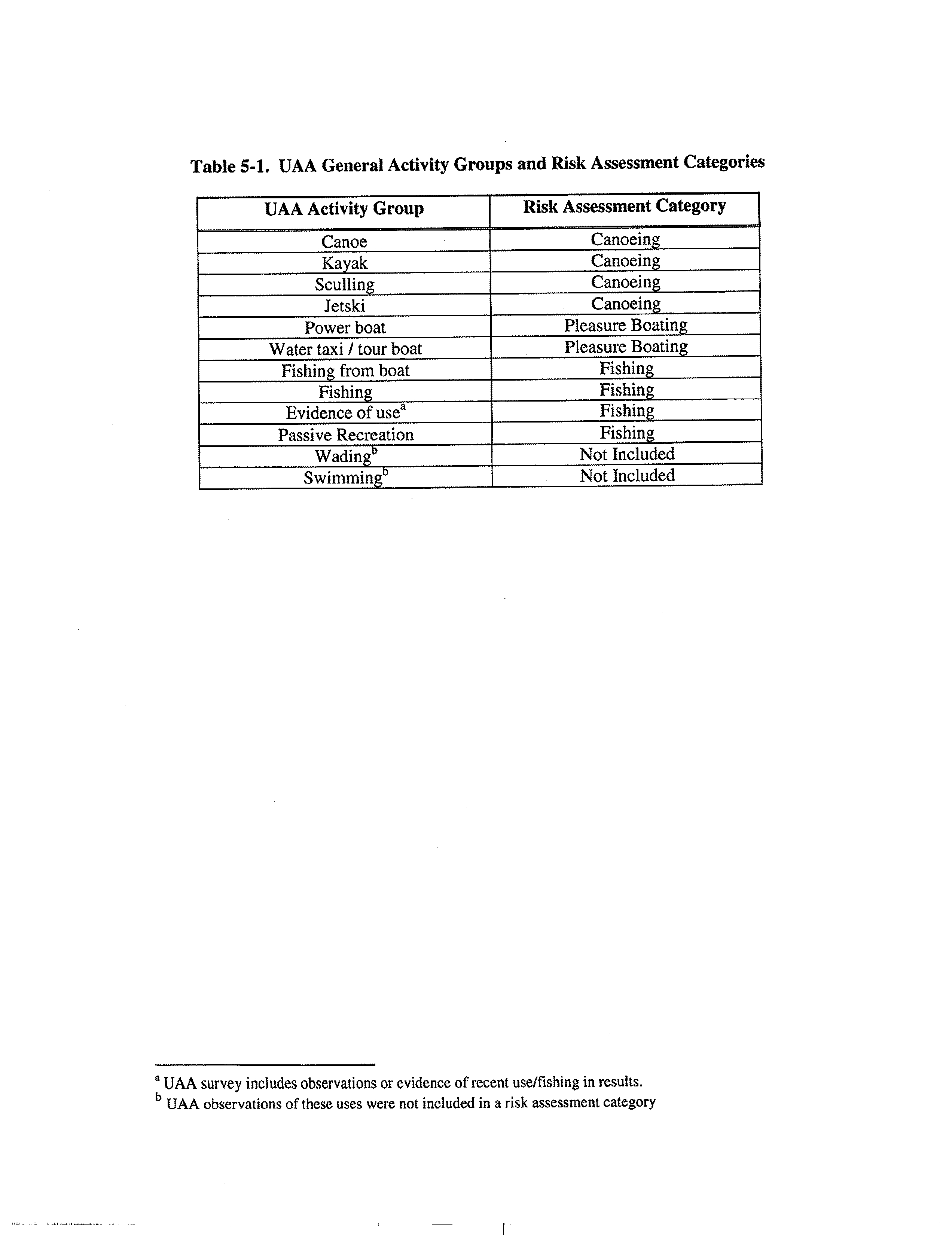
exposure conditions and risks. Recreational survey studies were used to provide insight on the
types and frequency of recreational exposure expected in the waterway. For quantitative risk
analysis,
the UAA study
was the primary source for exposure use data
for the CAWS. As a part
of the UAA, the CAWS
was divided into three major waterway segments each associated with a
single water reclamation plant
-
Stickney
,
North Side and Calumet
.
Recreational use was
divided into high (canoeing
),
medium
(
fishing
)
and low (pleasure boating
)
exposure activities.
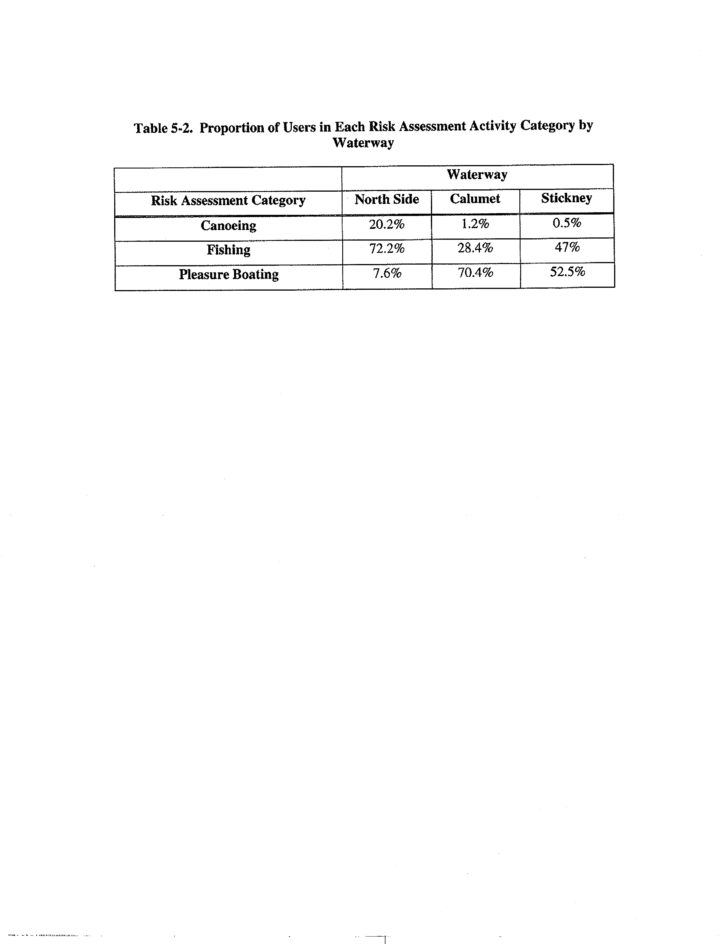
UAA survey
data were used to estimate the proportion of recreational users participating in each
receptor scenario along each waterway segment.
Exposure parameters
,
such as the length of time spent on the waterway and the amount of
water that was incidentally ingested per unit of time spent on the waterway, were developed to
reflect the variability of each receptor scenario as inputs to the exposure model
.
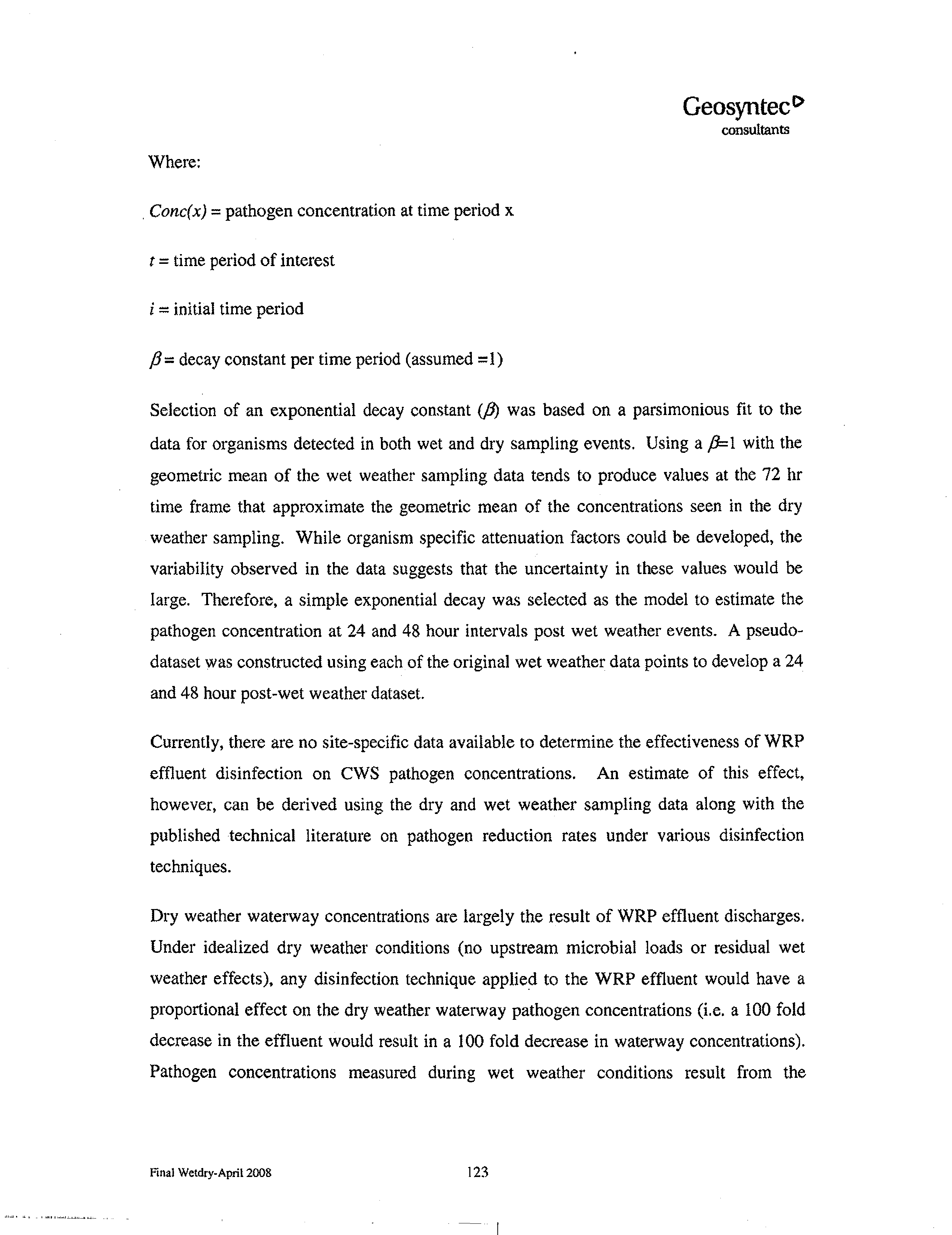
Selection of
input distributions relied on literature derived sources, site-specific use information and
professional judgment.
3
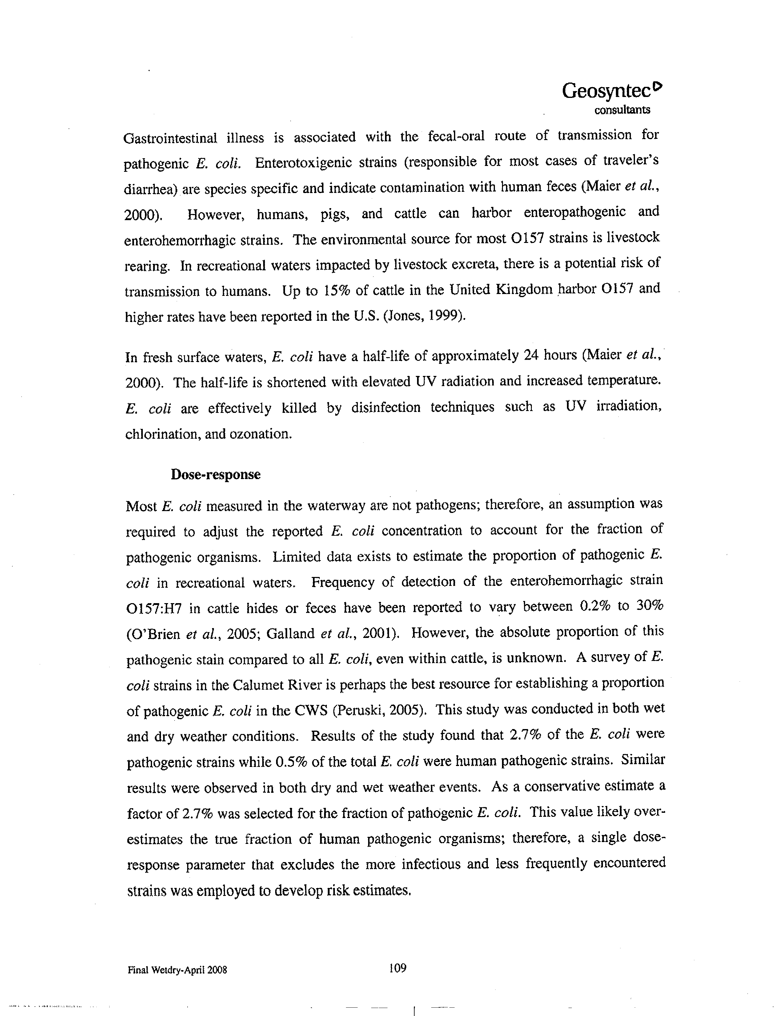
As stated previously, dose-response parameters define the mathematical relationship
between the dose of a pathogenic organism and the probability of infection or illness in exposed
persons.
Dose-response data are typically derived from either controlled human feeding studies
or reconstruction of doses from outbreak incidences. In human feeding trials, volunteers are fed
pathogens in different doses and the percentage of subjects experiencing the effect (either illness
or infection) is calculated.
While feeding trials can provide useful dose-response analysis data,
studies are usually performed in healthy individuals given high levels of a single strain.
Epidemiological outbreak studies provide responses on a larger cross-section of the population,
but dose reconstruction is often problematic. Dose-response relationships for this study were
developed from regulatory documents, industry white papers and peer reviewed literature.
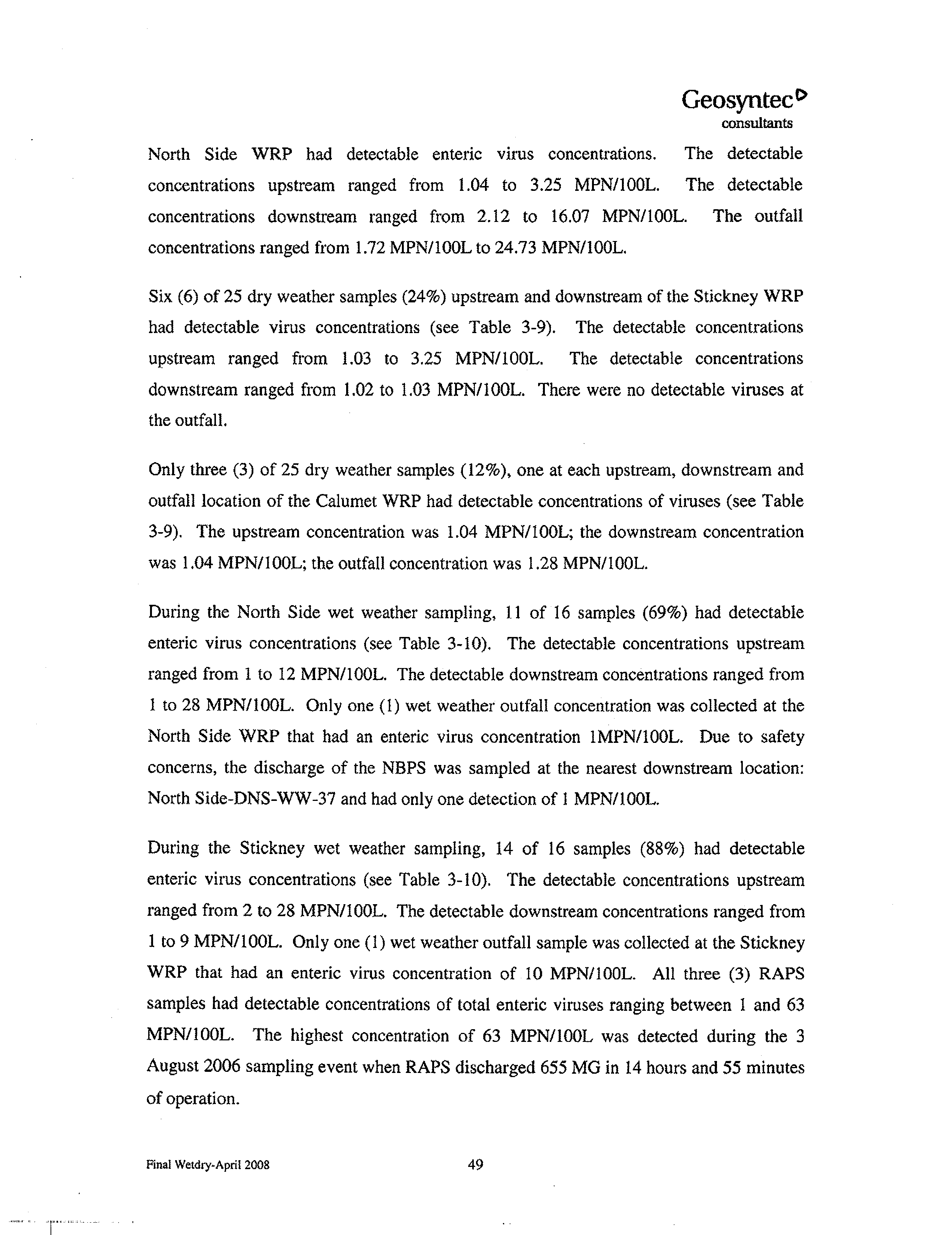
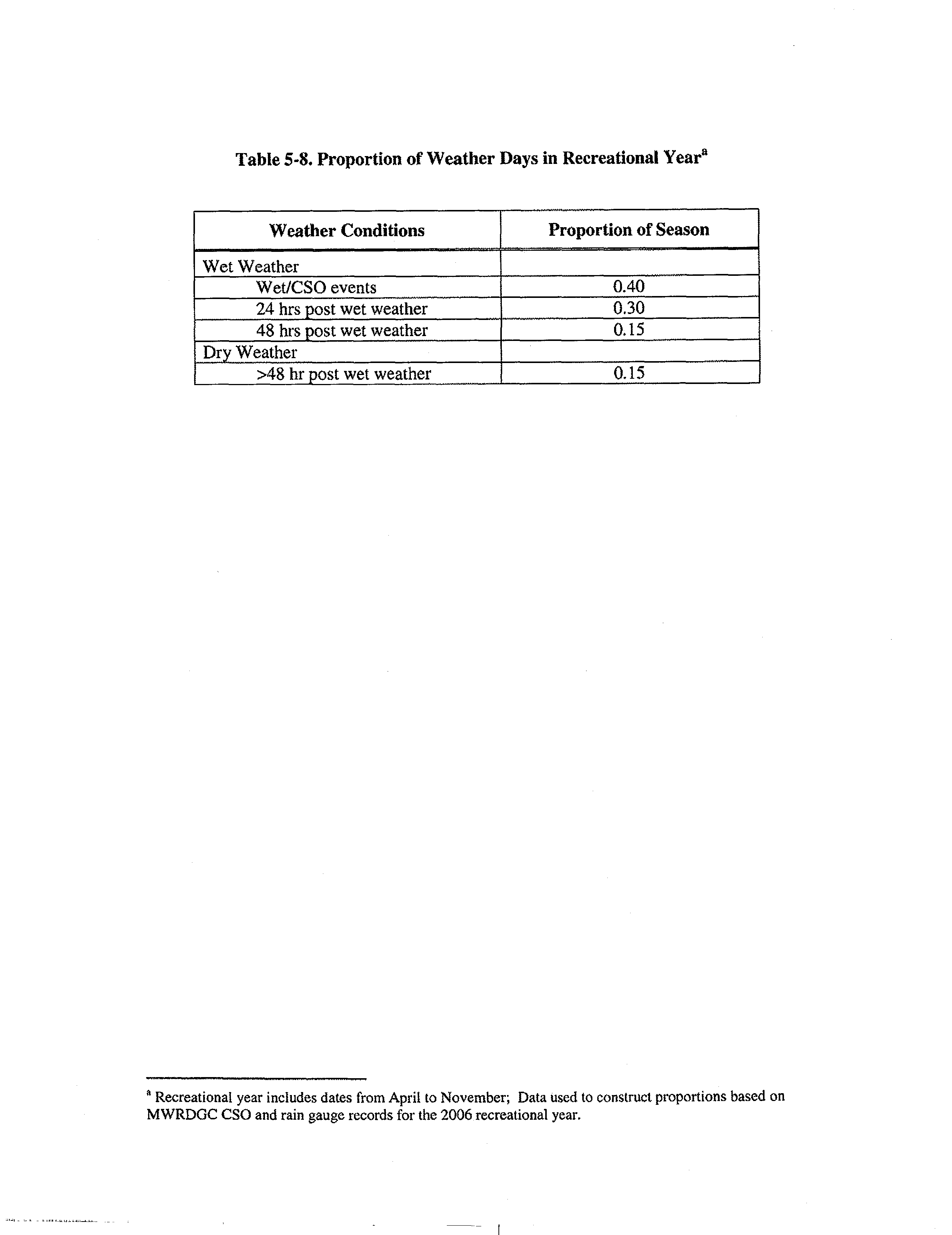
Concentrations of pathogens in the waterway were selected for each simulation from the
entire dataset of dry and wet weather samples collected. The proportion of dry and wet weather
samples utilized were weighted to account for the proportion of dry and wet weather days in a
typical Chicago recreational season.
The methodology used in conducting this study and evaluating the risks of recreational
illness reflect the current state-of-the science in performing quantitative microbial risk
assessment. Similar techniques have been used by the USEPA and other public entities to
support decision making. Components of the methodology and results of this study have been
presented at four national technical conferences and three manuscripts are currently in
preparation for submission to peer reviewed journals.
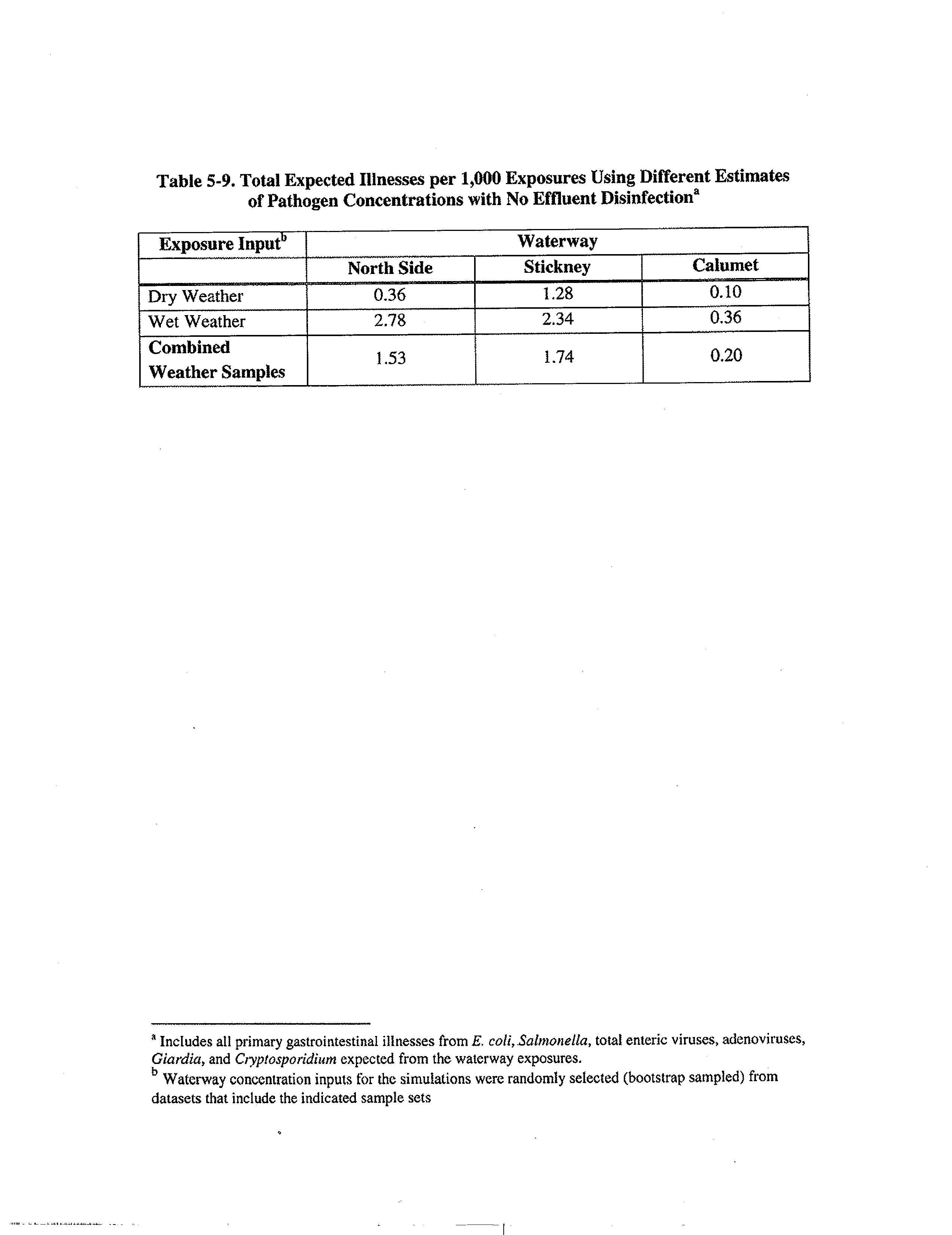
Results of the risk assessment demonstrate that risks to recreational users under various
weather and use scenarios is low and within the U.S. EPA recommended risk limits for primary
contact exposure. The highest rates of illness were associated with recreational use on the
4
Stickney and North Side waterway segments and the lowest illness rate on the Calumet waterway
segment
.
Illness rates were higher under wet weather conditions than under dry weather
conditions.
It is important to note
that the U.
S. EPA has not developed any secondary contact water
quality criteria. However
, the U.S
EPA has proposed a range of primary contact acceptable risk
thresholds and currently has primary contact water quality criteria protective of immersion
activities that is based on an acceptable risk threshold of 8 illnesses per 1000 swimmers
.
This is
the lowest or most stringent of the acceptable risk thresholds used to base water quality criteria
currently adopted by
EPA. The results
of this study demonstrate that the expected illness rates
for receptors were all below
the U.S. EPA's
most conservative acceptable risk threshold illness
rate of 8 illnesses
/
1000 swimmers in primary contact recreational waters.
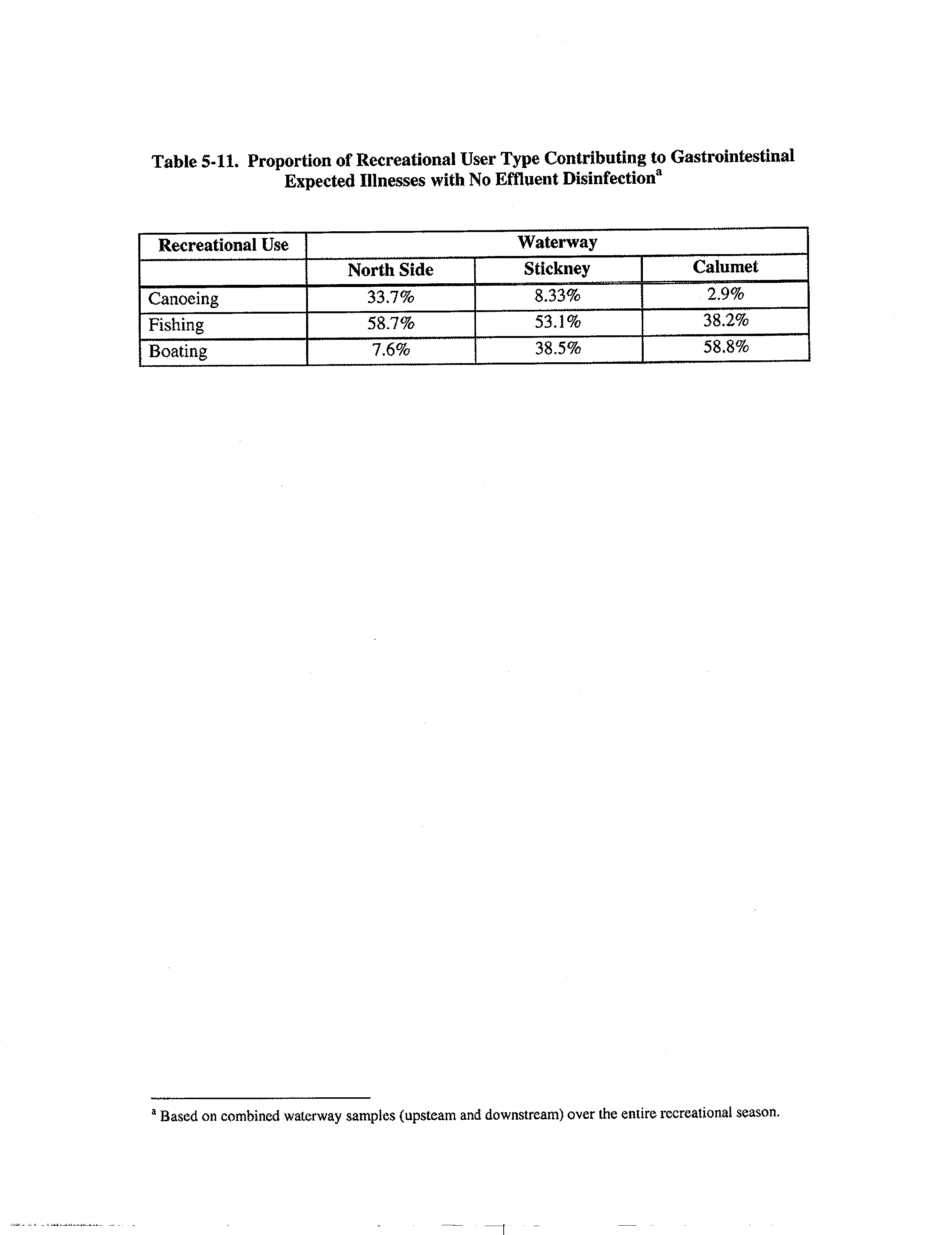
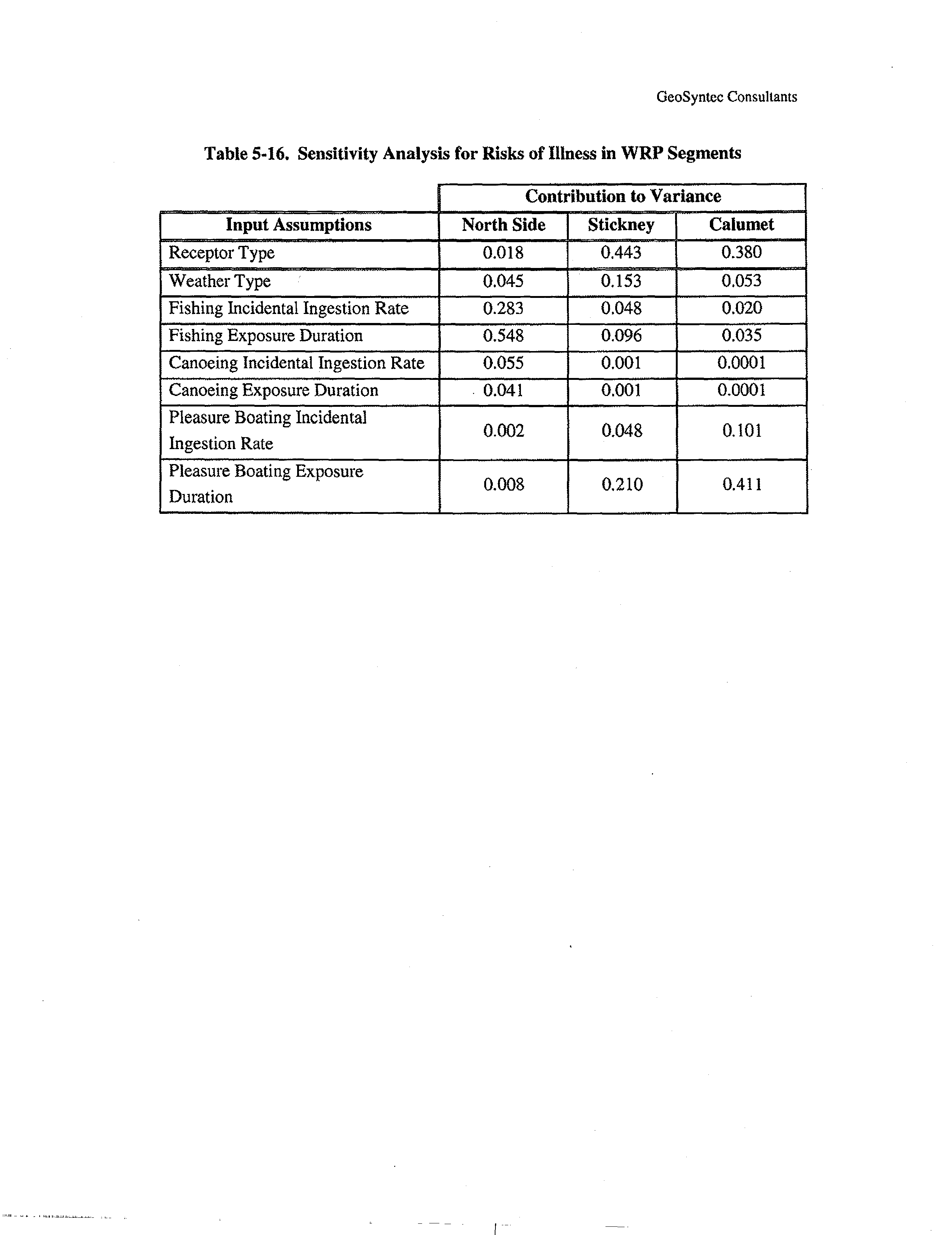
Risks were also calculated individually for each of the three different classes of
recreational use that span the range of exposures reported in
the UAA survey
in proportion to the
frequency of use for each waterway segment
.
The recreational
activity
that results in the greatest
number of affected users depends on both the proportion of users engaged in that activity and the
pathogen load in that waterway segment
.
For example, in the North Side segment
, 33.7% of the
gastrointestinal illnesses are predicted to result from canoeing
,
but canoeing accounts for only
20% of
the users
of the North
Side waterway
.
In the Stickney and Calumet segments, the
predicted illnesses were predominantly from fishing and boating due to the low frequency of
canoeists in these waterway segments
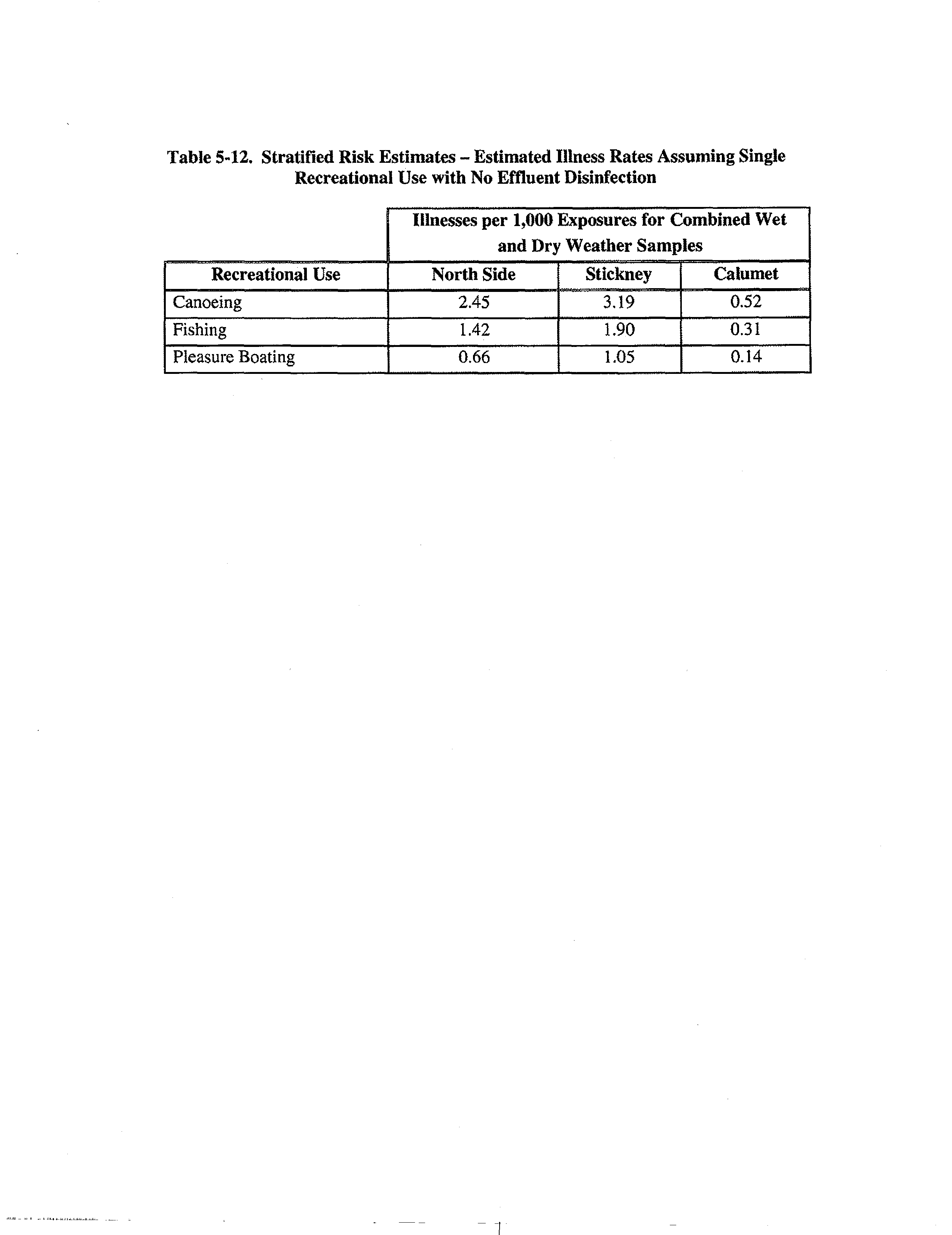
. To further
evaluate the risk stratified by the recreational
use activity, risk per 1000 exposure events were computed separately for canoeing, boating, and
fishing recreational uses.
As expected
,
the highest risks were associated
with
recreational use by
the highest exposure group
(
i.e. canoeing). However
,
for each waterway the risks associated
5
with the highest exposure use are below U.S. EPA's illness rate of 8
illnesses
/ 1000 swimmers in
primary contact recreational waters.
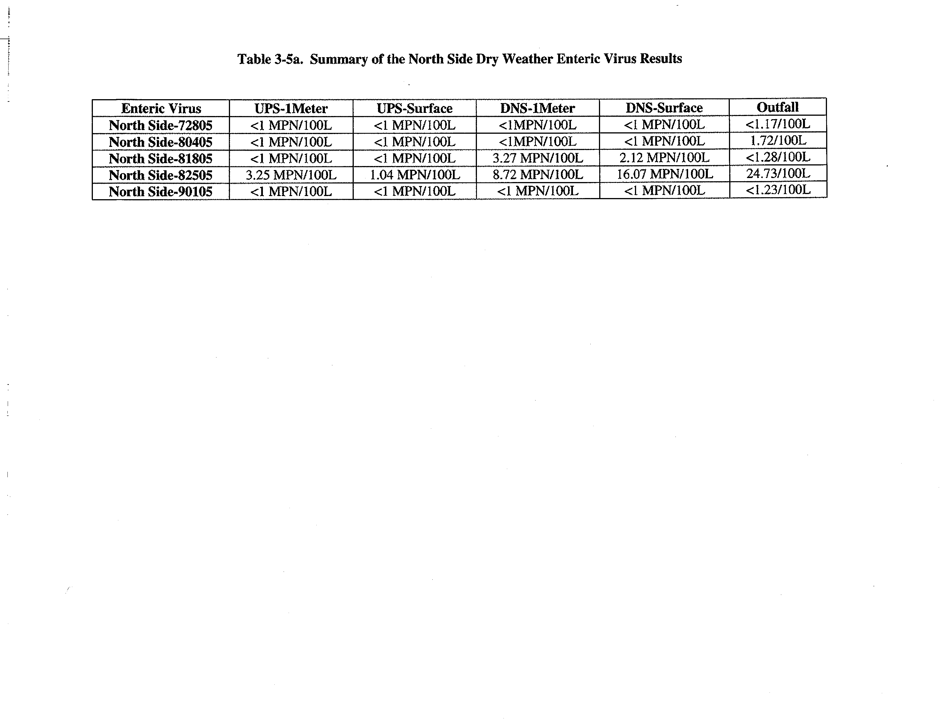
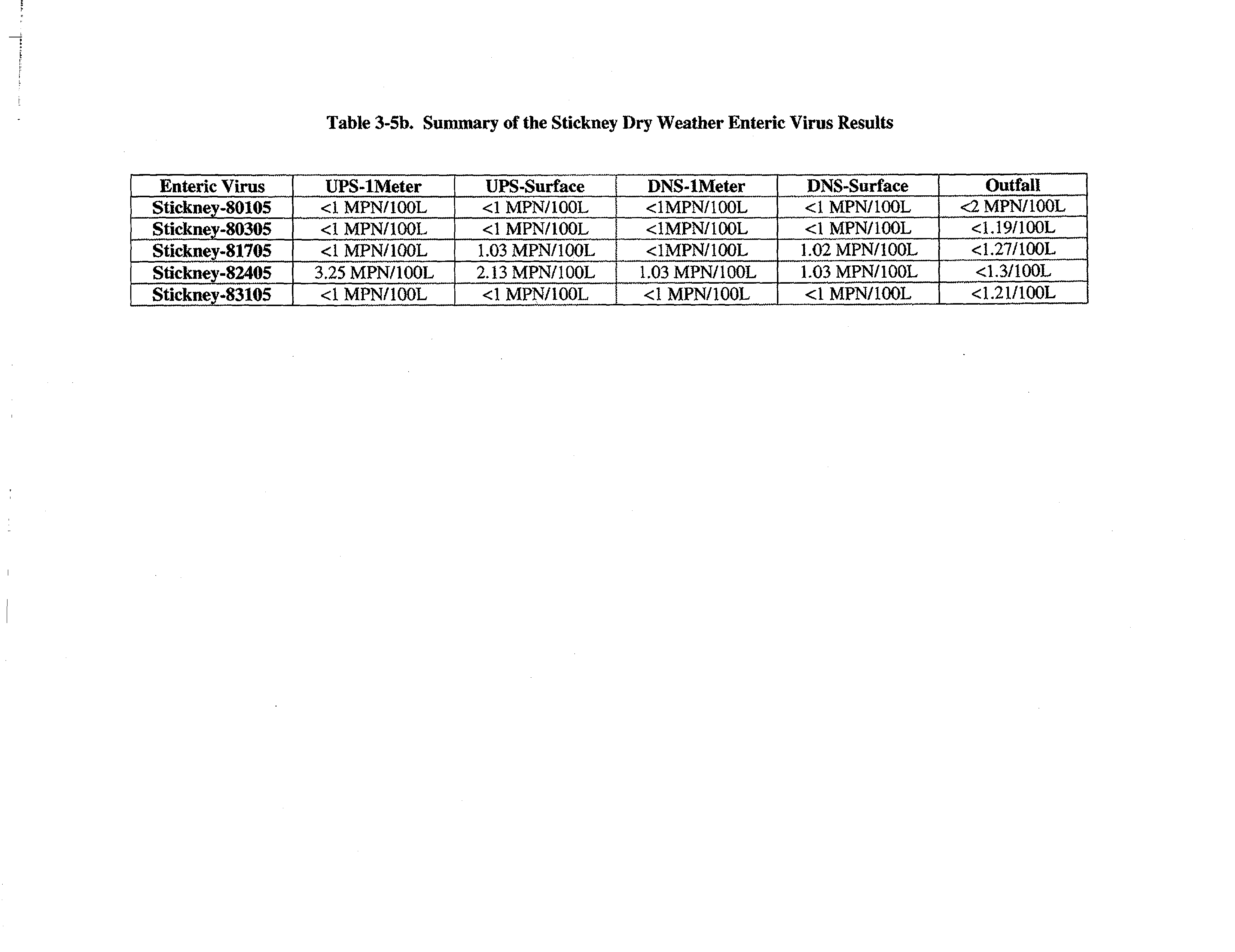
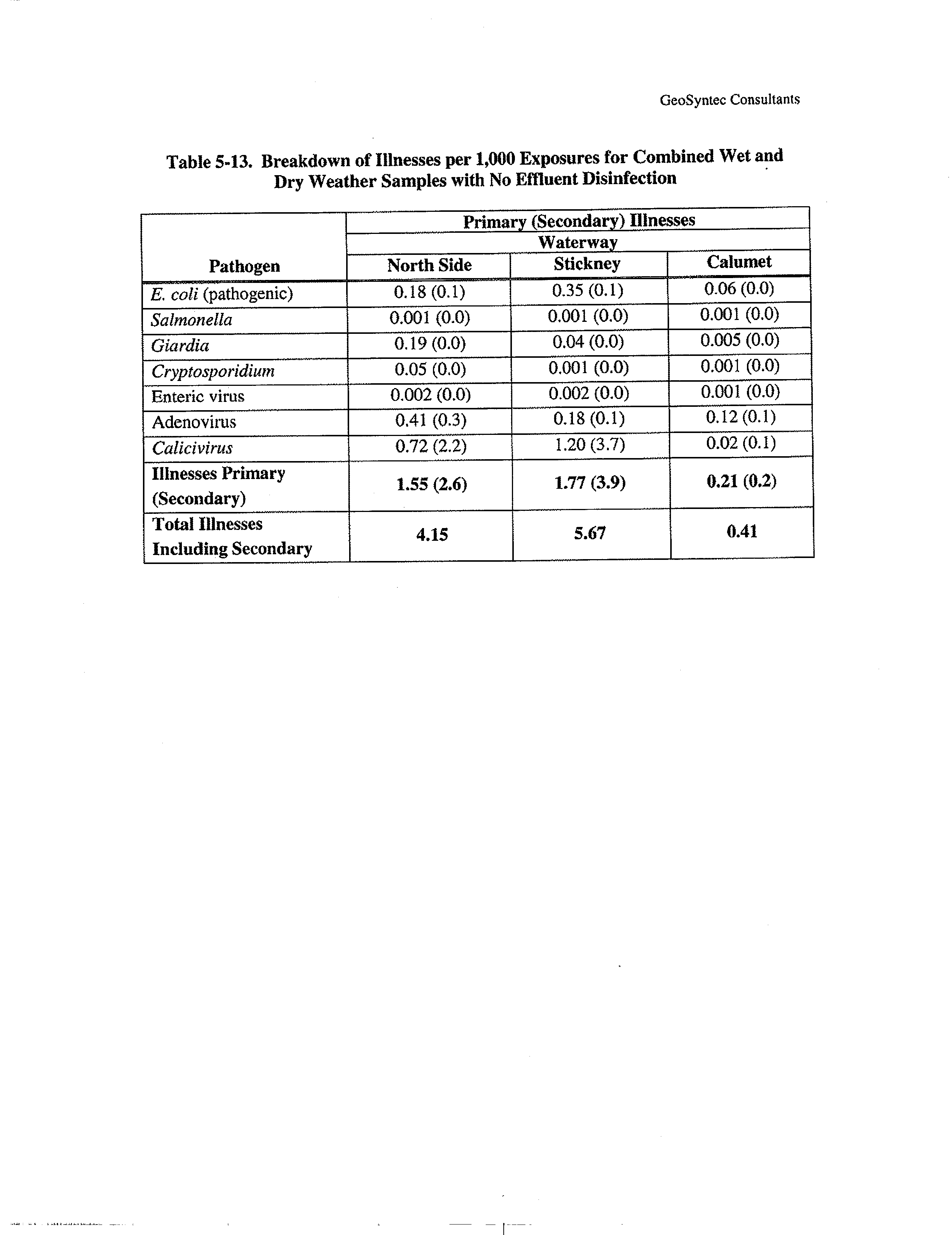
For the North Side and Stickney waterway segments, the majority of predicted
illnesses
were the result of concentrations of viruses, E.
coli
and
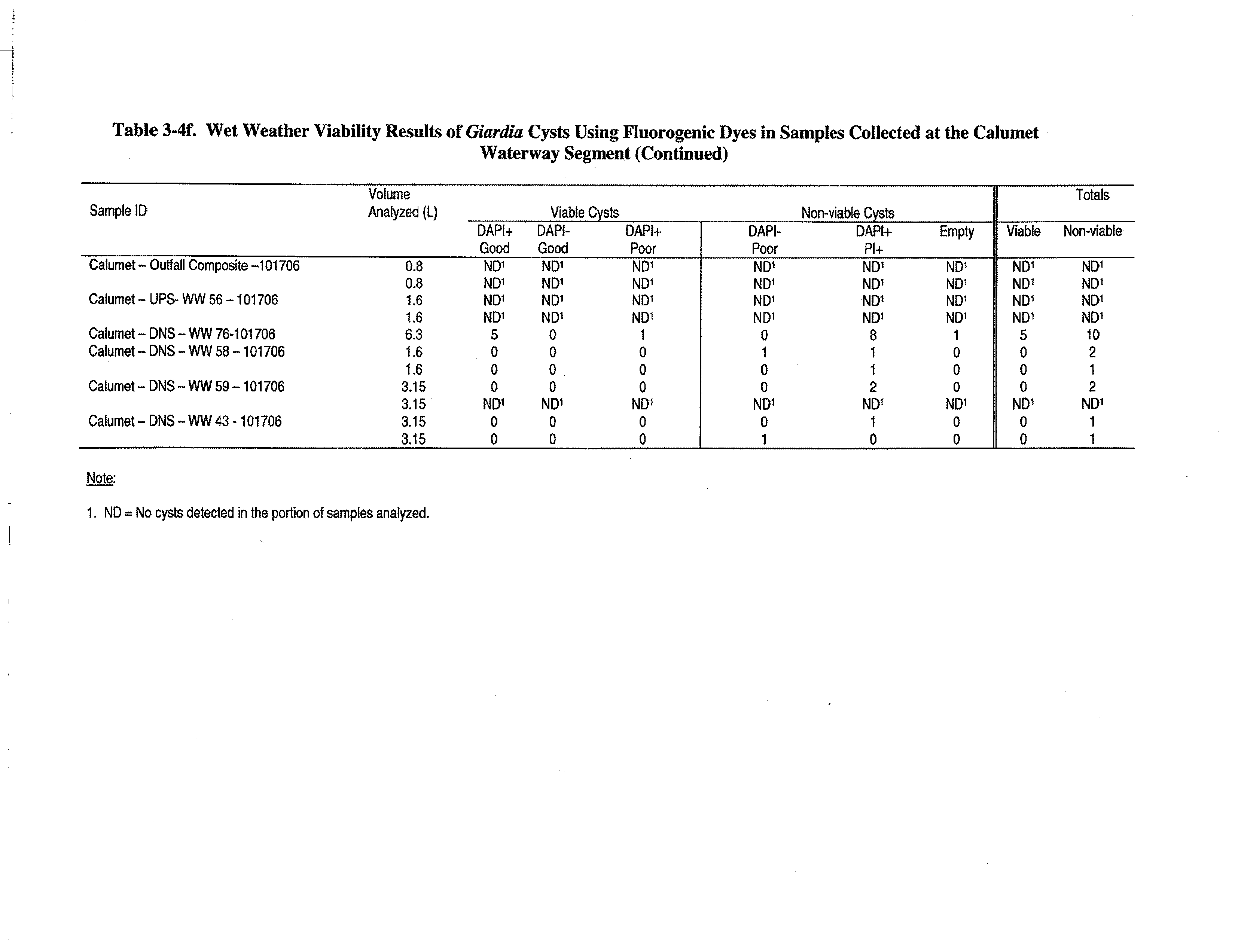
Giardia.
For the Calumet waterway the
risks are generally lower with multiple organisms contributing to overall risk.
Effect of Effluent Disinfection on Pathogen Microbial Risks
The goal of the study was to estimate the effect of disinfection of the effluent from the
water reclamation plants on microbial risk. This was accomplished by evaluating risk under dry
weather conditions when the plant effluent is the major microbial source to the waterway in
addition to wet weather conditions when non-plant inputs are a significant source of microbial
load to the waterway. The plant effluent pathogen loads are similar in both dry and wet weather
conditions such that the dry weather sampling data can be used to estimate the waterway load
that could be affected by disinfection.
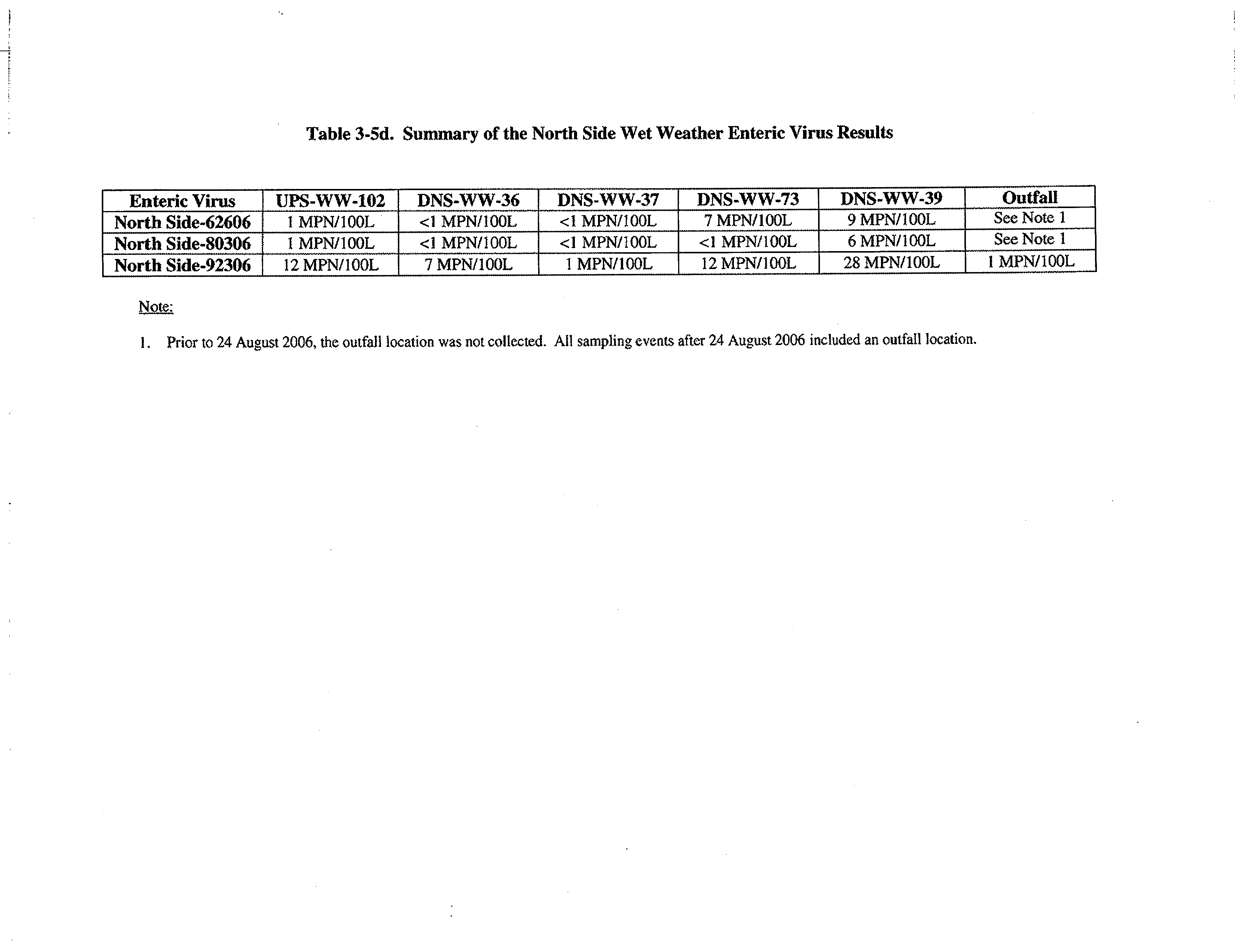
Wet weather sampling data was assumed to encompass
both plant effluent loading (attenuated by disinfection) and non-point discharges to the waterway
(e.g., CSOs, pumping stations, stormwater outfalls).
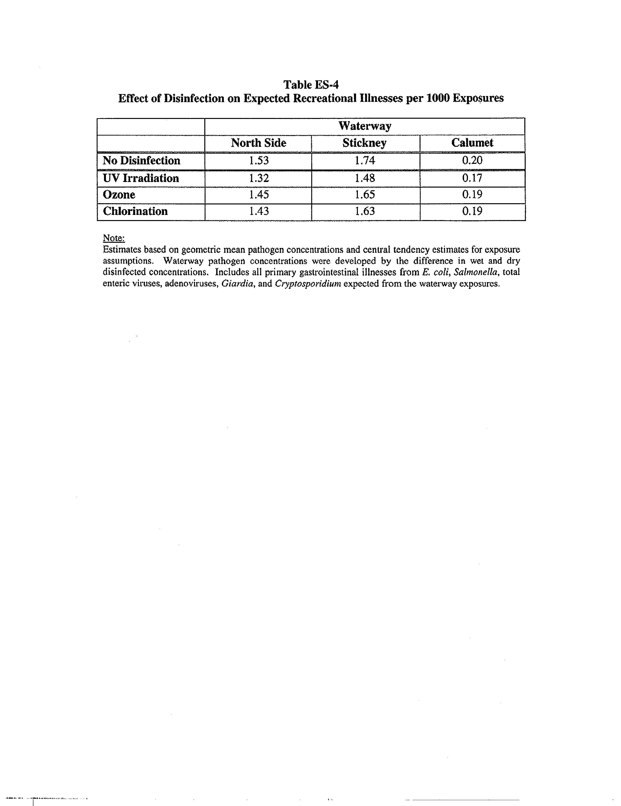
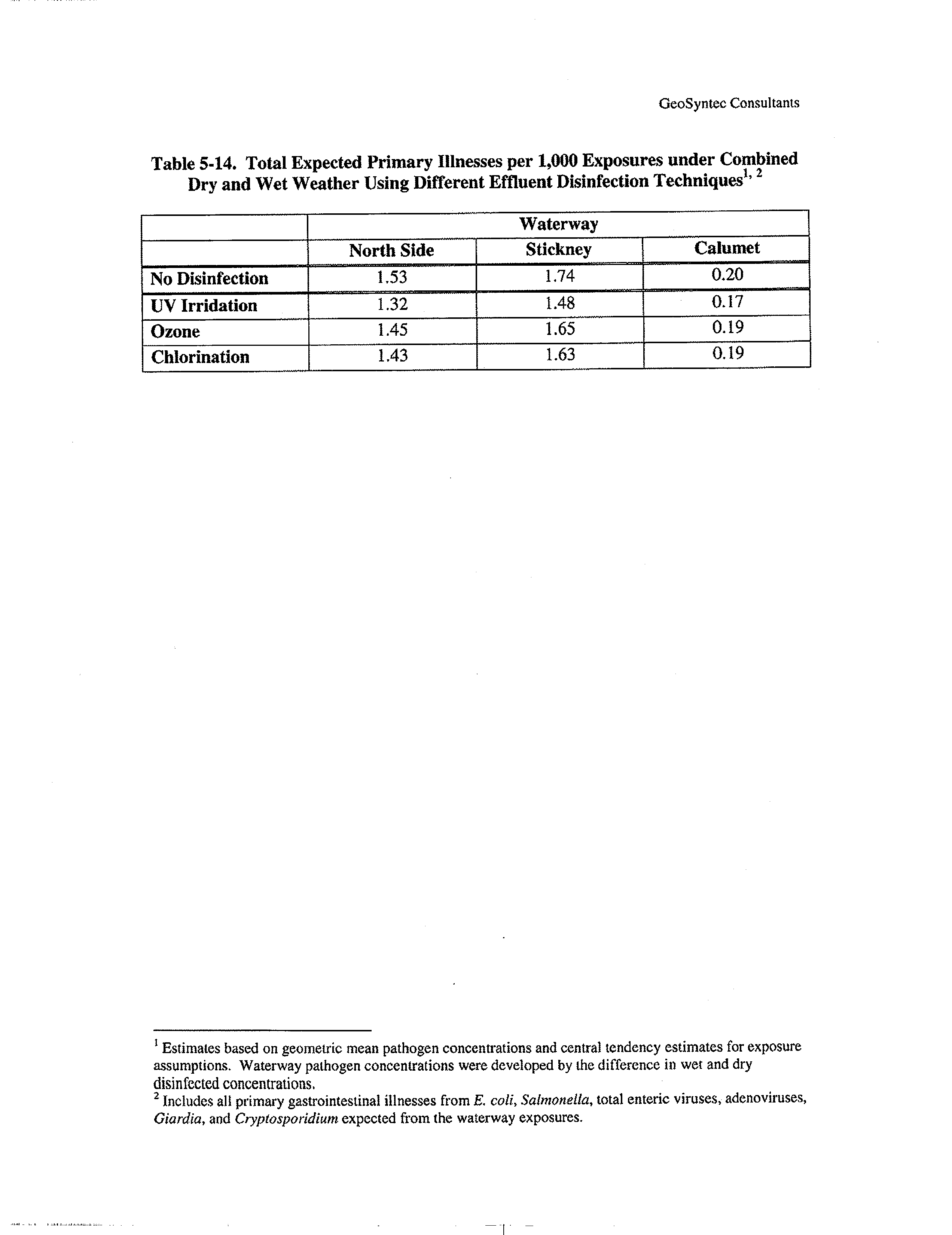
Disinfection of the effluent outfall was predicted to result in a decrease in effluent
pathogen loads from the water reclamation plants but have little effect on overall pathogen
concentrations in the waterway. This is because the sampling data shows that a large proportion
of the pathogen load results from sources other than the plant effluent. Disinfection results in
effluent pathogen risk decreasing from a low level to essentially zero from the water reclamation
plants but has little impact in waterway pathogen concentrations affected by current or past wet
weather conditions. The results are presented in the Table on Exhibit 1. Therefore, these results
suggest that disinfection of effluent will have little impact on the overall
illness
rates from
recreational use of the CAWS.
6
Conclusions
The results presented in my testimony are based on weather and waterway sampling
representative of the entire recreational year. Results demonstrate that, although indicator levels
are relatively high at the water reclamation plant effluents and at locations downstream of the
plants and the North Branch Pumping Station and Racine Avenue Pumping Station, pathogen
levels are generally low. Low pathogen levels correspond to a low probability of developing
gastrointestinal illness, even for the most highly exposed recreational users in areas of the
CAWS in close proximity to non-disinfected effluents from the Stickney, Calumet and North
Side plants. For the designated recreational uses evaluated, the risks of developing illness were
less than U.S. EPA's illness rate of 8 illnesses/ 1000 swimmers in primary contact recreational
waters.
Results further demonstrate that disinfection of WRP effluent will have minimal effects
on overall recreational illness rates.
7
Respectfull
y submitted,
By
J. Keith Tolson, Ph.D.
Testimony Attachments
1.
Exhibit 1. Effect of Disinfection on Predicted
Illnesses
per 1,000 Exposures.
2.
Curriculum vitae
for Dr. J. Keith Tolson.
3.
Dry and Wet Weather Risk Assessment of Human Health
Impacts
of Disinfection vs.
Non-Disinfection of the Chicago Area Waterways System, April 2008.
8
A
tt
ac
hm
e
nt 1
Exhibit 1
.
Effect of Disinfection on Predicted Illnesses per 1
,
000 Exposures
Waterway
North Side
Stickney
Calumet
No Disinfection
1.53
1.74
0.20
UV Irridation
1.32
1.48
0.17
Ozone
1.45
1.65
0.19
Chlorination
1.43
1.63
0.19
Results
•
Overall predicted illness rates are below the EPA criteria (8/1000 exposures).
•
Disinfection has minimal impact on recreational illness rates.
A
ttachm
e
nt 2
Geosyntec'%
consultants
J. Keith Tolson, Ph.D.
EDUCATION
Toxicology
Human and Ecological Risk Assessment
Quantitative Microbial Risk Assessment
Environmental Statistics
University of Florida, College of Medicine, Department of Pharmacology and Therapeutics, Ph.D.
with Specialization in Toxicology
University of Florida, Food Science and Human Nutrition, M.S. (Pesticide Analytical Chemistry
and Forensic Toxicology)
University of Florida, Honors Interdisciplinary Science (Chemistry/Statistics) with Thesis in
Department of Medicine (Division of Pulmonary Medicine), B.S.
PROFESSIONAL HISTORY
Geosyntec Consultants, Tampa, Florida, Director of Toxicology, 2004- present.
University of Florida, Center for Human and Environmental Toxicology, Gainesville, Florida,
Staff Toxicologist, 1997-2004.
University of Florida, Institute of Food and Agricultural Sciences, Gainesville, Florida, Senior
Scientist - Pesticide Research Laboratory, 1991-1997
BIOSKETCH
Dr. Tolson has over 15 years of professional experience in environmental sciences.
His
background experience includes the areas of toxicology, environmental fate and transport, risk
assessment, and statistical modeling.
He is an adjunct professor at the University of Florida
where he serves on the faculty at the Center for Environmental and Human Toxicology. Dr.
Tolson teaches graduate courses in statistics, toxicology and risk assessment.
He has numerous
publications in the field and serves as an editorial reviewer for Risk Analysis, Journal of
Agriculture and Food Chemistry, and Toxicological Sciences.
His professional practice
includes environmental and human health consulting for legal firms, industry and governmental
agencies.
Prior to joining Geosyntec, Dr. Tolson served for eight years as a consultant to the
Florida Department of Environmental Protection, and is co-author of the Department's technical
guidance for Brownfields, Drycleaning, Petroleum, Soil & Groundwater Cleanup Targets, and
Surface
Water rules.
Dr. Tolson was appointed by Florida Governor Charlie Crist to serve as
toxicologist (2007-2011) for the Department of Agriculture and Consumer Services Pesticide
Review Council which is charged with advising the Governor on issues related to the sale, use,
and registration of pesticides in the State.. He has been active at the state and national level
with the development of environmental statistics and toxicological evaluations of legacy
environmental contaminants.
J.
Keith Tolson, Ph.D.
Page 2
REPRESENTATIVE EXPERIENCE
Dr. Tolson has managed toxicology and risk assessment projects, and developed risk-based
strategies for regulatory submission and legal proceedings for municipal and industrial clients.
He has experience in regulatory negotiation and developed quantitative cost-benefit analysis to
support regulatory decision-making.
He has extensive experience with redevelopment issues
associated with former agricultural properties and closed landfills.
He has experience in the
application of RCRA and CERCLA guidance for reports submitted to the USEPA and State
regulatory agencies.
He has managed and/or participated in human health and ecological risk
assessment projects in Alabama, California, Florida, Georgia, Illinois, Kansas, Louisiana, Ohio,
Pennsylvania, Maryland, Massachusetts, Michigan, New Jersey, New York, Tennessee, Texas,
Virginia,
Washington, and West Virginia. Several representative projects are described below:
•
Metropolitan
Water Reclamation District of Greater Chicago, Chicago, IL.
Dr. Tolson
conducted a quantitative microbiological risk assessment for recreational use of the Chicago
area waterways. The analysis was conducted using probabilistic risk assessment techniques
based on site-specific exposure and waterway microbiological sampling.
Monte Carlo
simulations were performed with different microbiological treatment systems to investigate
the human health and ecological effects of various remedial alternatives.
Results of the
analysis will be used by the District to guide them in deciding what, if any, tertiary
treatment will provide a cost-effective reduction in microbiological risks.
The ultimate
decision will involve hundreds of millions of dollars in infrastructure investments and have
regional impacts on water quality.
•
LCP Chemicals of Georgia NPL Site, Brunswick, GA: Project manager for probabilistic
ecological risk assessment at this former chlor-alkali and petrochemical manufacturing
facility.
The site occupies more than 500 acres including terrestrial uplands and an
estuarine marsh adjacent to the Turtle River.
Work included the preparation of a screening
level ecological risk assessment for the upland portion of the site to demonstrate post-
remedial risk reduction, the direction field-sampling activities to support of a large scale
ecological risk assessment for the estuary adjacent to the site.
More than 50 sampling
stations
were evaluated for sediment and surface water chemistry, chronic toxicity of
surface water, chronic toxicity of sediment, benthic invertebrate community structure, and
chemical body burden in a variety of fish, blue crabs, fiddler crabs, marsh grass, and
insects.
A unique element of the ecological risk assessment included the development of
sediment remedial action levels based on site-specific data and probabilistic modeling.
Primary chemicals of concern at this site included mercury, lead, polychlorinated biphenyls
(PCBs), and polycyclic aromatic hydrocarbons (PAHs).
•
Baseline Risk Analysis for Chapter 62-302, Florida Administrative Code. Working for the
Florida Department of Environmental Protection (FDEP) Division of Water Facilities, Dr.
Tolson conducted a probabilistic (Monte Carlo) analysis that incorporated fish consumption
distributions from the Florida Per Capita Fish and Shellfish Consumption Study conducted
by the University of Florida. The analysis used the Florida-specific fish consumption data,
combined with standard toxicity and food-chain biotransfer factors developed by the U.S.
Environmental Protection Agency to estimate cancer and non-cancer health risks to
different segments of the population exposed via their diet to chemicals in surface water at
I Keith Tolson, Ph.D.
Page 3
the State's current standards for non-potable surface water. The risk analysis was used by
FDEP to establish new surface water standards for 25 carcinogenic chemicals and 11 non-
carcinogenic chemicals.
•
Confidential Client Risk Evaluation, Memphis, TN. Dr. Tolson was retained to conduct a
human health risk evaluation of chlorinated pesticides (heptachlor, chlordane,
aldrin/dieldrin, endrin) that were released along a residential corridor over several decades
from a pesticide manufacturing plant during the 1950s and 1960s. Dr. Tolson performed
risk evaluations and negotiated with State and Federal regulators on appropriate remedial
action levels on behalf of client.
Dr. Tolson assisted client and their legal counsel in
strategic planning for regulatory and legal issues as well as communication of complex
health risk information to a concerned public.
Miami-Dade Country Environmental Resource Management, Miami, FL.
Dr. Tolson
conducted a county-wide background study for inorganic compounds to support the County
in making risk-based decisions. Data were analyzed statistically to develop county-specific
background targets.
Results
were compared to regional and national levels and are
currently used to guide site investigation and cleanup activities for sites in South Florida.
Dr. Tolson co-authored the DERM guidance for risk-based corrective action (Chapter 24).
•
Baldwin Station Site - Baldwin, FL.
Dr. Tolson was retained as a testifying expert on
behalf of Southern Wood Piedmont at RCRA permitted facility contaminated with wood
preservatives (arsenic,
pentachlorophenol)
and industrial contaminants (chlorinated
solvents, PAHs, dioxins, pesticides, and other metals).
Southern
Wood is challenging
specific technical elements of a risk-based corrective action regulation promulgated by the
Florida Department of Environmental Protection.
Dr. Tolson was asked to provide expert
toxicology opinions concerning Federal and State risk assessment guidance.
Particular
emphasis was placed on the exposure models and assumptions used to develop risk-based
soil and groundwater remediation levels as well as target cancer and non-cancer risk levels
used to define acceptable human exposure to contaminated media.
•
DuPont de Nemours - Nitro WV. Dr. Tolson was retained by DuPont to conduct a
toxicological profile for bis-(2-chloroethyl) ether (BCEE) in support of lowering the EPA
derived toxicity factor for this compound. EPA initial derived a cancer potency for BCEE
was based on limit studies using older methodology.
A reevaluation using more recent
cancer guidelines suggests that the EPA derived potency factor is several orders of
magnitude too conservative. Successful regulatory approval of the alternative evaluation
allowed the client to safely conclude no remediation of the BCEE plume was required to
protect groundwater resources.
•
Dow Elanco and Gainesville Pest Control Gainesville FL. Dr. Tolson was retained as an
expert toxicologist in a toxic tort case.
Occupants of apartments were exposed to off-label
pesticide application.
Dr. Tolson provided written toxicological profiles and exposure
assessments to support litigation.
•
NASA Kennedy Space Center, FL. Developed KSC-specific cleanup targets for electric
workers exposed to PCBs contaminated soils. Drafted exposure white-paper that accounts
for
worker exposure parameters toxicity information on PCBs, environmental fate and
J.
Keith Tolson, Ph.D.
Page 4
transport of PCBs in and around transformers, and TSCA considerations for residual PCBs
in soils. Successfully defended alternative remediation levels to allow residual PCBs
protective of worker health and the environment.
•
Confidential Client, Ocala, FL.
Dr. Tolson provided expert witness testimony and
consultation in workers compensation cases.
He was retained in cases involving
occupational asthma, chronic solvent exposure, CCA treated wood exposure, worker
accidents involving acute solvent exposures, multiple chemical sensitivity claims and
pyrolyzed plastic exposure.
•
Freshkills Landfill, NY.
The closed Fresh Kills Landfill on Staten Island is a 2,200-acre
site planned for redevelopment as a world-class urban recreation destination, creating the
Fresh
Kills
Lifescape Parkland.
Dr.
Tolson assisted the City in understanding the
environmental and regulatory issues involved in soil contamination used as cover fill.
Dr.
Tolson also was involved in developing remedial targets to define acceptable use areas as a
component of the Site master Plan to support recreational areas, walking paths, cycling
paths, sporting facilities, and nature preserves.
•
Confidential Client, Miami, FL. Dr. Tolson was retained to evaluate the toxicological risks
associated with research chemicals and low level radioactive waste buried at a former
military research facility.
Assisted client and counsel with interpretation of risk issues and
formulation of legal strategy. Participated as toxicological expert in resolution meeting and
subsequent negotiations.
•
HoltraChem NPL Site, Riegelwood, NC: Provided technical support for the Screening Level
Ecological Risk Assessment (SLERA) at a former chlor-alkali facility located on the Cape
Fear River.
Developed a phased field sampling plan with the goal of the reducing the
number of chemicals of potential concern early in the assessment to limit project costs in
later phases of the assessment.
This approach was successful at focusing delineation
sampling to a few chemicals of concern including mercury, PCBs, hexachlorobenzene, and
arsenic.
•
Kennedy Space Center, Cocoa Beach, FL: Provided technical support for the preparation of
human health and ecological risk assessments for multiple SWMUs involving chlorinated
solvents, petroleum products, PCBs, and pesticides/herbicides.
Successfully adapted and
gained regulatory acceptance of a Preliminary Risk Evaluation approach in order to streamline
human health risk assessments and the RCRA Facility Investigation process at the Kennedy
Space Center.
Developed facility-specific ecological risk-based screening levels for
chlorinated pesticides (DDTs, chlordane, heptachlor, aldrin/dieldrin),
metals, PAHs, and
PCBs. FDEP plans to integrate the methods used to develop these screening levels into their
forthcoming ecological risk assessment guidance
•
LA Unified School District, Los Angeles, CA. Assisted District in interpretation and public
dissemination of analytical results associated with construction of new schools. Provided
statistical evaluation on the performance of X-ray fluorescence (XRF) spectroscopy for
field analytical measurements for metals.
Alternative statistical techniques were applied to
assess the ability of XRF to correctly identify a soil sample as above or below acceptable
regulatory criteria.
A dataset was assembled from multiple sites in southern California with
I Keith Tolson, Ph.D.
Page 5
analytical results from both XRF and a fixed-base laboratory. An analysis was conducted to
compare the performance of different statistical techniques to evaluate the suitability of
XRF results compared to the `gold standard' fixed-base laboratory results.
Results of this
analysis showed that alternative method to those suggested in DTSC guidance may provide
a better evaluation of performance.
Results were jointly published with DTSC and may
provide impetus for revision of these rules.
•
Rayonier Wood Treatment Facility, Bunnell, FL.
Dr. Tolson was retained to provide risk
assessment and general consulting to address residual wood treatment contaminants in soil
and groundwater. Site contaminates included arsenic, pentachlorophenol, dioxin, PAHs, and
chromium. Successfully argued that groundwater pentachlorophenol attenuation rates were
higher enough to alleviate the need for costly groundwater remediation.
Used dioxin
fingerprinting analysis to differentiate on- and off-site dioxin sources.
Used a geostatistical
approach to estimate contaminant concentration for the development of site-wide exposure
concentrations.
Developed site-specific alternate soil cleanup target levels (SCTLs) and
demonstrated that proposed remedial actions would achieve Florida's Department of
Environmental Protection's risk targets on a facility-wide basis.
•
Sanford MGP facility, Sanford, FL. Currently assisting client and counsel with regulatory
and PRP group negotiations at a former manufactured gas plant (MGP). Consulting for the
site also includes strategy for dealing with potential human health claims from affected off-
site parties.
Compounds of concern at this site include PAHs, coal tars, wood preservatives,
arsenic, and other metals.
Successfully negotiated with EPA on behalf of client for
exclusion of client as a PRP at the site.
•
Development of Cleanup Target Levels for Chapter 62-777 Florida Administrative Code.
Working for the Florida Department of Environmental Protection Division of Waste
Management, Dr. Tolson and co-workers at the University of Florida served as expert
toxicologists for the State of Florida in developing soil and groundwater cleanup target
levels
for the Department's Petroleum, Drycleaning, and Brownfields remediation
regulations.
The task involved detailed cancer and non-cancer toxicological evaluations of
over 400 individual chemicals.
Cleanup level adjustments were applied for arsenic to
account for recent studies showing that soil bound arsenic is less bioavailable than
previously assumed.
•
LCP Chemicals Inc. NPL Site, Linden, NJ:
Currently
managing the human health and
ecological risk assessments at a former Chlor-alkali facility located on the Arthur Kill,
which is part of the Newark Bay estuarine system. Contaminants at the site include arsenic,
mercury, PCBs, and numerous volatile and semi-volatile compounds.
Work to date has
included preparation of the screening level ecological risk assessment, preparation of a
mercury-soil physiochemical interaction analysis, review of previous assessments prepared
by USEPA Region 2 contractors, preparation and implementation of work plans for the
baseline ecological risk assessment, and providing strategic technical input on site sampling
and analysis for the remedial investigation.
•
Hanlin-Allied-Olin
NPL Site, Moundsville,
WV:
Provided technical support for a
screening-level human health and ecological risk assessments for a former chlor-alkali
J.
Keith Tolson, Ph.D.
Page 6
facility as part of an Engineering Evaluation/Cost Analysis under CERCLA.
Conducted
risk-based GIS mapping to identify areas where potential risks were significant in the
selection of remedial strategies.
The costs associated with several potential remedial
alternatives
were evaluated against the anticipated reduction in site risk following the
"virtual" implementation of each alternative.
This evaluation demonstrated that the most
comprehensive remedial approach did not yield significantly more risk reduction than a less
costly alternative, which was ultimately approved by USEPA.
•
Matthiessen & Hegeler Zinc NPL Site, La Salle, IL: Currently managing the human health
and ecological risk assessment at a former zinc rolling mill and primary zinc smelter located
on the Little Vermillion River. During its operation the facility produced slab zinc, sulfuric
acid, and ammonium sulfate fertilizer.
Manufacturing processes resulted in the emission of
airborne particulate
matter containing PAHs, arsenic, cadmium, lead, zinc and other
inorganic chemicals.
Previously reviewed and commented on the HRS scoring package
prepared by Illinois EPA for this site. Commented specifically on the inappropriate use of
an inhalation cancer slope factor to characterize the potential toxicity of cadmium via the
food chain pathway.
•
Peters Cartridge Factory NPL Site, Kings Mills, OH:
Currently managing the baseline
human health and ecological risk assessment at this former munitions facility located on the
Little
Miami River. For more than 50 years, the facility manufactured semi-smokeless
cartridge ammunition for shotgun, rifle shells. Chemicals of concern primarily consist of
metals such as lead, arsenic mercury, and copper, and volatile organic chemicals associated
with degreasing operations.
Work entails overall site strategy development, risk assessment
work plan preparation and execution, and negations with USEPA and Ohio EPA.
•
Aerojet Facility. Sacramento, CA.
Aerospace research and manufacturing facility with
groundwater and soil contamination resulting from chlorinated solvents use.
Dr. Tolson
provided a probabilistic vapor intrusion risk assessment to define the uncertainty associated
with vapor intrusion analysis to define the extent of remediation needed for protection of
human health. Suitable redevelopment land use designations were assessed for each parcel
based on risk-based assessment and proposed remedial alternatives. Regulatory oversight on
this project was performed by USEPA Region 9 and DTSC.
•
St.
Germain Drum Disposal Sites, Taunton, MA:
Managed human health and ecological
risk assessments for drum burial sites where waste haulers had illegally disposed of drums
containing hazardous waste from multiple facilities in the surrounding area. The sites are
related but geographically separated by short distances.
High concentrations of VOCs in
shallow groundwater plumes triggered concern for the potential vapor intrusion into nearby
residential and commercial buildings.
Conducted vapor intrusion assessments based on a
combination of modeling estimates, soil gas measurements, and indoor air sampling. These
multiple assessment techniques were required because of the complex mix of VOCs in
groundwater and the presence of some of the same chemicals in consumer products used
inside several of the homes and commercial establishments.
•
Fike Chemical NPL Site, Nitro, WV: Provided technical support for the preparation of
human health and ecological risk assessments at a former specialty chemical production
J.
Keith Tolson, Ph.D.
Page 7
facility for a multi-company PRP group.
Assisted in negotiations with regulators from
USEPA Region 3 to establish consensus on risk assessment inputs, particularly the selection
of appropriate exposure assumptions for future industrial redevelopment scenarios.
Developed site-specific soil cleanup target levels and utilized GIS characterization to
demonstrate advantages of targeting remedial actions at isolated areas of elevated dioxin
and arsenic concentrations.
The primary chemicals of concern at the site were
dioxins/furans, arsenic, and chlorinated solvents.
•
Robbins Air Force Base, GA:
Conducted a site-specific risk assessment for soil and
groundwater at a former manufacturing/processing facility.
Developed Type 4 Risk
Reduction Standards (RRS) for all chemicals of concern based on site-specific exposure
conditions.
•
Confederate Park Manufactured Gas Plant, Jacksonville, FL: Provided technical support for
the preliminary human health and ecological risk-based data screening for the contamination
assessment of a former MGP site, currently a city park, located in downtown Jacksonville.
Ecological concerns include impacted sediments in a creek that discharges to the St. Johns
River.
Human health concerns include the consumption of fish from the impacted creek.
Currently assisting the City of Jacksonville in negotiations with FDEP regarding the extent of
additional assessment required.
•
Horse Pasture Site, Robins Air Force Base, GA:
Provided technical support for the
preparation of human health and ecological risk assessments for several SWMUs under
evaluation in the RCRA Facility Investigation process.
Conducted a vapor intrusion
assessment related to potential future commercial and/or residential development of the site.
Negotiated a streamlined ecological risk assessment approach with Georgia EPD based on
limited habitat quality of certain areas of pasture land.
Also successful in negotiating the
exclusion of radionuclides from the formal quantitative risk assessments process. Primary
chemicals of concern at the site included radionuclides, chlorinated solvents, lead, arsenic,
and PAHs.
•
Valley Park, Hagerstown, MD.
Dr. Tolson is currently retained by CSXT to provide
toxicology and risk assessment support for a 120 acre former Koppers Company wood
treatment facility.
Processes on the site included both pentachlorophenol and creosote
treatment of wood. The major treated wood product produced at the site was railroad ties
that were stockpiled over a large area.
The site also contains dioxin residues from
contaminated pentachlorophenol used on-site. Developed site strategy and remedial action
plan for dealing with impacted soils and groundwater.
•
City of St. Augustine, FL. Dr. Tolson is currently assisting the City of St. Augustine with
regulatory compliance issues associated with solid waste management. Dr. Tolson has
represented the City at public meetings to discuss the public health implications associated
with a borrow pit containing fill material and a landfill closed prior to current regulations.
•
C
ry
stal
Springs Park Landfill, Jacksonville, FL. Dr. Tolson was the project toxicologist for
fast-track remedial activities at a City of Jacksonville park located on a former landfill. The
work has included assessment of site soils and groundwater for the presence of dioxins,
metals, PCBs, pesticides, and semi-volatile and volatile organic compounds; and lake fish
J.
Keith Tolson, Ph.D.
Page 8
tissues for the presence of dioxins.
Work also has included design and preparation of plans
and specifications for a presumptive remedy involving placement of a soil cap on over three
acres of a park ball field/picnic area; preparation of human health risk assessments; and
fencing to allow limited park access.
Doeboy Dump Site, Jacksonville, FL.
Dr. Tolson served as project toxicologist for the
assessment and remediation of a 27-acre closed landfill site.
Work completed to date
includes completion of the site assessment and assistance with the Community Involvement
Plan. In addition, Dr. Tolson provided review and interpretation of environmental data to
develop a risk-based strategy to meet human health and ecological criteria for compliance
with FDEP requirements for Site closure.
TEACHING
Dr.
Tolson is an adjunct faculty member at the University of Florida in the Center for
Environmental and Human Toxicology, teaching graduate courses that include:
• Ecological Risk Assessment (VME 6750).
A graduate level course in ecological risk
assessment principle and practice. Guest Lecturer (2005-2008)
•
General Toxicology (VME 6602).
A graduate-level course covering the general
principles of toxicology and mechanisms by which toxic effects are produced in target
organs and tissues. Guest Lecturer. (2000-2007).
•
Advanced Toxicology (VME 6603). A graduate-level course providing a survey of the
health effects of each of the major classes of toxicants.
Guest Lecturer - Pesticides.
(1999-2007).
•
Human Health Risk Assessment (VME 6934). A graduate-level course dealing with the
fundamental concepts, techniques, and issues associated with human health risk
assessment. Guest Lecturer. (1999-2007).
AFFILIATIONS
Society of Toxicology (Food Safety - Executive Committee Member 1998-2002)
Society for Environmental Toxicology and Chemistry
Society for Risk Analysis
American Chemical Society (Agrochemical, Chemical Toxicology)
AWARDS
and COMMENDATIONS
Gamma Sigma Delta, University of Florida Agricultural Honor Society
Sigma Xi, University of Florida Chapter Scientific Honor Society
Phi Theta Kappa, Honor Society
2008 Society of Toxicology Risk Assessment Best Poster Award
2003 University of Florida, Outstanding Graduate Research Award
2001 Society of Toxicology, Food Safety Best Poster Award
2000 Burdock and Associates Toxicology Travel Award
1999 Society of Toxicology Travel Award
J.
Keith Tolson, Ph.D.
Page 9
1998 Society of Toxicology, Risk Assessment Section Best Presentation Award
PUBLICATIONS
1.
DeHaven PJ, RA Siebenmann and JK Tolson. (2008). Geospatial and Bayesian Statistical
Analysis to Enhance Risk-Based Environmental Assessment and Decision-Making.
Proceedings Sixth International Conference on Remediation of Chlorinated and Recalcitrant
Compounds, Monterey CA.
2.
Schuck ME, K Goff, SM Roberts and X Tolson (2008). Geospatial Considerations in
Calculating 95% Upper Confidence Limits on the Mean. Toxicological Sciences 106(1-
S):813.
3.
Tolson, JK, ME Schuck, M DeFlaun, R Lanyon, TC Granato, G Rijal, C Gerba, and C
Petropoulou. (2008).
Microbial Risk Assessment for Recreational use of Chicago Area
Waterways. Toxicological Sciences, 106 (1-S): 121.
4.
Tolson JK, RM Voellmy, and SM Roberts. (2007). Induction of heat stress proteins by
adenoviral mediated gene delivery affords protection to HepG2 cells from hepatotoxicants.
(Submitted: Toxicol. Applied Pharm.).
5.
Tolson JK, CJ Saranko, ME Schuck, and SM Roberts. (2007). Comparison of Tools to
Calculate 95% Upper Confidence Limits on the Mean. Toxicological Sciences 96(1-S):1622.
6.
Saranko CJ, T Bingman, ME Schuck, and JK Tolson. (2007). Evaluation of Current EPA
Cancer Potency Estimates Based on the 2005 Cancer Guidelines. Toxicological Sciences, 90
(1-S):1227.
7.
Custance SR, DJ Oudiz, ME Valenzuela, PA Schanen, TL Watson, and JK Tolson. (2007).
Comparison of XRF and Fixed Base Laboratory Methods for Analysis of Metals.
Toxicological Sciences, 90 (1-S):2008.
8.
Schuck ME, EM Tufariello, CJ Saranko, and JK Tolson. (2007). Acceptable Levels of Risk
-A Survey of State Regulations. Toxicological Sciences, 90 (1-S):1229.
9.
Ettinger R, SC Costello, CL Caulk, JK Tolson. (2007). Quantitative Evaluation of Soil Gas
Profile Data for the Assessment of the Vapor Intrusion Pathway.
Proceeding of the AEHS.
March 19-22.
10. Rijal, G, JT Zmuda, R. Gore, T Granato, C Petropoulou, JK Tolson, C Gerba, RM McCuin,
L Kollias, and R Lanyon. (2007). Dry Weather Microbial Risk Assessment of the Chicago
Area Waterways (CAWS). American Society for Microbiology 107th General Meeting.
11.
JK Tolson, J.K., CP Villaroman, EM Tufariello, SR Custance, R Lanyon, TC Granato, J
Zmuta, G Rijal, and C Petropoulou. (2006).
Probabilistic
model for microbial risk
assessment in recreational waters. Toxicological Sciences, 90 (1-S):1631.
12.
Saranko CJ, JK Tolson, R Budinsky, B Landenberger, SM Roberts, KM Portier. (2006)
Statistical
methods for handling censored dioxin/furan congener data.
Toxicological
Sciences, 90 (1-S):1610.
13.
Tolson JK, S Roy, SM Roberts, and KM Portier. (2006) Age-Specific Estimates of Body
Weights and Surface Areas for Risk Assessments. (Risk Analysis, Accepted: RA-00037-
2006-R1).
J.
Keith Tolson, Ph.D.
Page 10
14.
Tolson JK, DJ Dix, RM Voellmy, and SM Roberts. (2006). Increased Hepatotoxicity of
Acetaminophen in Hsp70i Knockout Mice (Toxicol Appl Pharmacol. 210(1-2):157-62).
15.
Saranko, C.J., Tufariello, E.M., and Tolson, J.K. (2005).
The effect of using multiple
contaminant 95% UCLs on cumulative risk estimates.
Toxicological Sciences, 84 (1-
S):2075.
16.
Tolson, J.K., Saranko, C.J., Roberts, S.M., and Portier, K.M. (2005).
A Robust Algorithm
for Calculating Optimal 95% Upper Confidence Limits (95% UCLs) on the Mean for
Environmental Datasets. Toxicological Sciences, 84 (1-S):2074.
17. Tufariello,
E.M., Saranko, C.J., Ettinger, R., Roberts, S.M., and Tolson, J.K. (2005).
Development of Florida-specific risk-based soil and groundwater cleanup targets for
volatilization of chemicals into indoor air. Toxicological Sciences, 84 (1-S):2073.
18.
Brellenthin, R.P., Tolson, J.K., Kessler, K., and Saranko, C.J. (2005).
Evaluation of the
predictivity of a fish uptake model for mercury using empirical data.
Toxicological
Sciences, 84 (1-S):2076.
19.
Tolson JK, and SM Roberts. (2004). Manipulating Heat Shock Protein Expression in
Laboratory Animals.
Methods. 35(2):149-57.
20.
Tolson JK, Stephen M. Roberts, Bernard Jortner, Melinda Pomeroy and David S. Barber
(2004).
Heat shock proteins and acquired resistance to uranium. Toxicology. 202:172-178.
21.
Tolson, J.K, Saranko, C.J., and Portier, K.M. (2004).
A Systematic Evaluation of
Techniques for Calculating 95% Upper Confidence Limits (95% UCLs) on the Mean.
Presented at the Society of Risk Analysis annual meeting, December, 2004.
22.
Munson JW, JK Tolson, BS Jortner, SM Roberts, and DS Barber. (2003). Heat shock
proteins and uranium nephrotoxicity. Toxicol. Sci. 72(S-1): 1687.
23.
Roy S, JK Tolson, KM Portier, and SM Roberts. (2003). Beefing up - Revised body
weights and skin surface area estimates. Toxicol. Sci. 72(S-1): 1885.
24.
Saranko CJ, CE Mills, JK Tolson, SM Roberts, and KM Portier. (2003). The effect of
censored data on the performance of techniques for calculating 95% upper confidence limits
(95% UCL) on the mean. Toxicol. Sci. 72(S-1): 1915.
25.
Mills CE, CJ Saranko, JK Tolson, SM Roberts, and KM Portier. (2003). Comparison of
techniques for calculating 95% upper confidence limits (95% UCLs) on the mean. Toxicol.
Sci. 72(S-1): 1916.
26.
Tolson JK, DJ Dix, RW Voellmy, and SM Roberts. (2003). Increased hepatotoxicity of
acetaminophen in Hsp70i knockout mice. Toxicol. Sci. 72(S-1): 196.
27.
Roy S, Ochoa HG, JK Tolson, WG Harris, and SM Roberts. (2002). Volatilization of
chemicals from groundwater into indoor air. Toxicol. Sci. 66(1-S):17.
28.
Ochoa-Acuna H, JK Tolson, and SM Roberts. (2002). Dermal exposure to contaminants
while swimming: An assessment of the risks and hazards associated with USEPA Ambient
Water Quality Criteria. Toxicol. Sci. 66(1-S): 102.
29.
Tolson JK, RM Voellmy, and SM Roberts. (2001). Cytoprotection afforded by specific
upregulation of Hsp27 or Hsp70i in HepG2 cells. Toxicol. Sci. 60:345.
J.
Keith Tolson, Ph.D.
Page 11
30.
Tolson JK, RM Voellmy, and SM Roberts. (2000). Overexpression of heat shock proteins
in HepG2 cells using adenoviral gene delivery. The Toxicologist vol. 49:A 201.
31.
Ramaiah SK, JW Munson, JK Tolson, and SM Roberts. (2000). Protein adduct formation
by norcocaine nitroxide, an N-oxidative metabolite of cocaine. The Toxicologist vol. 49:A
204.
32. Halmes
NC, JK Tolson, CJ Portier
,
and SM Roberts. (2000
).
Re-evaluating cancer risk
estimates for short-term exposure scenarios
.
Toxicol
.
Sci. 58:32-42.
33. Tolson
JK, KE
Jordan
,
HG Ochoa, and SM Roberts. (2000
).
Development of Soil Cleanup
Target Levels for Chapter 62
-777, F.A.C.
Division of
Waste
Management, Florida
Department of Environmental Protection
. CEHT
/TR-00-03.
34. Tolson JK, KE Jordan
,
HG Ochoa, and SM Roberts
. (
2000
).
Development of Site
Rehabilitation
Action Standards for Chapter
24 of
the
Miami-Dade County Code.
Department of Environmental Resources
Management
,
Miami
-
Dade County Florida.
CEHT/
TR-00-02.
35.
Tolson JK
, HA Moye, SD
Walker
,
and TS Schubert.
(
2000
).
Phytotoxic effects of Benlate
formulations and N,N'-dbutylurea on ornamental peppers
(
Capsicum sp.).
Pest
.
Sci.52,
287-291.
36.
Tolson JK and SM Roberts. (1999). Cytoprotection from thioacetamide-induced liver injury
associated with heat shock protein induction. Toxicol. Sci. 48:196.
37.
Halmes NC, JK Tolson, CJ Portier, and SM Roberts. (1999).
Re-evaluating cancer risk
estimates for short-term exposure scenarios. The Toxicologist vol. 48:81.
38.
Halmes NC, CJ Saranko, JK Tolson, SM Roberts and RC James. (1999). Baseline Risk
Analysis for Chapter 62-302, F.A.C. (Florida Surface Water Criteria).
Division of Water
Facilities, Florida Department of Environmental Protection. CEHT/TR-99-3.
39.
Saranko CJ, NC Halmes, JK Tolson, and SM Roberts. (1999). Development of Soil Cleanup
Target Levels for Chapter 62-777, F.A.C. Division of Waste Management, Florida
Department of Environmental Protection. CEHT/TR-99-01.
40.
Tolson JK, HA Moye, and JP Toth. (1999). Effect of temperature and humidity on the
formation of N,N'-dbutylurea in Benlate fungicides. J. Agric. Food Chem. Vo147, p1217-
1222.
41.
Tolson JK, JF Gaffney, R Querns, DG Shilling, and HA Moye. (1998). The influence of
benomyl formulation on the response of cucumber seedlings
(Cucumis sativus)
to
Dibutylurea. Pest. Sci. 52, 287-291.
42.
Tolson JK, RM Voellmy, and SM Roberts. (1998). Transgenic mouse model for hepatic
expression of the 27kDa human heat shock protein (HSP27). Toxicol. Sci. 42:372.
43.
Tolson JK, and SM Roberts. (1996). Improving estimates of risk for workers exposed to
contaminated soils at agricultural sites. Fundamental and Applied Toxicology, The
Toxicologist vol 30:A 749. (Presented at the annual meeting of the Society of Toxicology,
1996).
44.
Tolson JK, T Schubert, S Walker, and HA Moye. (1996). Effect of Benlate formulation
type on phytotoxicity to ornamental peppers. Amer. Chem. Soc. 210A344. (Presented at the
210th meeting of the American Chemical Society, Orlando FL, 1996).
J. Keith Tolson, Ph.D.
Page 12
45.
Tolson JK, and HA Moye. (1996). Effect of heat and humidity on decomposition of
benomyl fungicides.
Amer. Chem. Soc. 210A126. (Presented at the 210th meeting of the
American Chemical Society, Orlando FL, 1996).
46.
Tolson JK, HA Moye, and SM Roberts. (1996). Benlate Analytical Data, Formulation
Compositions, and Analysis Protocols. FDEP Contract # HW244-12, HW244-13, HW244-
14, and HW244-15.
47.
Tolson JK, and HA Moye. (1994). Formation of N,N'-dibutylurea from Benlate fungicides.
Amer. Chem. Soc. 206A243. (Presented at the 206th annual meeting of the American
Chemical Society, Chicago IL, 1994).
48.
Shilling DG, HC Aldrich, HA Moye, JF Gaffney, JK Tolson, R Querns, and MA Mossler.
(1993).
N,N' dibutylurea from n-butyl isocyanate, a degradation product of benomyl: II.
Effects on plants. J. Agric. Food Chem. 42:5, pp 1204-1208.
49.
Moye, HA, DG Shilling, HC Aldrich, JE Gander, JP Toth, WS Brey, and JK Tolson. (1993).
Formation of N,N'-dibutylurea from n-butyl isocyanate, a degradation product of benomyl:
1. Formation in Benlate formulations and on plants. J. Agric. Food Chem. 42:5, pp1208-
1212.
50.
Moye HA, A Anderson, T Ali, and JK Tolson. (1992). Stability of pesticides on Empore
extraction cartridges -suitability to remote sampling devices. 3M Grant #FL192.
51.
Hart CM, JK Tolson, and ER Block. (1992). Quantitative fatty acid analysis in cultured
porcine
pulmonary artery endothelial cells:
The combined effects of fatty acid
supplementation and oxidant exposure. JCP 153:76-87..
52.
Tolson, JK, HA Moye, and R Edelstein. (1991). The binding and release of EDB and DBCP
from Florida soils. DER Contract WM-263, USGS publications Grant 14-08-0001-gl663.
53.
Moye HA, and JK Tolson. (1992). Fluorescence enhancement in ordered media. Amer.
Chem. Soc. 204:A35, 1992. (Presented at the 204th annual meeting of the American
Chemical Society, Washington D.C., 1992).
54.
Bhat BG, JK Tolson, and ER Block. (1991).
Hypoxia increases the susceptibility of
pulmonary artery endothelial cells to hydrogen peroxide injury. JCP Vol 151, p228-238.
55.
Hart CM, JK Tolson, and ER Block. (1991).
Supplemental fatty acids alter lipid
peroxidation and oxidant injury in endothelial cells. JAP:LCP. Vol 260, pL483-490.
56.
Bhat GB, SB Tinsley, JK Tolson, and ER Block. (1991).
Mechanism of hypoxia-induced
enhanced susceptibility of pulmonary artery endothelial cells to hydrogen peroxide. Am.
Rev. Respir. Dis. 141:A733, 1991. (Presented at the annual meeting of the American
Thoracic Society, Anaheim, CA, 1991).
57.
Bhat GB, JK Tolson, and ER Block. (1991). Serotonin transport in reconstituted endothelial
cell plasma
membrane proteoliposomes: Effect of hypoxia.
Am. Rev. Respir. Dis.
143:A278, 1991. (Presented at the annual meeting of the American Thoracic Society,
Anaheim, CA, 1991).
58.
Tolson JK, CM Hart, and ER Block. (1991). Fatty acids alter endothelial cell oxidant
susceptibility but not total number of double bonds. Am. Rev. Respir. Dis. 143:A734, 1991.
(Presented at the annual meeting of the American Thoracic Society, Anaheim, CA, 1991).
I Keith Tolson, Ph.D.
Page 13
59.
Hart CM, X Tolson, and ER Block. (1990). Fatty acid supplementation protects pulmonary
artery endothelial cells from oxidant injury. Am. J. Respir. Cell Mol. Biol. Vol 3, p479-483.
60.
Hart CM, JK Tolson, ER Block. (1990). Fatty acids alter the susceptibility of cultured
endothelial cells to oxidant injury. The FASEB J. 4:A839. (Presented at the 74th Annual
Meeting of the Federation of American Societies for Experimental Biology)
61. Tolson
X, ER Block. (1990).
Hypoxia increases the susceptibility of pulmonary artery
endothelial cells (PAEC) to oxidant stress.
Am. Rev. Respir. Dis. 141:A537. (Presented at
the Annual meeting of the American Thoracic Society, Boston, MA, 1990).
62.
Hart CM, JK Tolson, and ER Block. (1990). Supplemental fatty acids affect oxidant injury
and lipid peroxidation in cultured endothelial cells.
Am. Rev. Respir. Dis. 141:A820.
(Presented at the Annual meeting of the American Thoracic Society, Boston, MA, 1990).
"l
Attac
hm
ent 3
Prepared for
Protecting Our Water Environment
Metropolitan
Water Reclamation
District
of Greater Chicago
DRY AND WET WEATHER
RISK ASSESSMENT OF HUMAN HEALTH
IMPACTS OF DISINFECTION VS. NO DISINFECTION OF
THE CHICAGO AREA WATERWAYS SYSTEM (CWS)
Prepared by
Geosy
n
tec "'
con
s
ultant
s
;VIII;
^
.tC^Y,
^t.ti^ti ^ ^11I1C)1'i^^U[S
55 West Wacker Drive, Suite 1100
Chicago,
Illinois 60601
Project Number CHE8188
April 2008
Geosynte&
consultants
TABLE OF CONTENTS
LIST OF TABLES .....................
.................................................................................IV
LIST OF FIGURES ...................................................................................................... VII
LIST OF ATTACHMENTS ..........................................:................................................IX
LIST OF APPENDICES .................................................................................................. X
LIST OF ACRONYMS ...................................................................................................XI
EXECUTIVE SUMMARY .........................................................................................
XIII
1.
INTRODUCTION .....................................................................................................1
1.1
PROJECT OBJECTIVE AND PROJECT TASKS ........................................................... 5
1.2
REPORT ORGANIZATION ....................................................................................... 6
1.3
REFERENCES ........................................................................................................6
2.
MICROBIAL SAMPLING AND ANALYSIS .......................................................
S
2.1
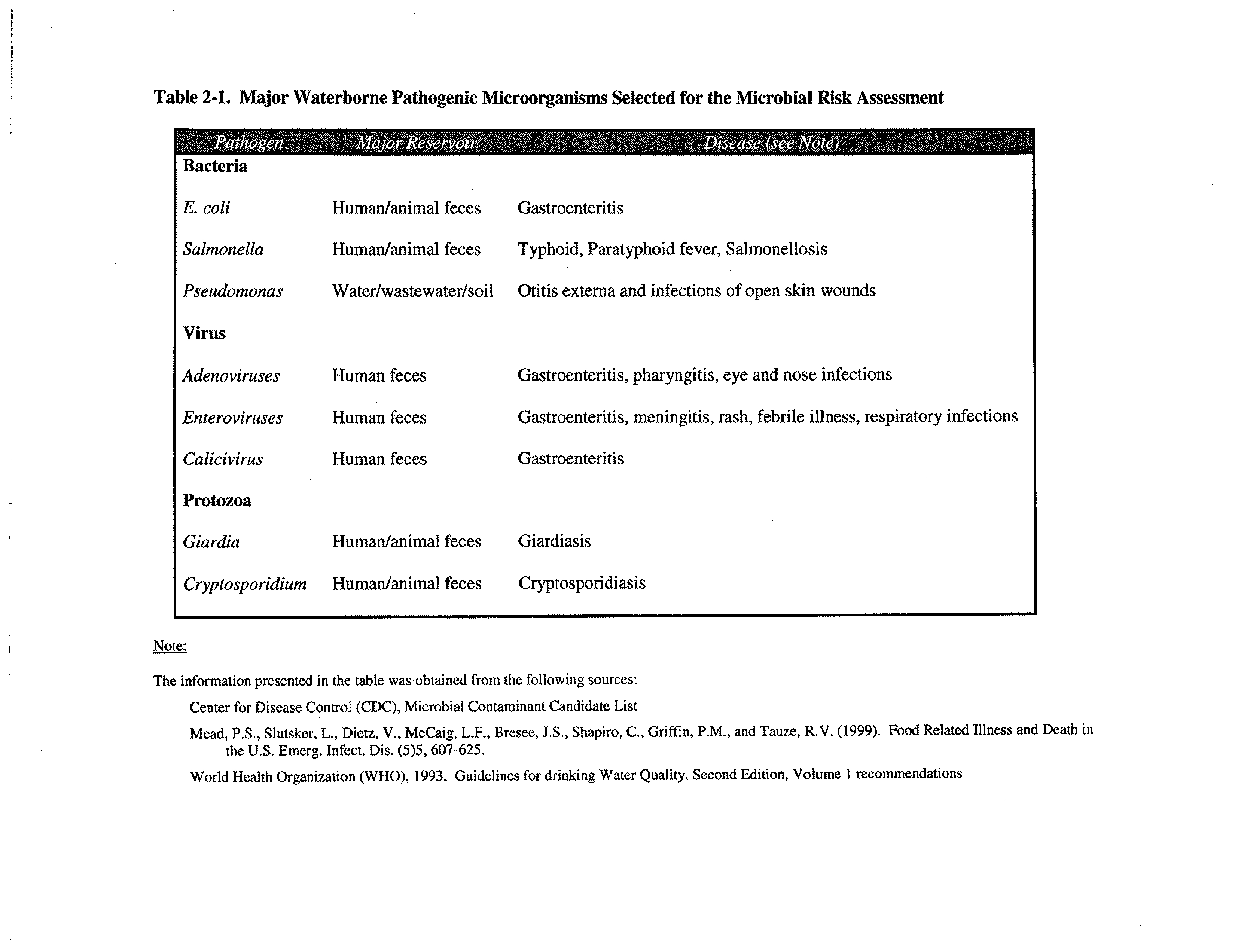
RATIONALE FOR INDICATOR AND PATHOGENIC MICROORGANISM SELECTION .... 8
2.2
SAMPLING OBJECTIVES ........................................................................................ 9
2.2.1
Dry Weather Sampling Objectives ..............................................................9
2.2.2
Wet Weather Sampling Objectives ........................................................... 10
23
FIELD SAMPLING PROCEDURES .......................................................................... 11
2.3.1
Microbial Sampling Locations ..................................................................11
2.3.1.1
Dry Weather Sampling Locations .........................................................12
2.3.1.2
Wet Weather Sampling Locations .........................................................14
2.3.2
Sample Collection Equipment, Materials and Procedures ........................15
2.3.2.1
Virus Sampling ...................................................................................... 19
2.3.2.2
Bacteria Sampling ................................................................................. 20
2.3.2.3
Cryptosporidium
and
Giardia
Sampling ...............................................20
2.3.3
Sample Identification ................................................................................ 22
2.3.4
Sample Custody .........................................................................................22
2.3.5
Sample Packaging, Shipment, and Tracking ............................................23
2.3.5.1
Sample Packaging ................................................................................23
2.3.5.2
Shipping and Tracking .......................................................................... 24
2.3.6
Waste Management ...................................................................................24
2.3.7
Health and Safety ...................................................................................... 24
2.4
QUALITY ASSURANCE/ QUALITY CONTROL PROCEDURES ................................. 25
2.4.1
Microbial Methods of Analyses ................................................................ 25
2.4.2
Data Quality Objectives ............................................................................ 26
2.4.3
QA/QC Procedures ....................................................................................26
2.4.3.1
Laboratory Internal QC ......................................................................... 27
2.4.3.2
Equipment Calibration .......................................................................... 31
2.4.3.3
Equipment Maintenance ........................................................................ 31.
2.4.3.4
Corrective Actions ................................................................................. 31
Final Wetdry
-
April 2008
i
TABLE OF CONTENTS
(Continued)
2.5
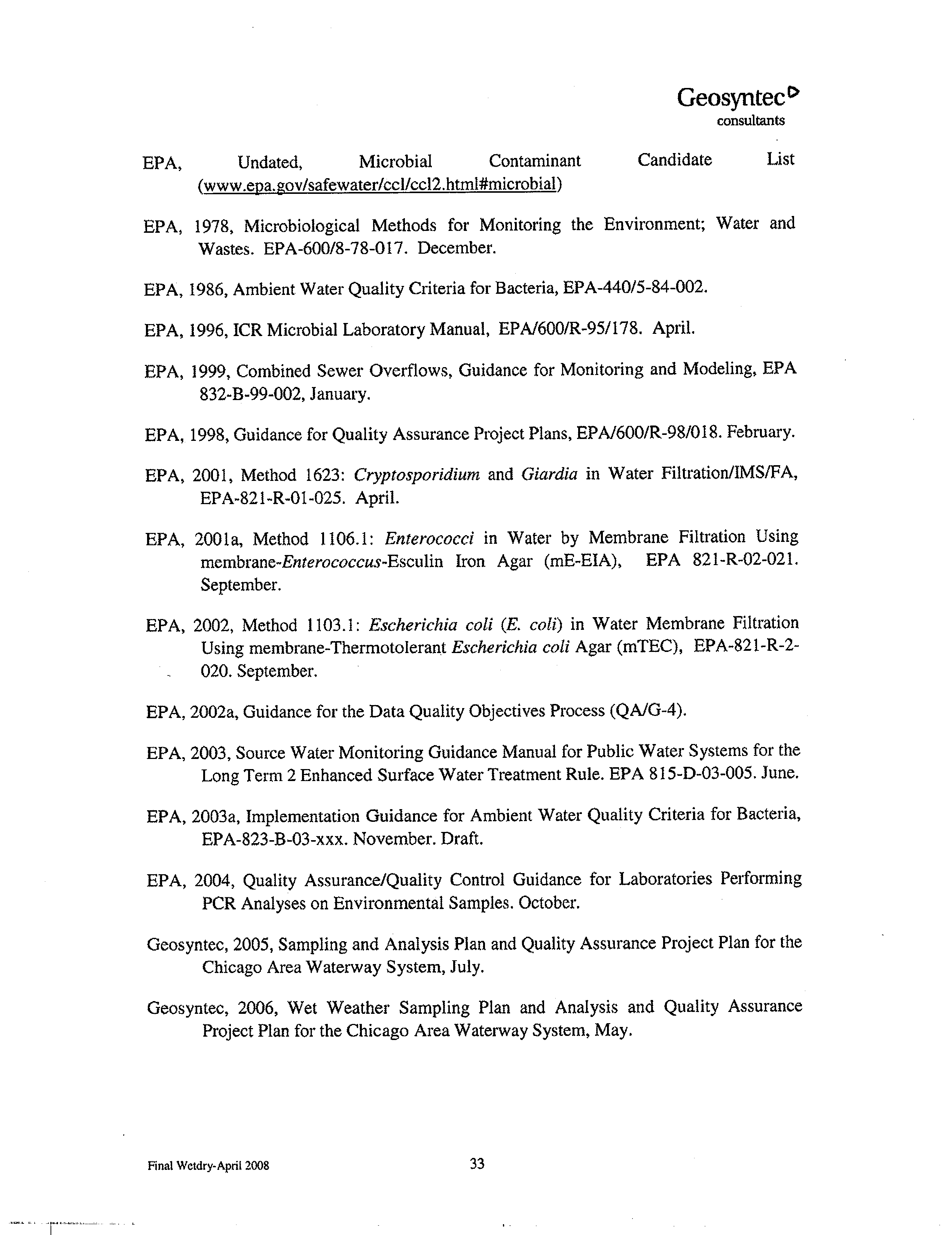
REFERENCES ...................................................................................................... 32
3.
ANALYTICAL RESULTS
.....................................................................................35
3.1
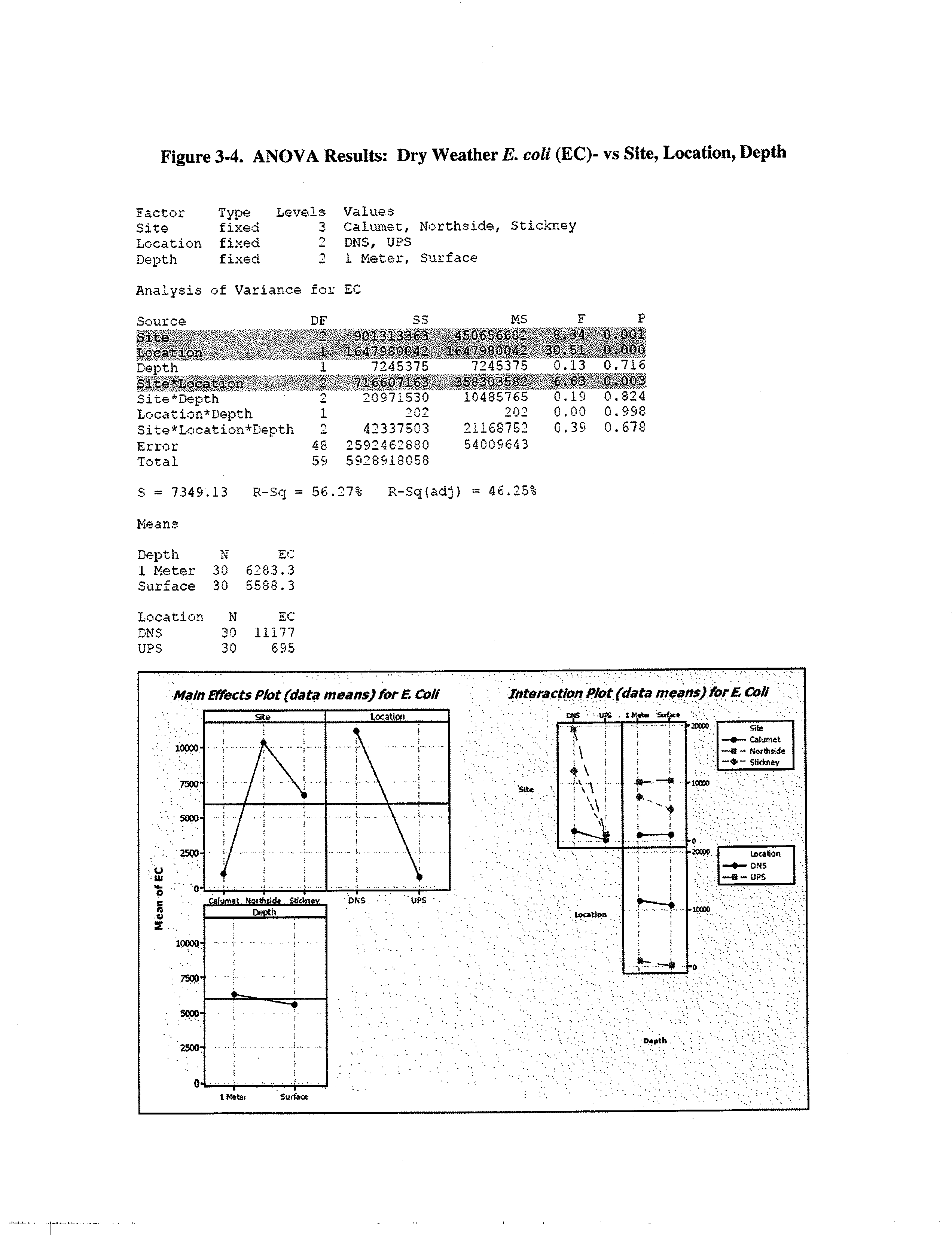
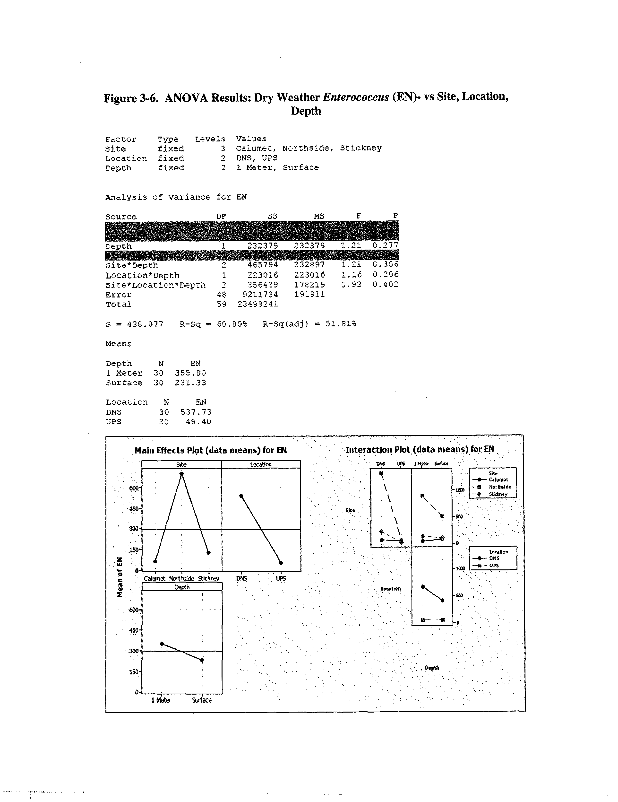
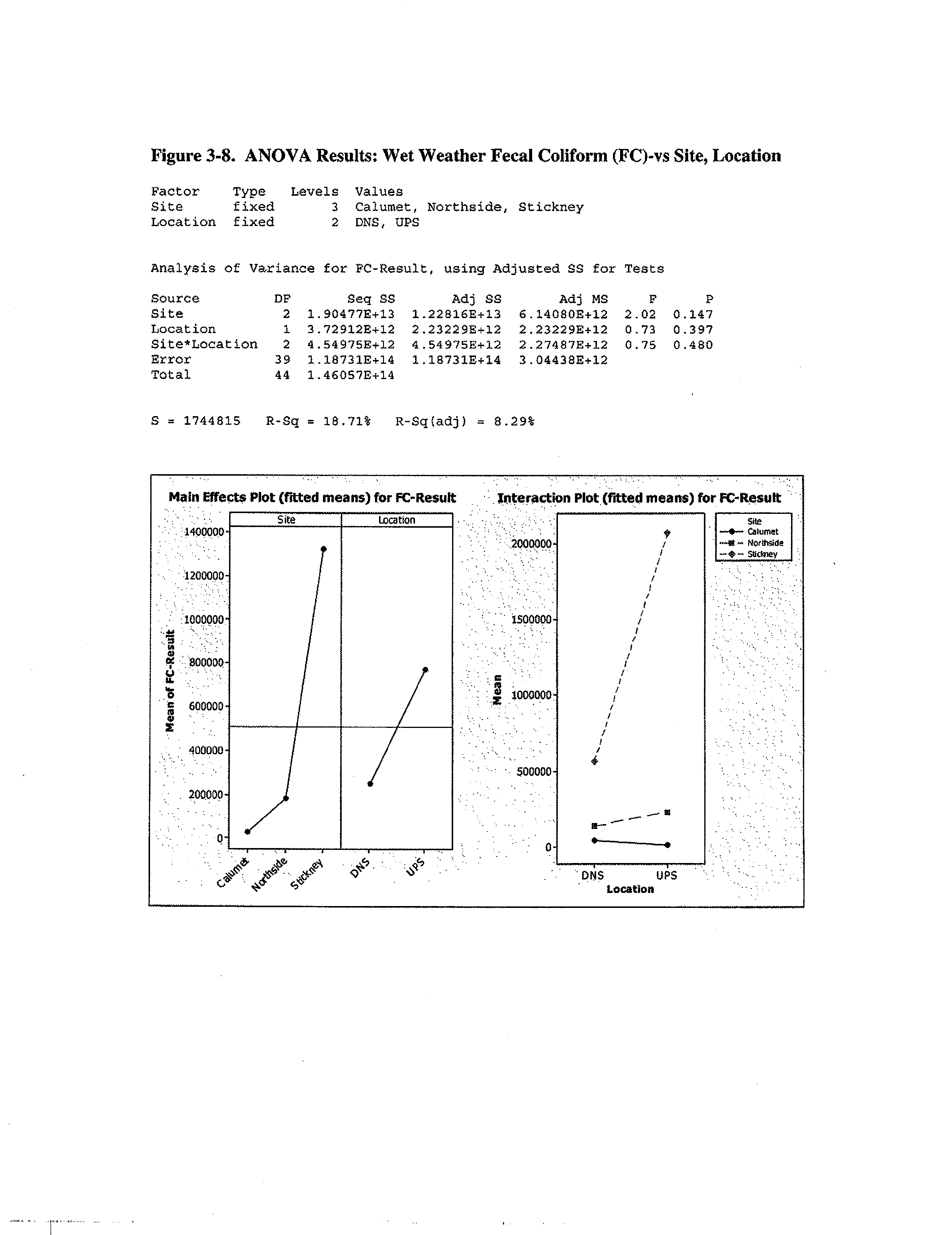
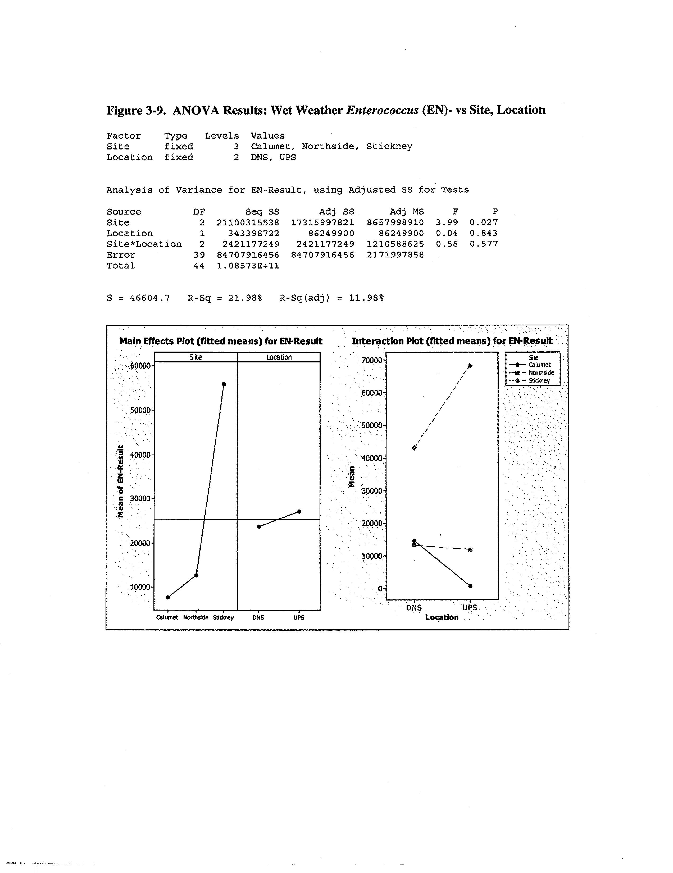
BACTERIA RESULTS ........................................................................................... 35
3.1.1
Analysis of Variance (ANOVA) ............................................................... 36
3.1.2
Geometric
Means
...................................................................................... 39
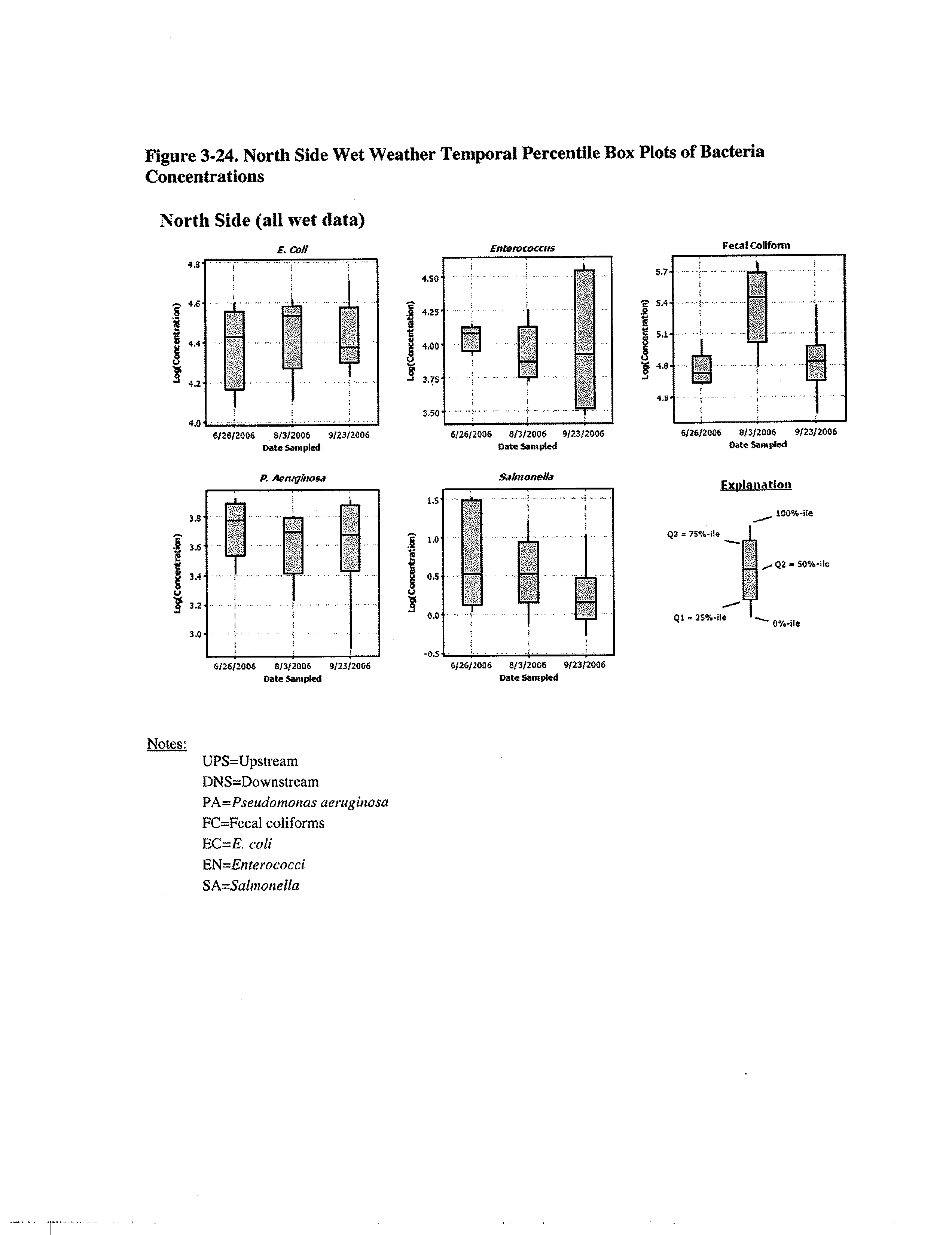
3,13
Percentile Box Plots .................................................................................. 40
3.2
PROTOZOA ANALYTICAL RESULTS ..................................................................... 41
3.2.1
Enumeration Results .................................................................................41
3.2.2
Detection of Infectious
Cryptosporidium
Oocysts Using Cell Culture.... 43
3.2.3
Giardia
Viability Results .......................................................................... 44
3.3
VIRUS ANALYTICAL RESULTS ............................................................................ 47
3.3.1
Enteric Viruses ..........................................................................................48
3.3.2
Adenovirus ................................................................................................ 50
3.3.3
Calicivirus
(Norovirus) ............................................................................. 52
3.4
REFERENCES ...................................................................................................... 55
4.
DISINFECTION
.....................................................................................................
58
4.1
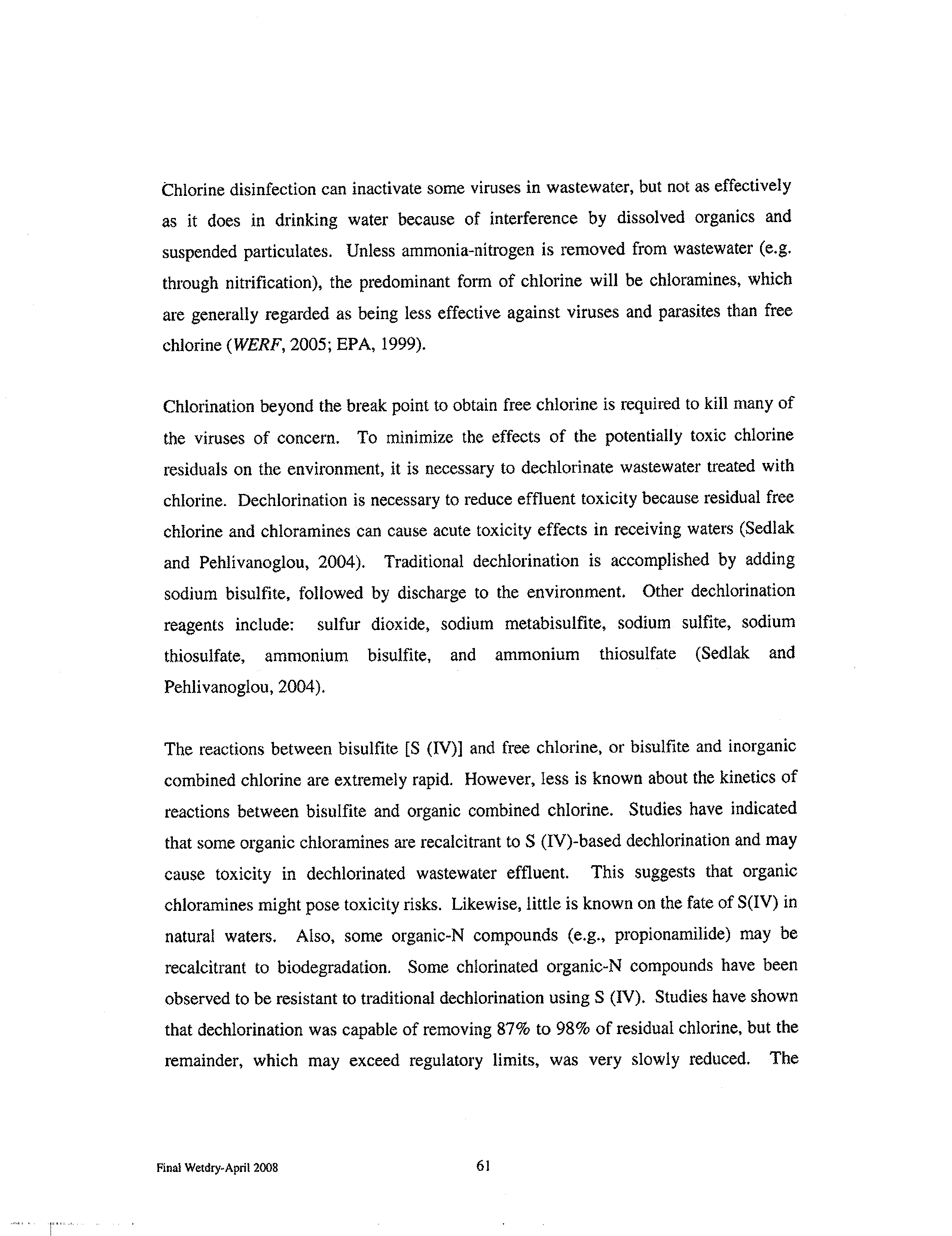
CHLORINATION/D1CHLORINATION .................................................................... 59
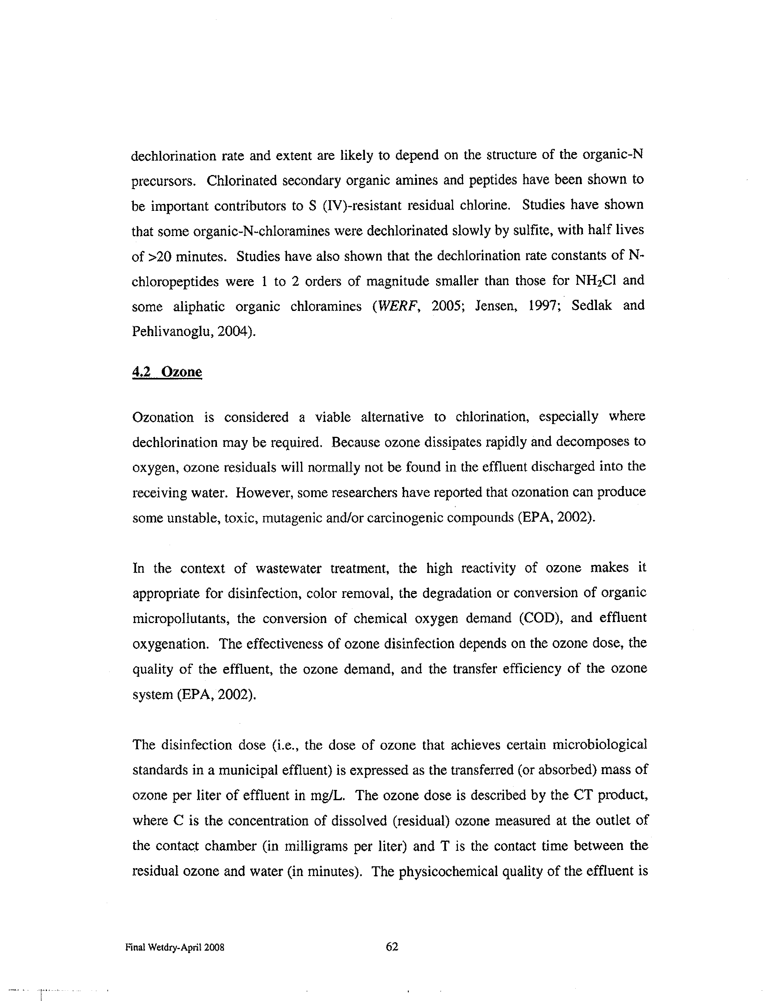
4.2
OZONE ................................................................................................................62
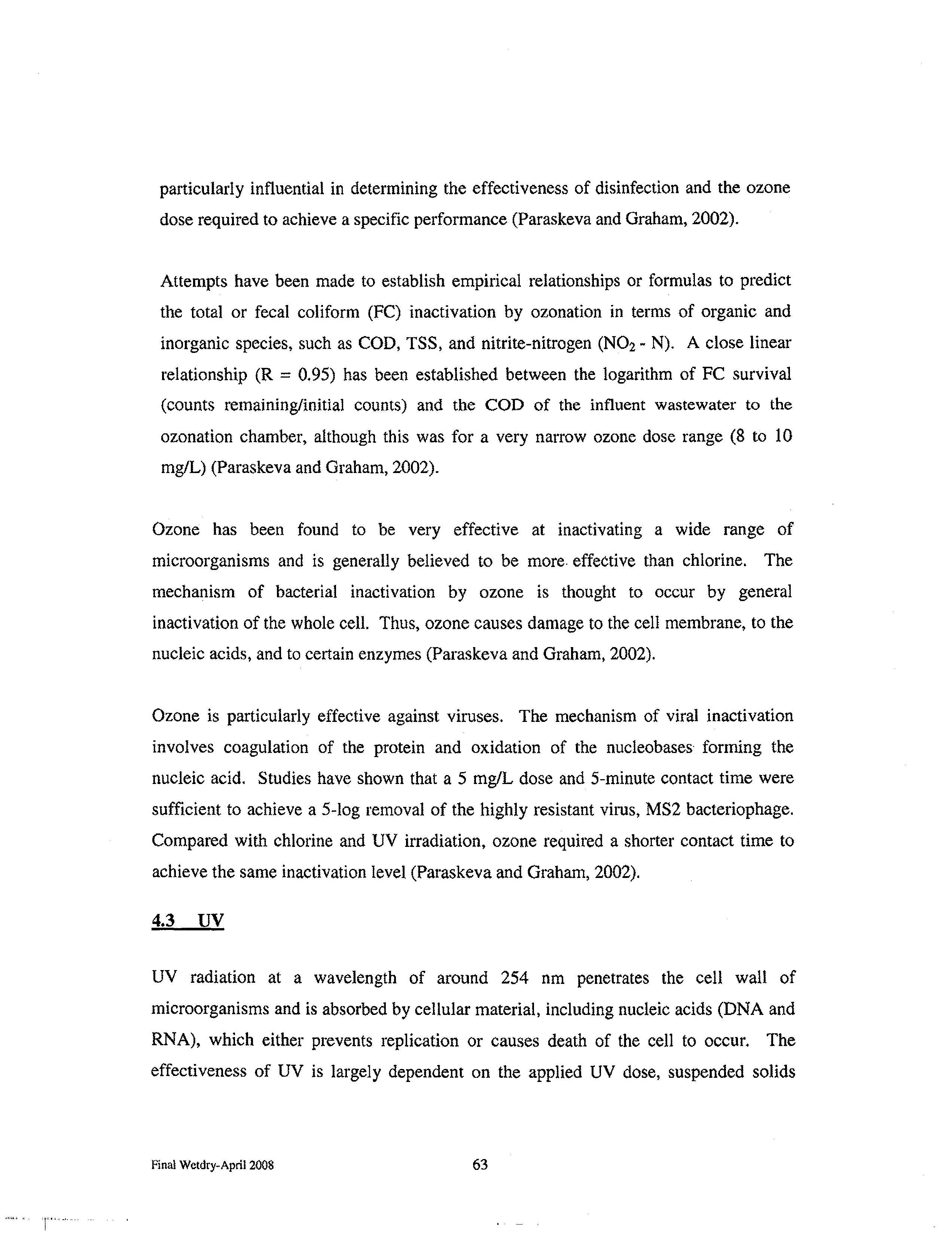
4.3
UV .................. ................................................................................................... 63
4.4
DISINFECTION BY-PRODUCTS (DBPS) AND RESIDUALS ..................................... 65
4.4.1
Chlorination DBPs and Residuals .............................................................67
4.4.2
Ozonation DBPS and Residuals ................................................................. 69
4.5
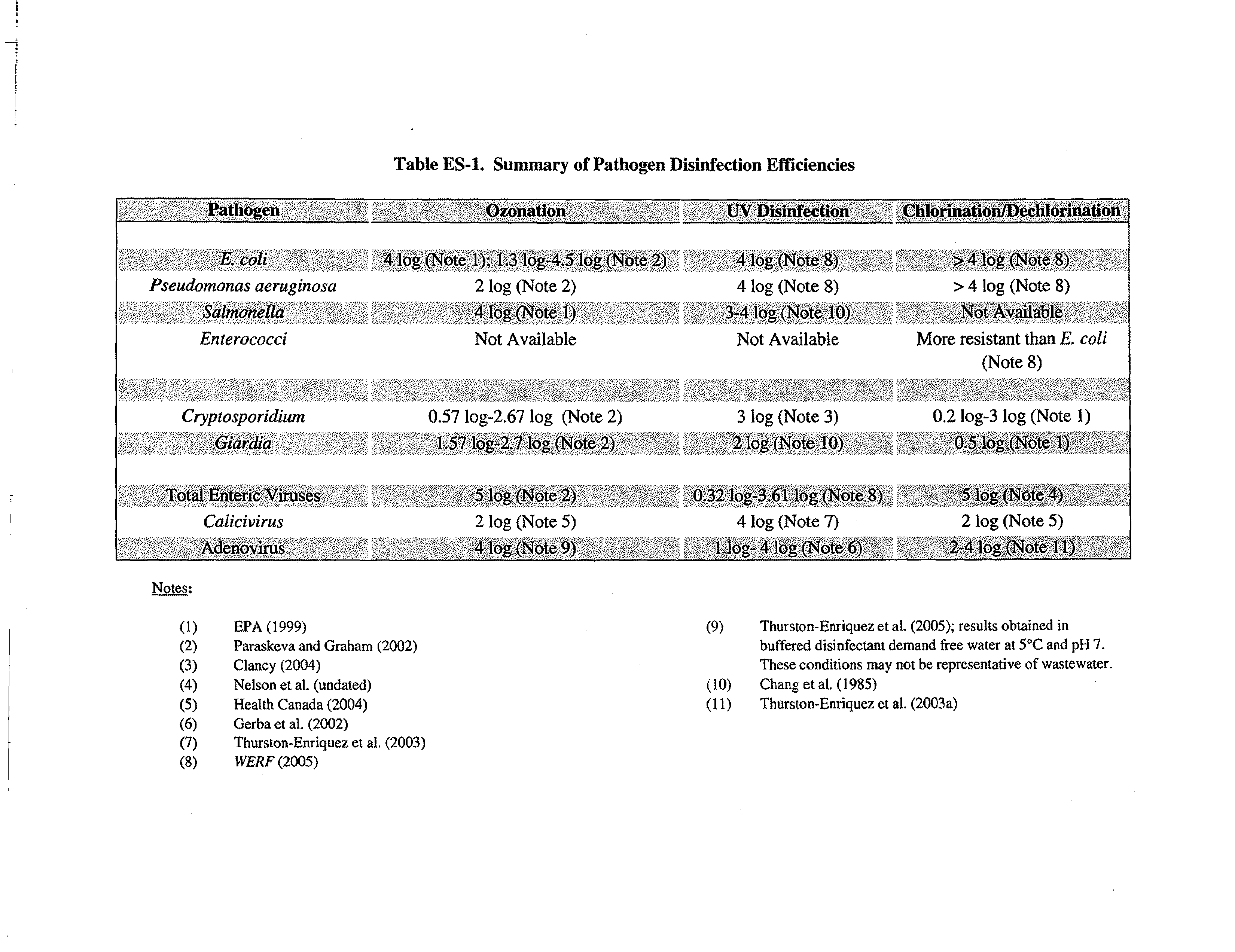
DISINFECTION EFFECTIVENESS ........................
...
........................................71
4.5.1
Bacteria Disinfection Efficiency ............................................................... 73
4.5.2
Protozoa Disinfection Efficiency .............................................................. 77
4.5.3
Virus Disinfection Efficiency ....................................................................81
4.6
SUMMARY AND CONCLUSIONS ........................................................................... 86
4.7
REFERENCES ...................................................................................................... 91
5.0
MICROBIAL RISK
ASSESSEMENT ..............................................................94
5.1
HAZARD IDENTIFICATION ...................................................................................94
5.2
EXPOSURE ASSESSMENT .................................................................................... 95
5.2.1
Waterway Use Summary and Receptor Group Categorization ................. 97
5.2.2
Exposure Inputs ........................................................................................ 99
5.3
DOSE-RESPONSE ASSESSMENT ......................................................................... 102
5.3.1
Enteric viruses .........................................................................................104
5.3.2
Calicivirus ...............................................................................................106
5.3.3
Adenovirus ..............................................................................................107
5.3.4
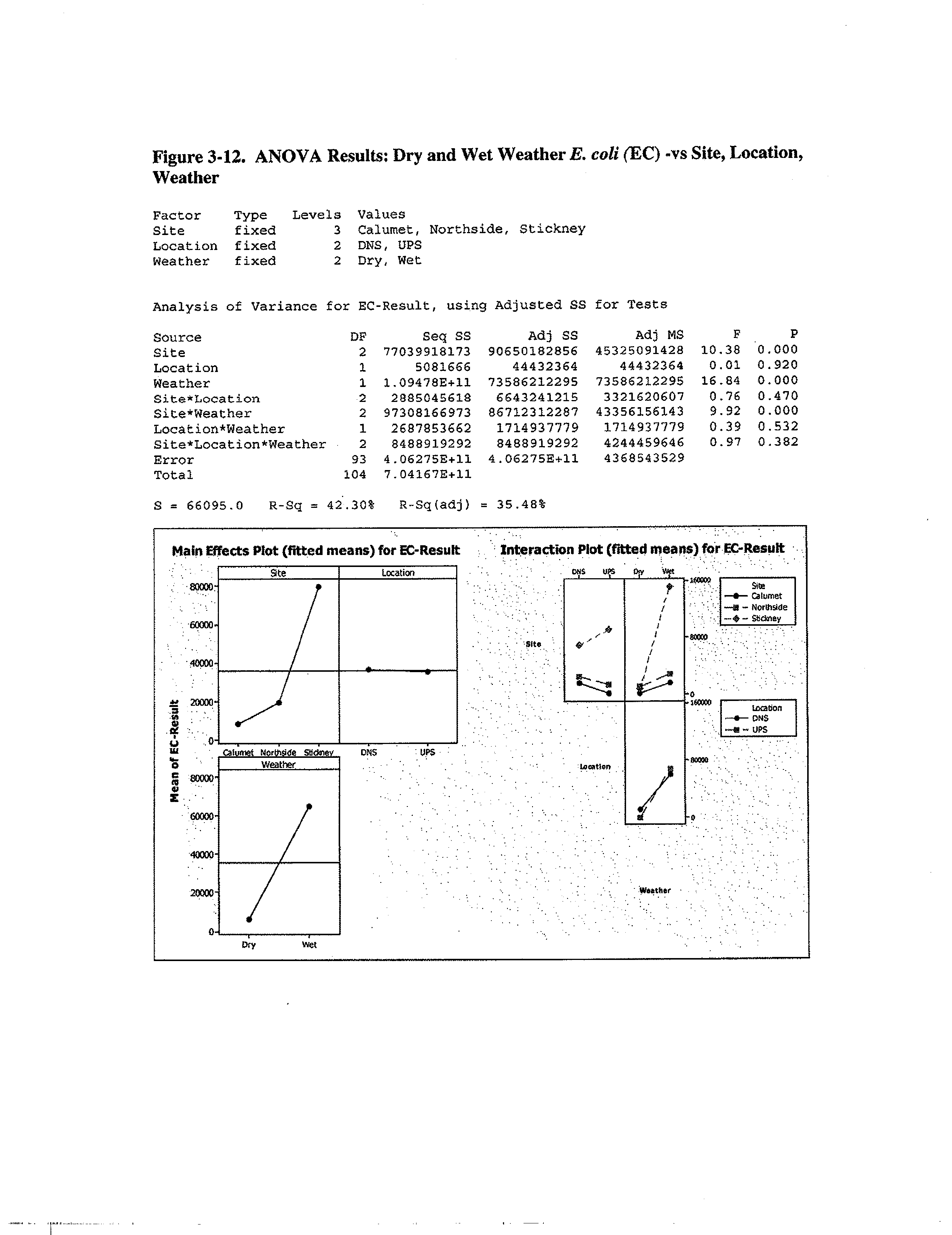
Escherichia coli .......................................................................................108
5.3.5
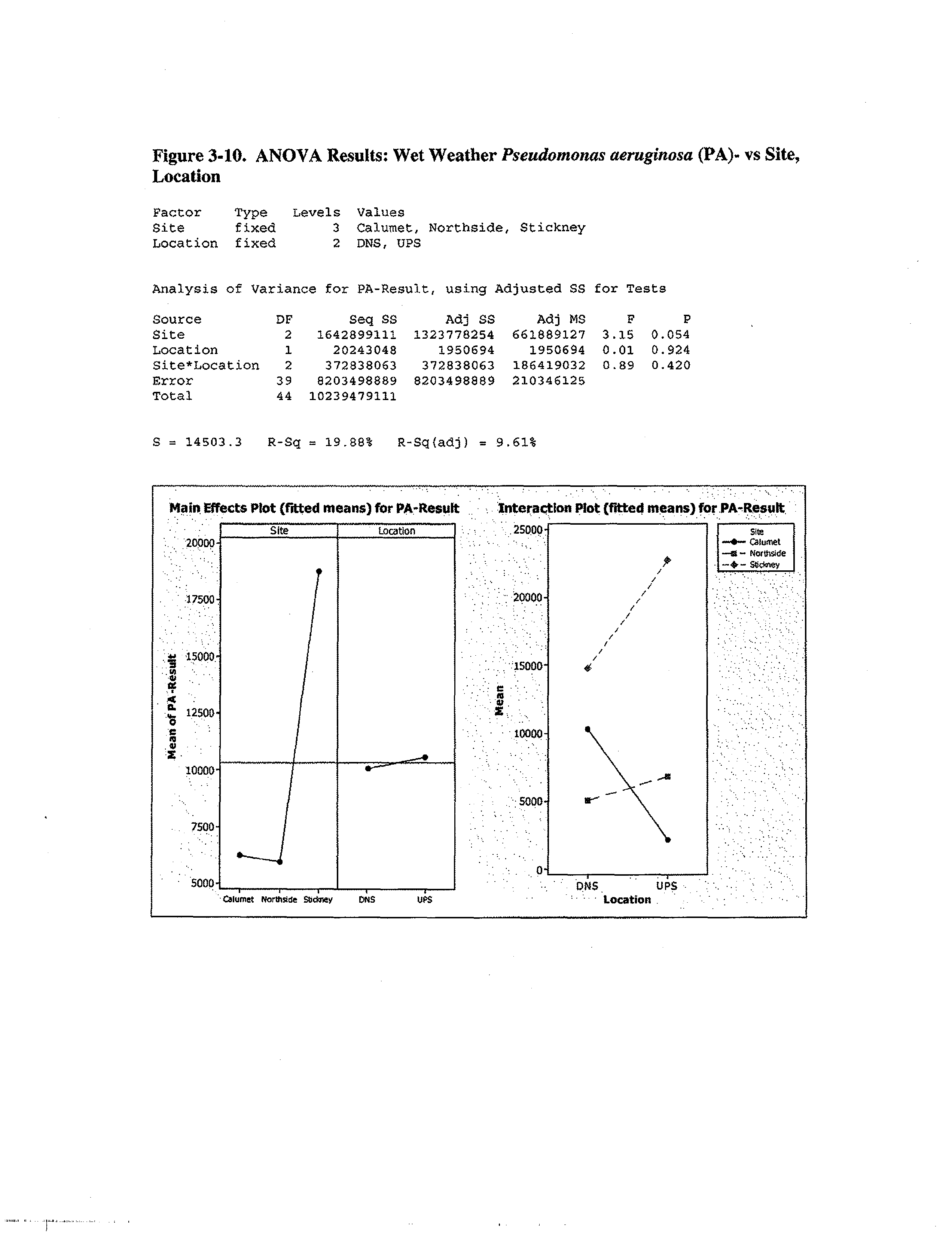
Pseudomonas aeruginosa ........................................................................
110
5.3.6
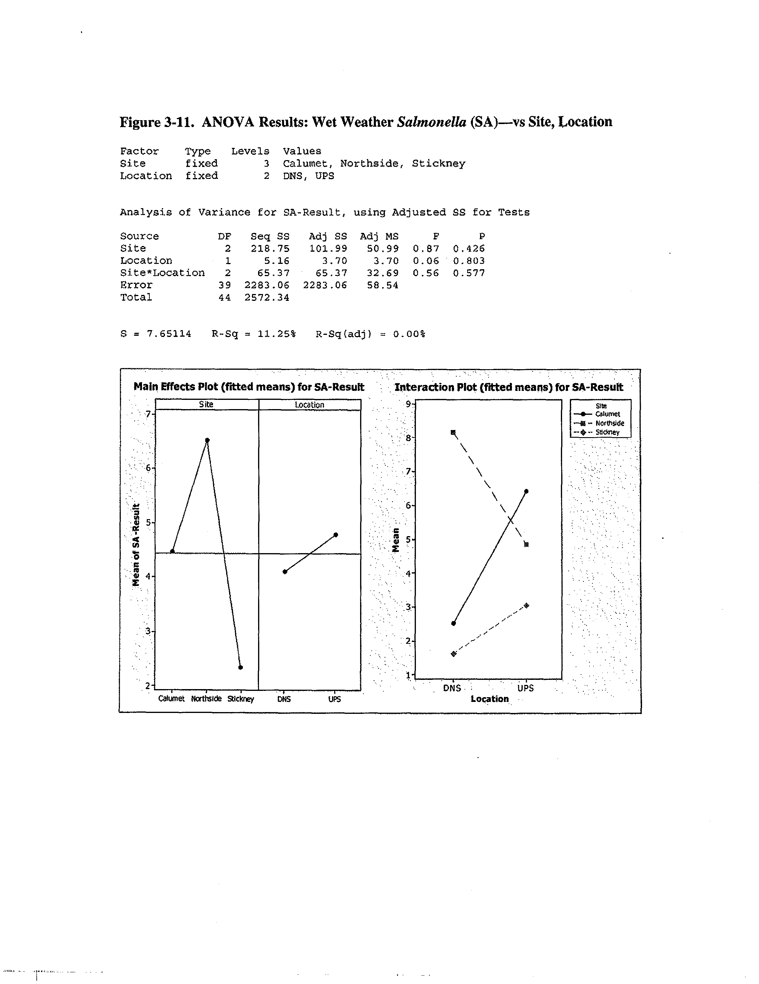
Salmonella ...............................................................................................112
5.3.7
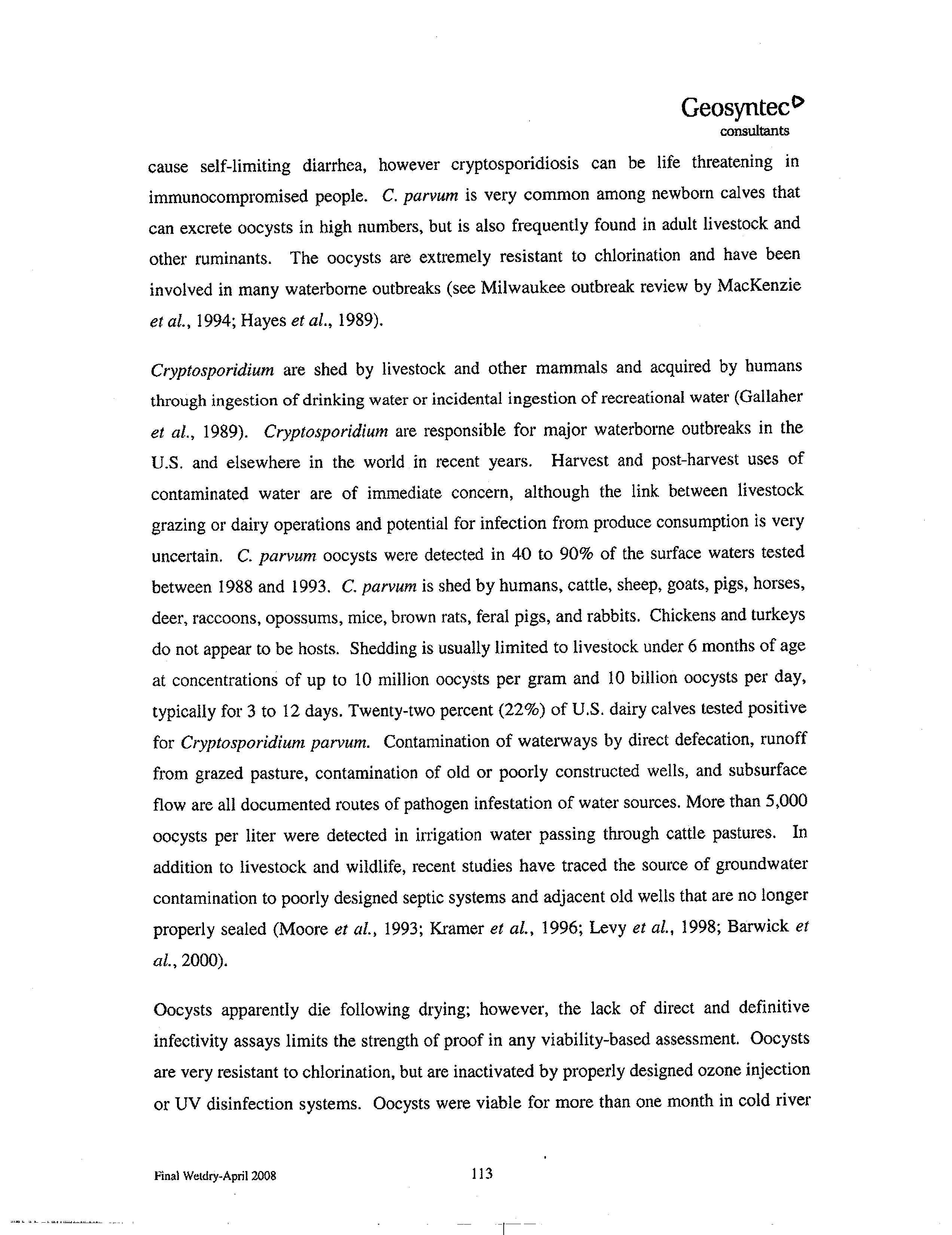
Cryptosporidium ......................................................................................112
5.3.8
Giardia
....................................................................................................114
5.4
RISK CHARACTERIZATION................................................................................. 115
Final Wetdry-April 2008
ii
TABLE OF CONTENTS
(Continued)
5.4.1
Probabilistic Analysis
..............................................................................
116
5.4.2
Disease Transmission Model ..................................................................120
5.4.3
Microbial Exposure Point Concentrations
..............................................121
5.4.4
Weather
...................................................................................................124
5.4.5
Simulations
..............................................................................................125
5.4.6
Risk Assessment Calculation Results and Conclusions
..........................126
5.4.7
Sensitivity and Uncertainty Analysis ...................................................... 130
5.5
REFERENCES
......................................... ...........................................................
133
Final
Wetdry-April 2008
iii
Geosynte&
consultants
LIST OF TABLES
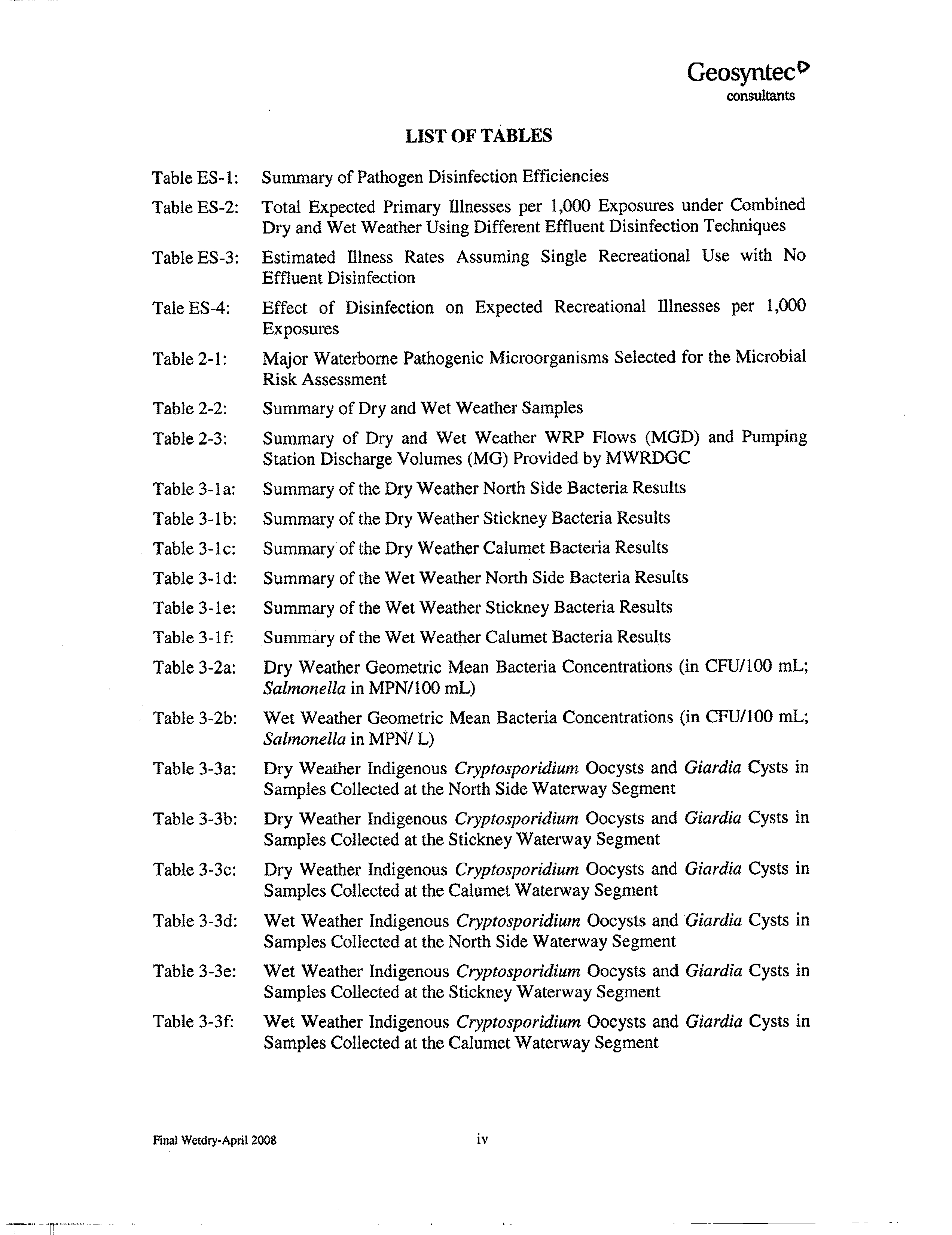
Table ES-1:
Summary of Pathogen Disinfection Efficiencies
Table ES-2:
Total Expected Primary Illnesses
per
1,000 Exposures under Combined
Dry and Wet Weather Using Different Effluent Disinfection Techniques
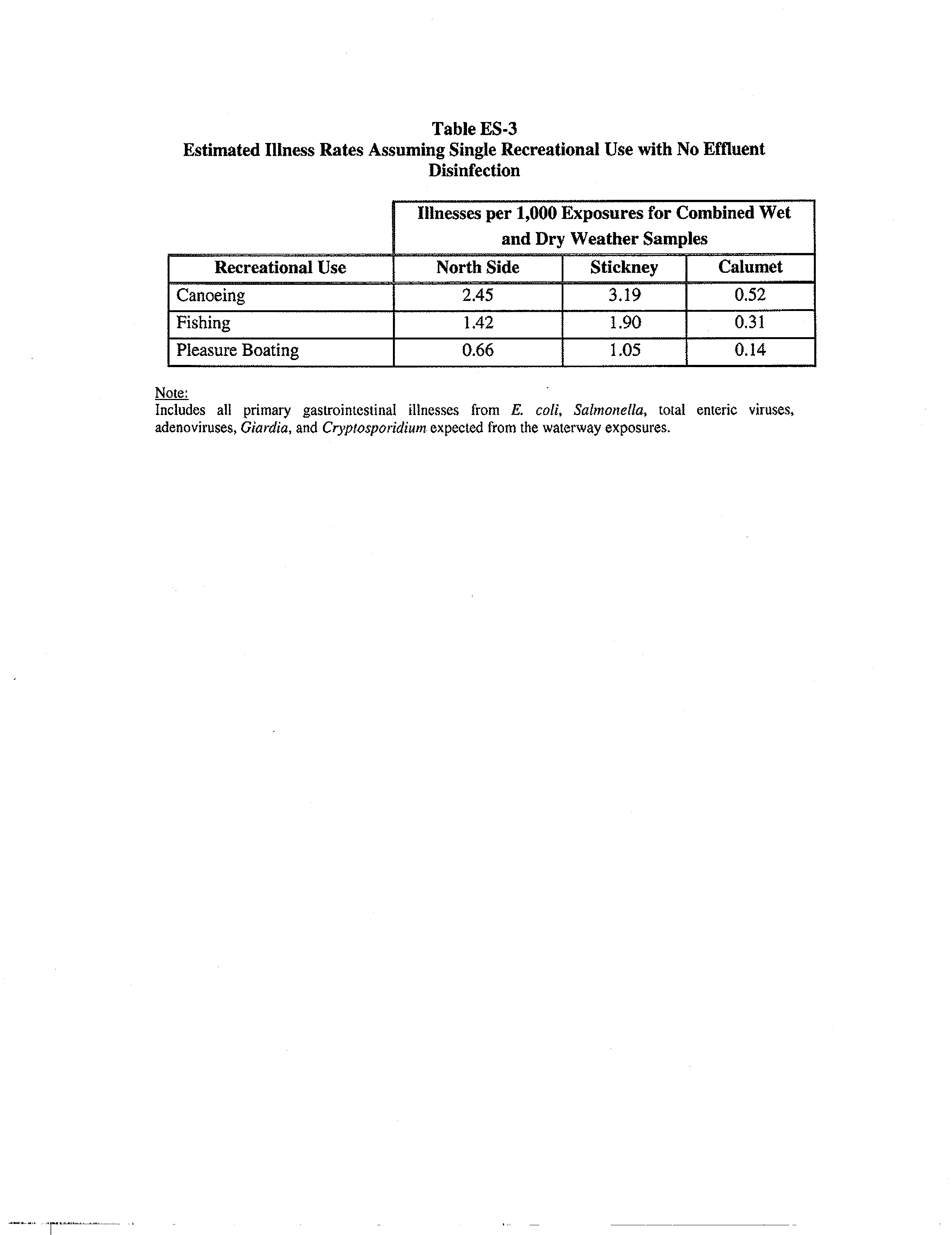
Table ES-3:
Estimated Illness Rates Assuming Single Recreational Use with No
Effluent Disinfection
Tale ES-4:
Effect of Disinfection on Expected Recreational Illnesses per 1,000
Exposures
Table 2-1:
Major Waterborne Pathogenic Microorganisms Selected for the Microbial
Risk Assessment
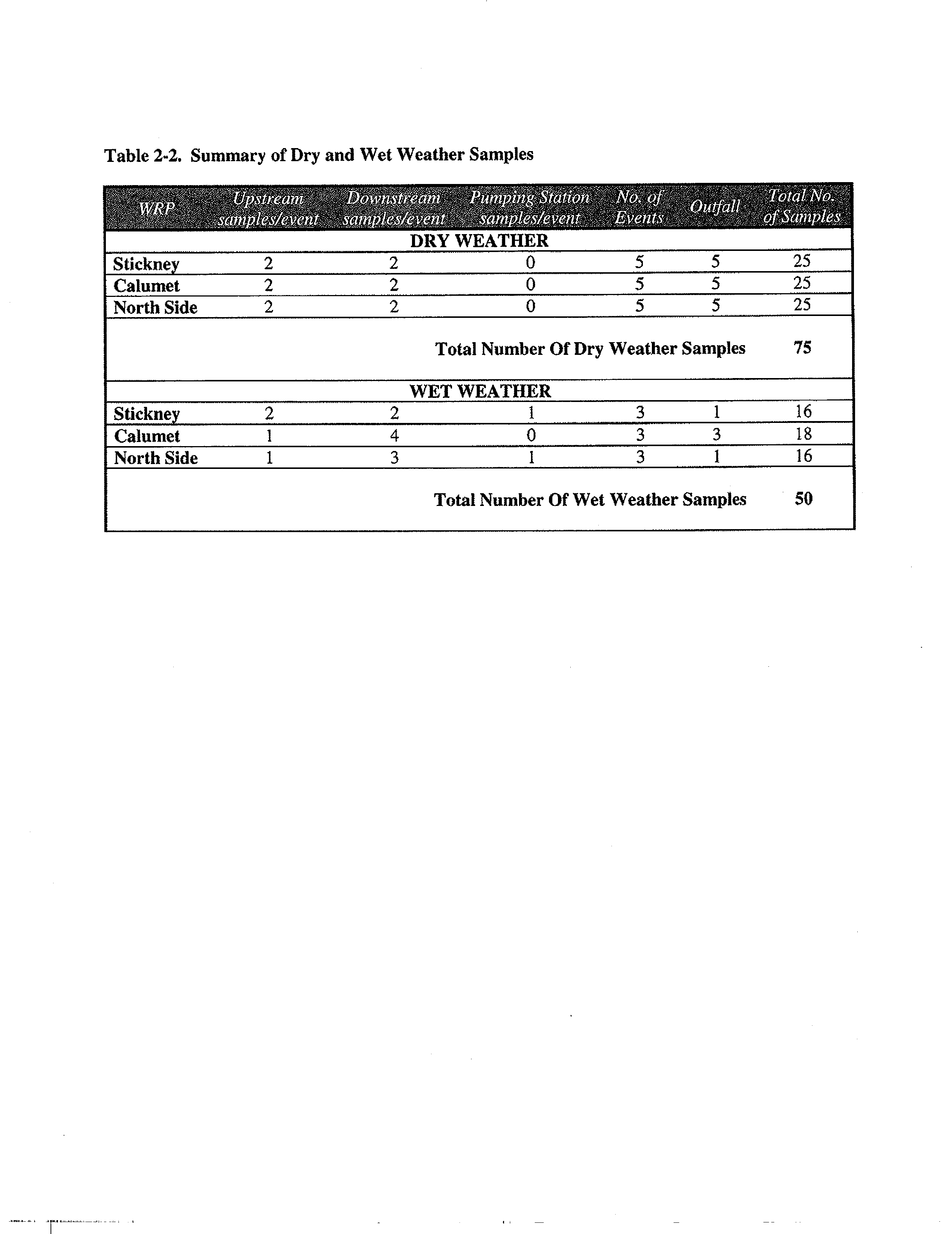
Table 2-2:
Summary of Dry and Wet Weather Samples
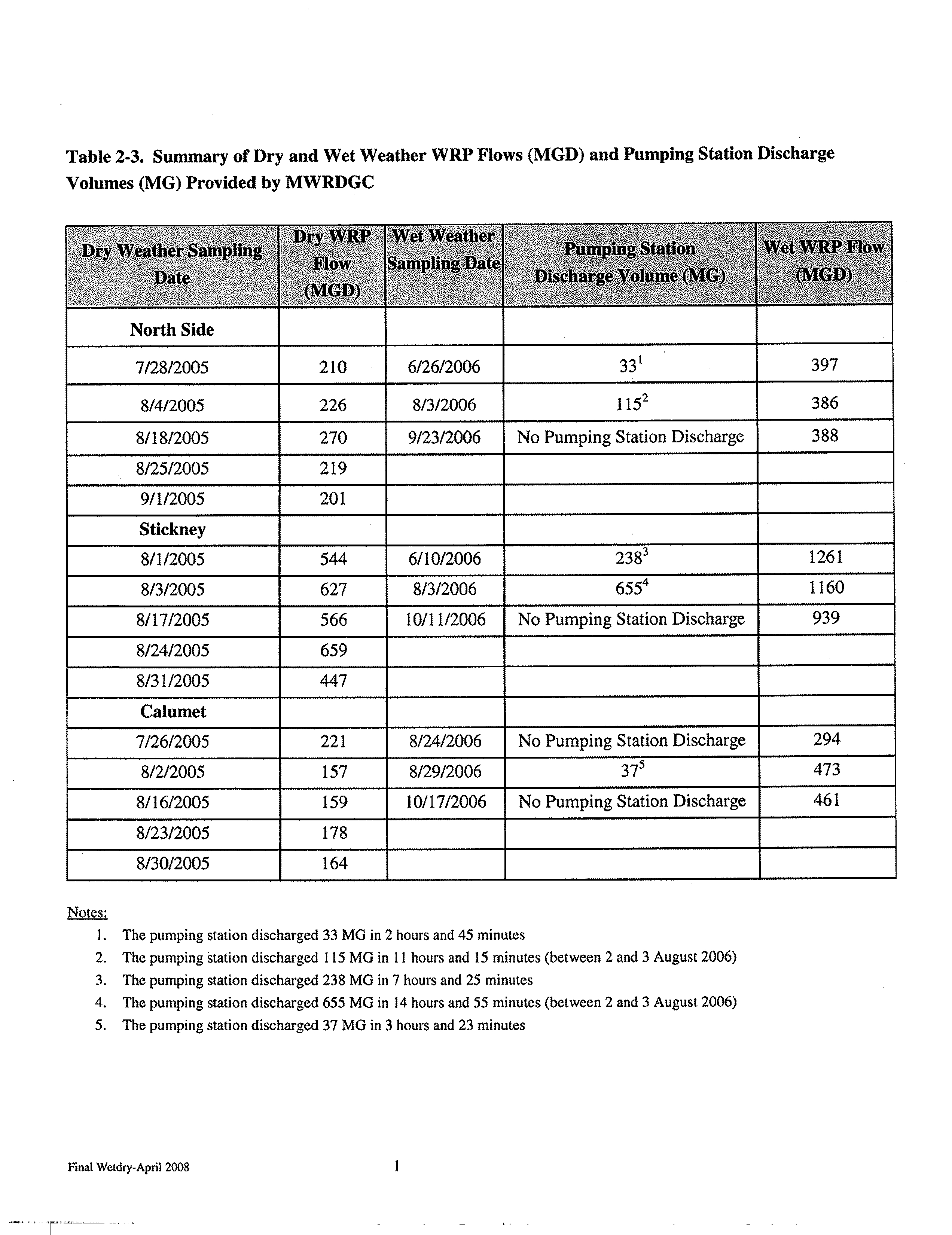
Table 2-3:
Summary of Dry and Wet Weather WRP Flows (MGD) and Pumping
Station Discharge Volumes (MG) Provided by MWRDGC
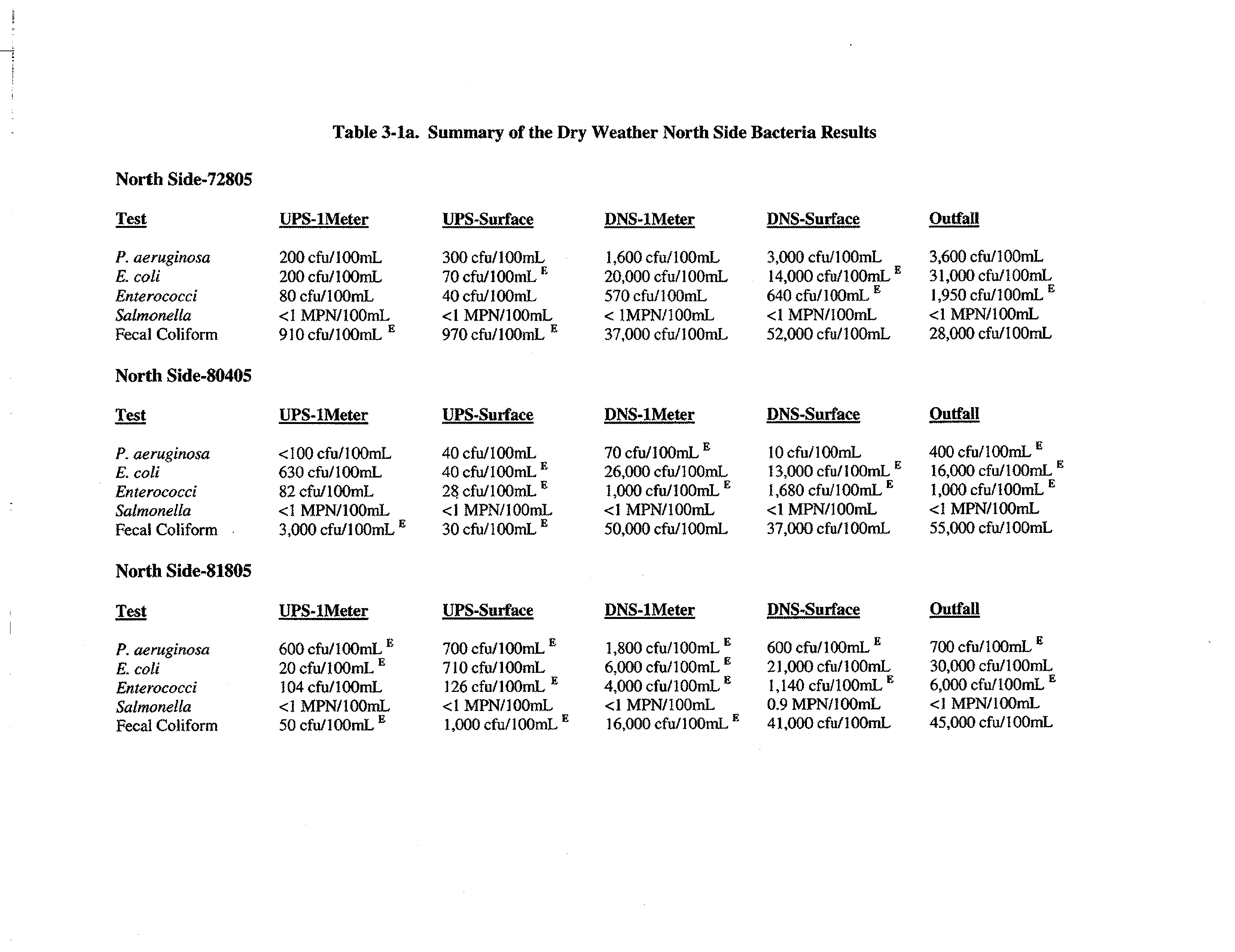
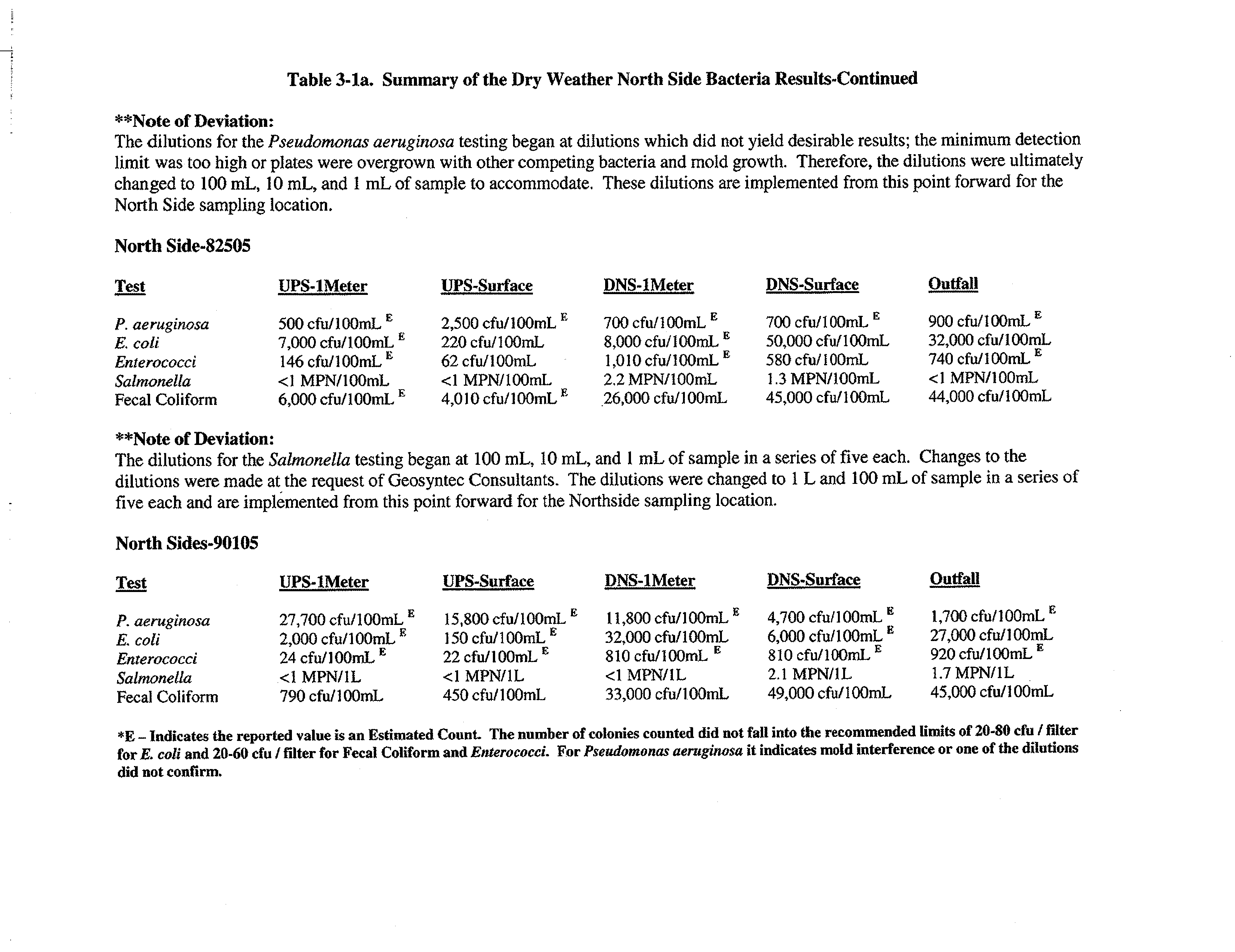
Table 3-1a:
Summary of the Dry Weather North Side Bacteria Results
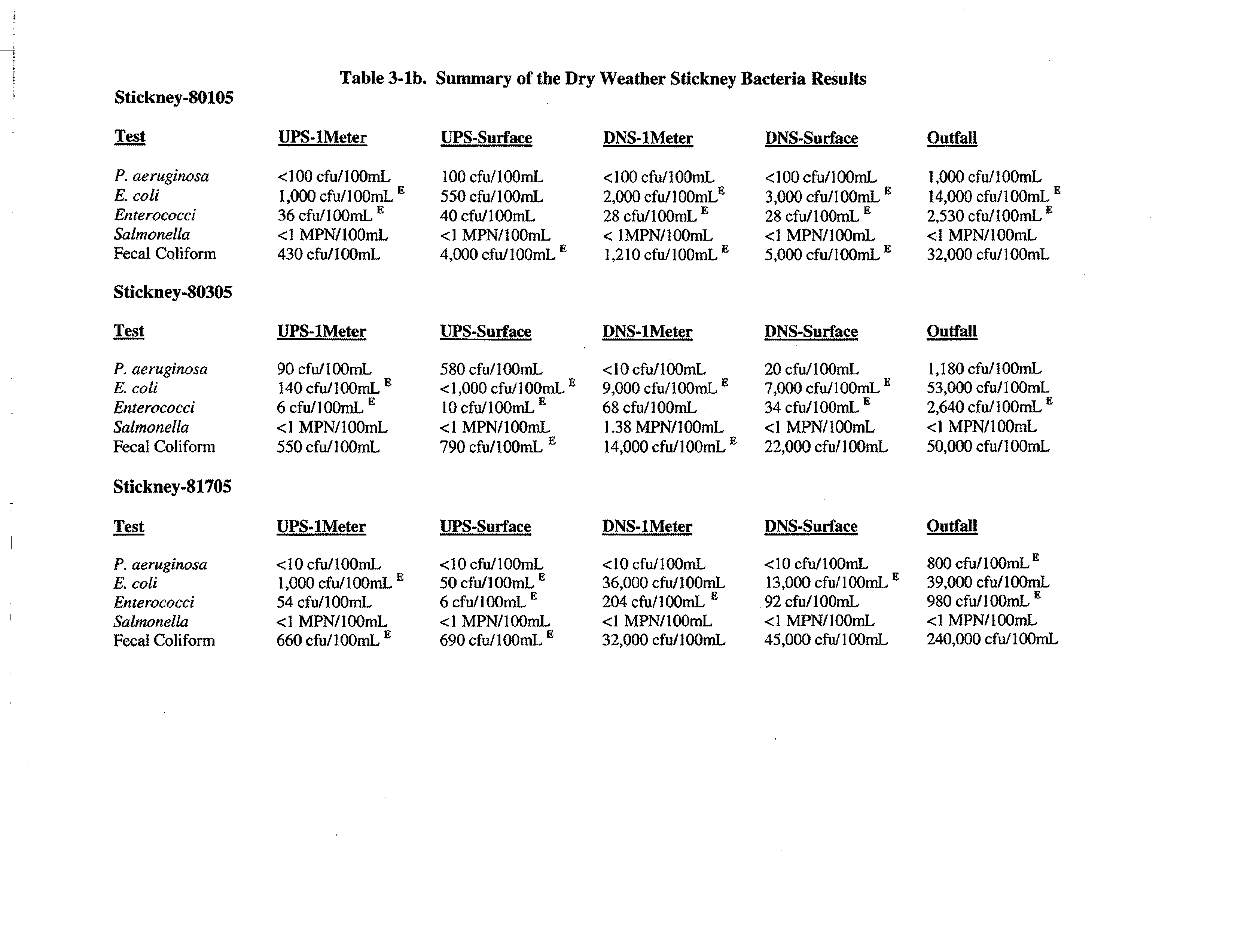
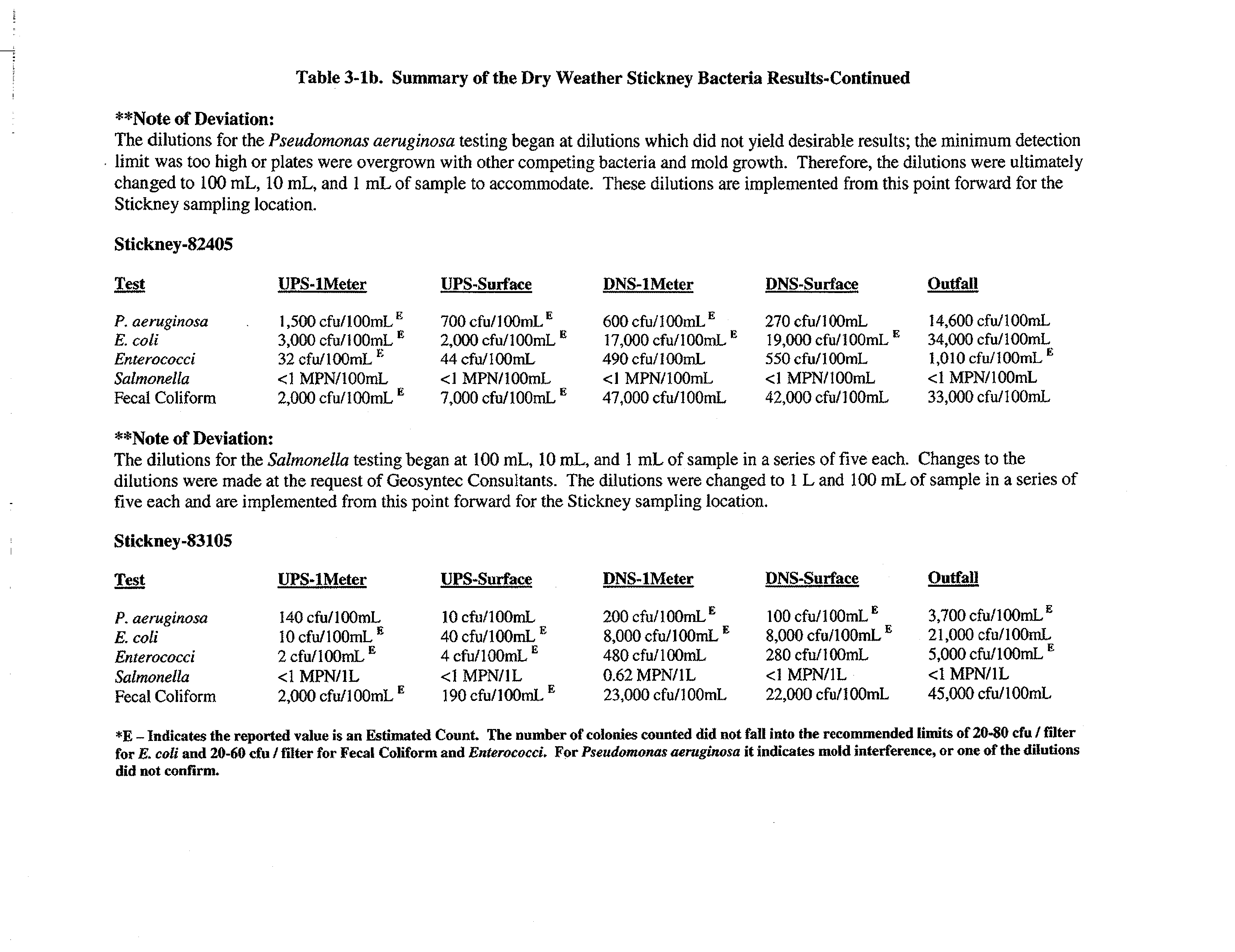
Table 3-1 b:
Summary of the Dry Weather Stickney Bacteria Results
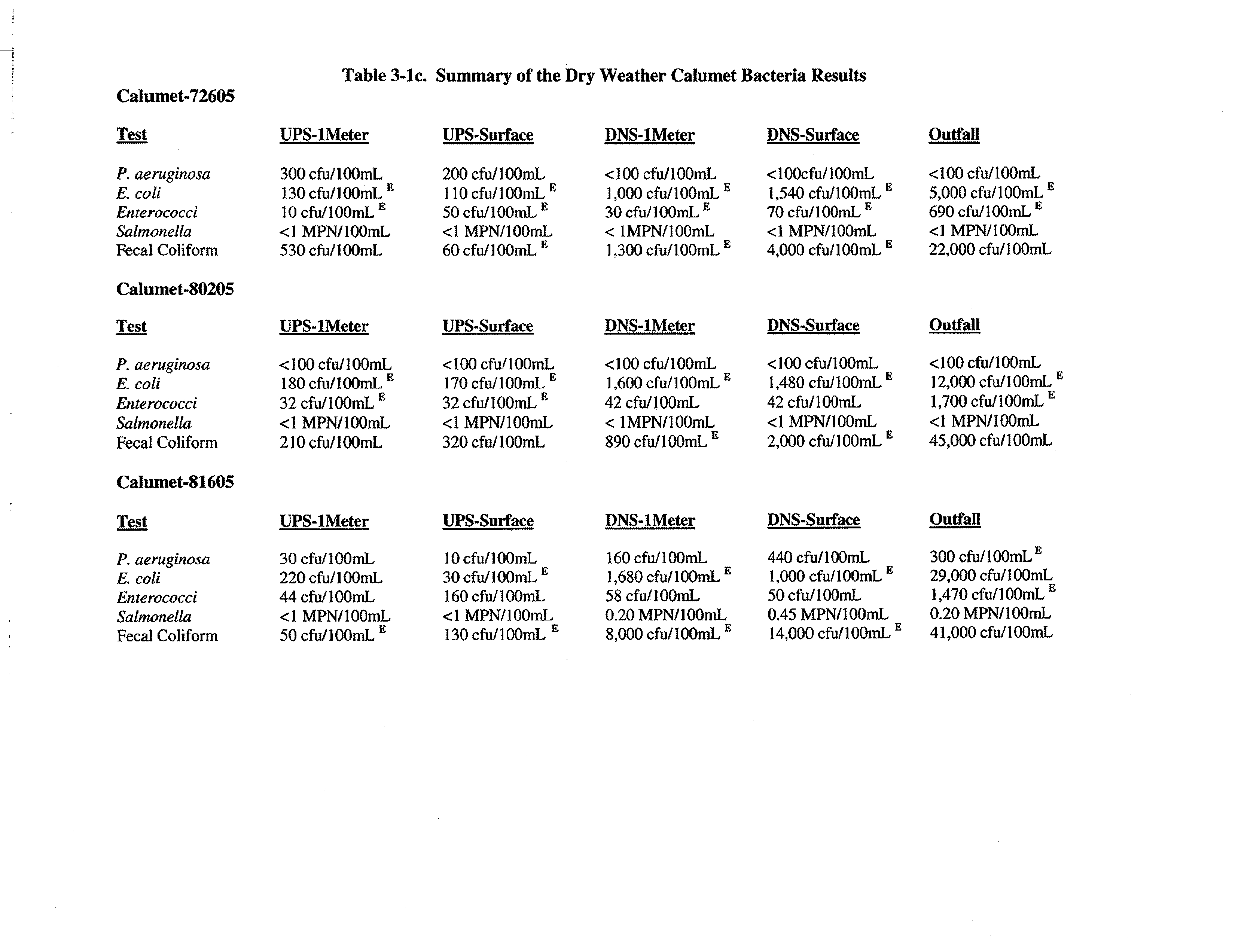
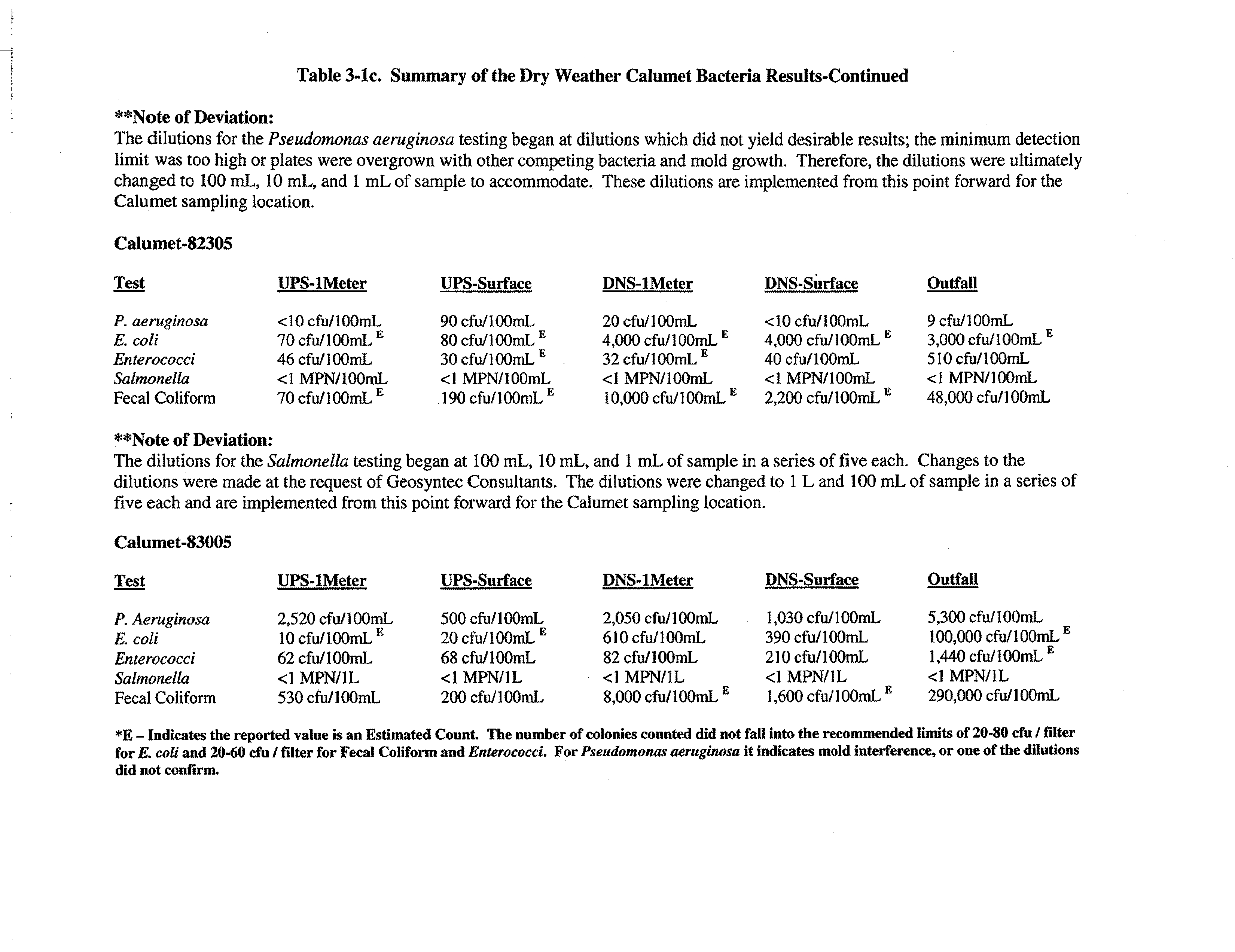
Table 3-1c:
Summary of the Dry Weather Calumet Bacteria Results
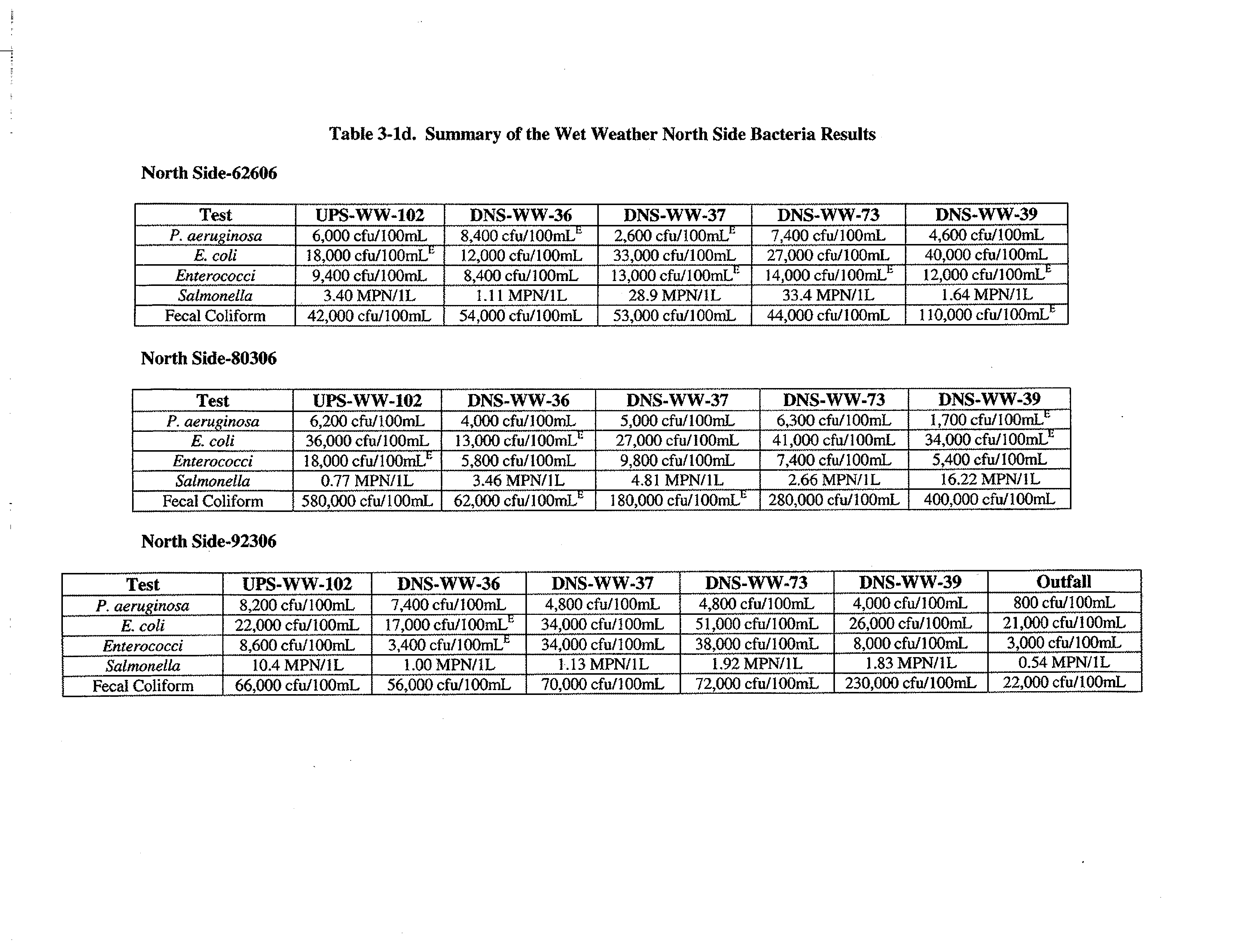
Table 3-1 d:
Summary of the Wet Weather North Side Bacteria Results
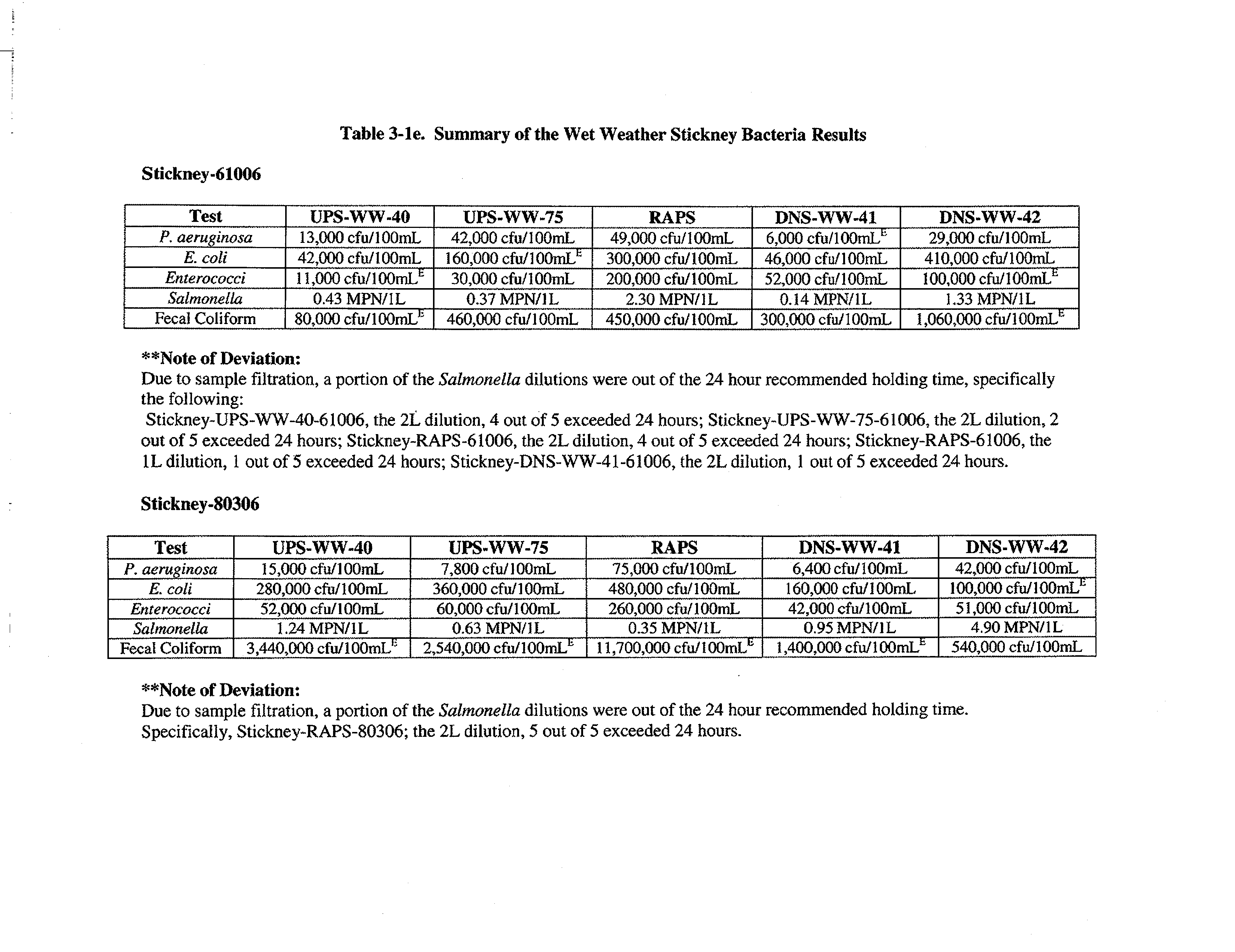
Table 3-le:
Summary of the Wet Weather Stickney Bacteria Results
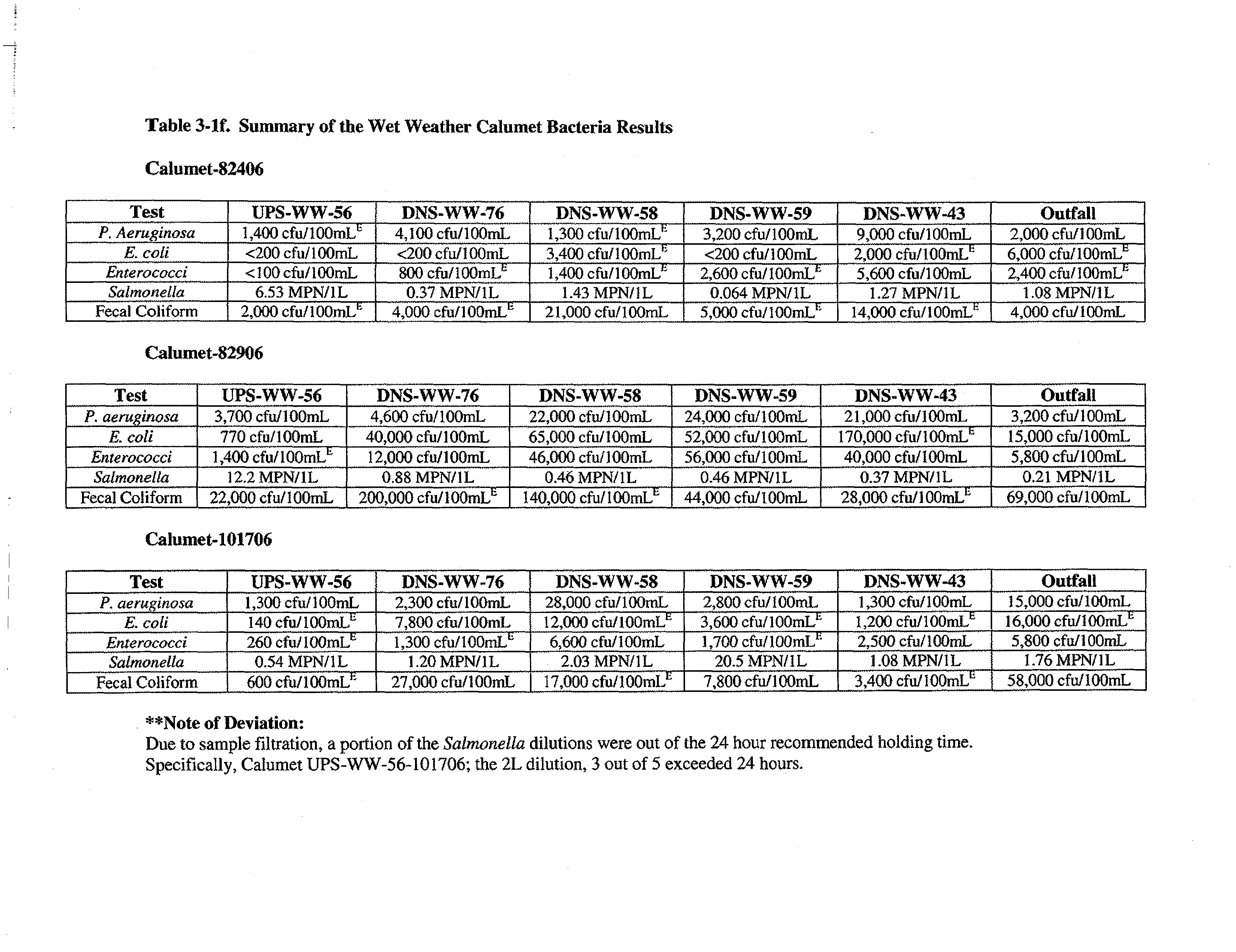
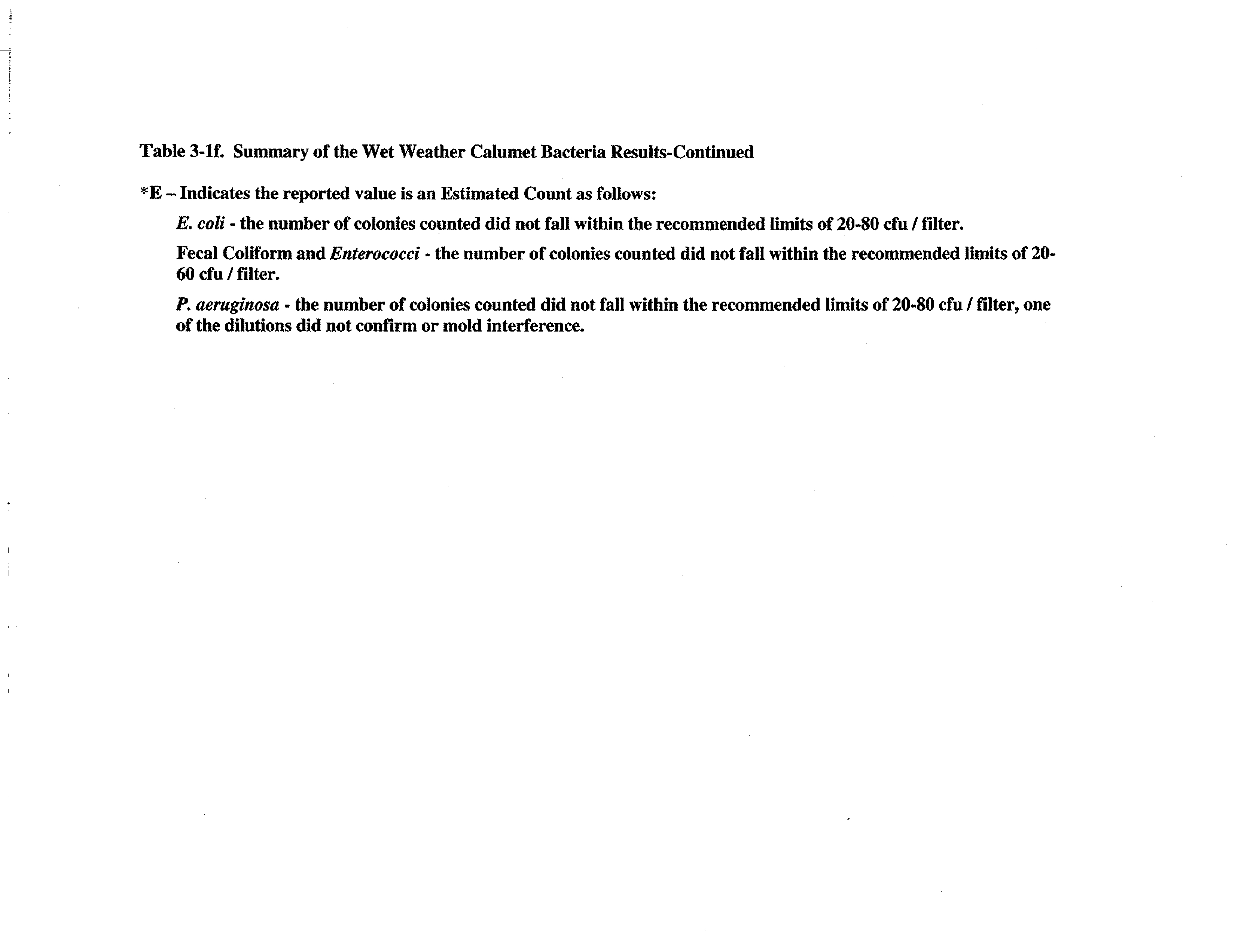
Table 3-1f:
Summary of the Wet Weather Calumet Bacteria Results
Table 3-2a:
Dry Weather Geometric Mean Bacteria Concentrations {in CFU/100 mL;
Salmonella
in
MPN/100 mL)
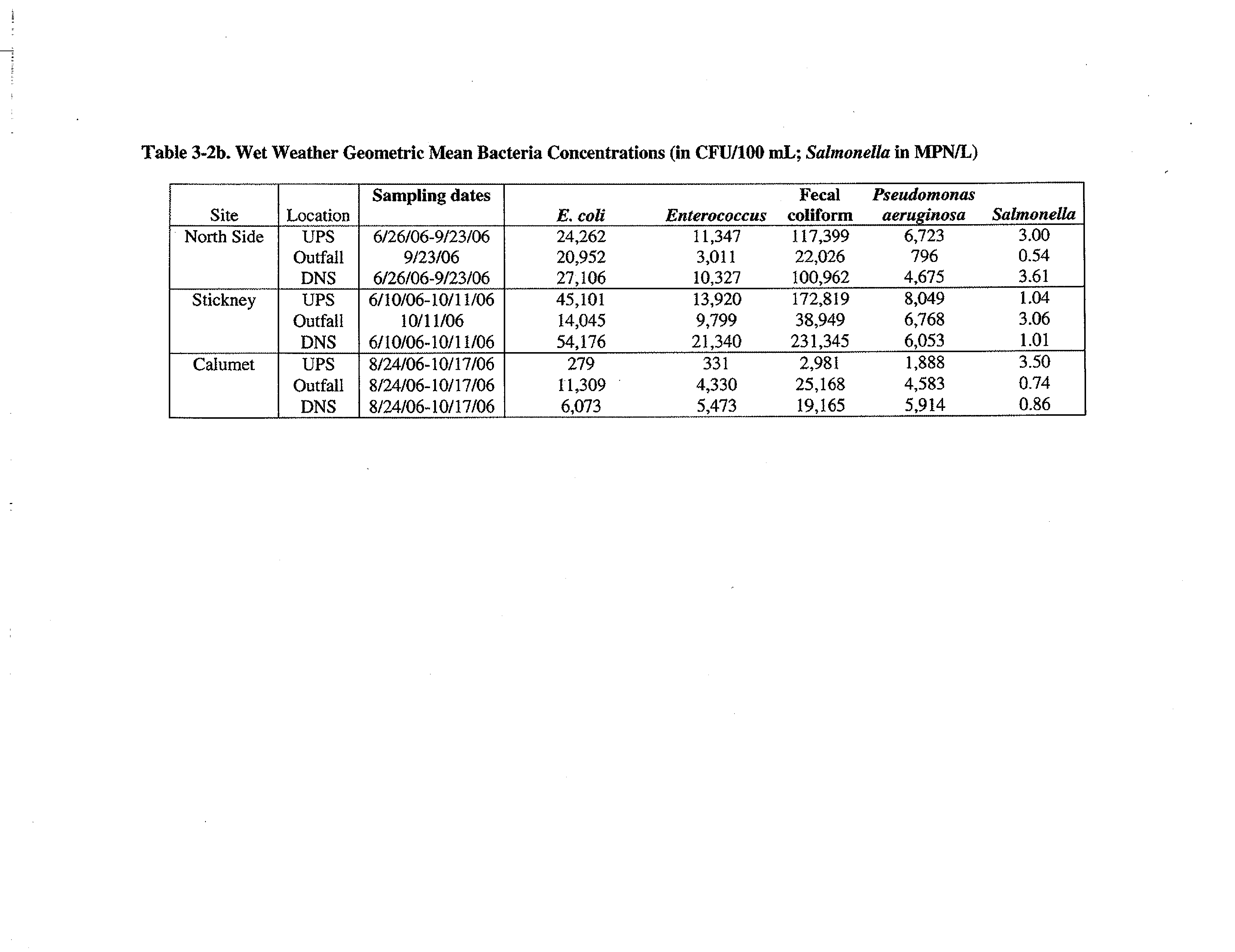
Table 3-2b:
Wet Weather Geometric Mean Bacteria Concentrations {in CFU/100 mL;
Salmonella
in MPN/ Q
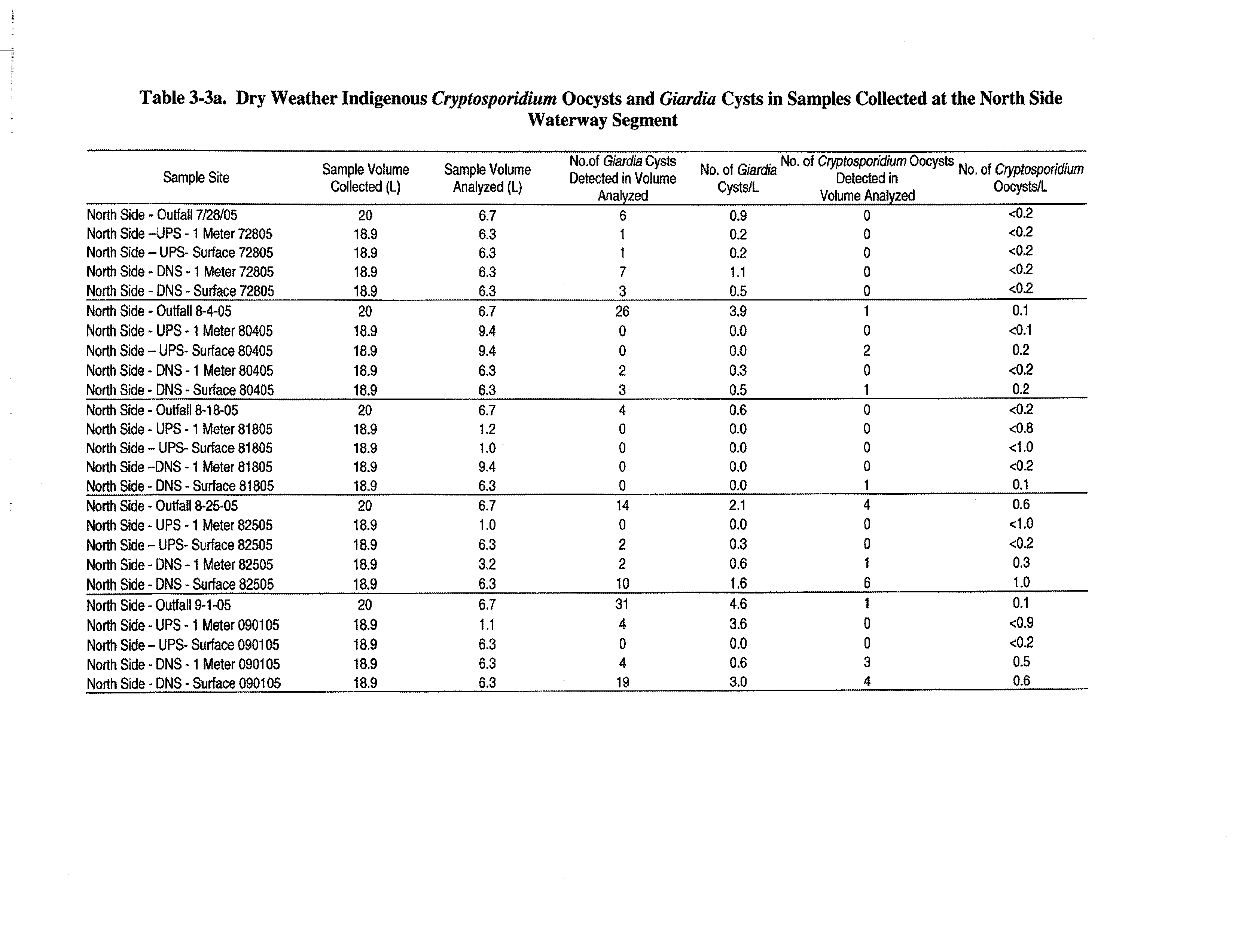
Table 3-3a:
Dry Weather Indigenous
Cryptosporidium
Oocysts and
Giardia
Cysts in
Samples Collected at the North Side Waterway Segment
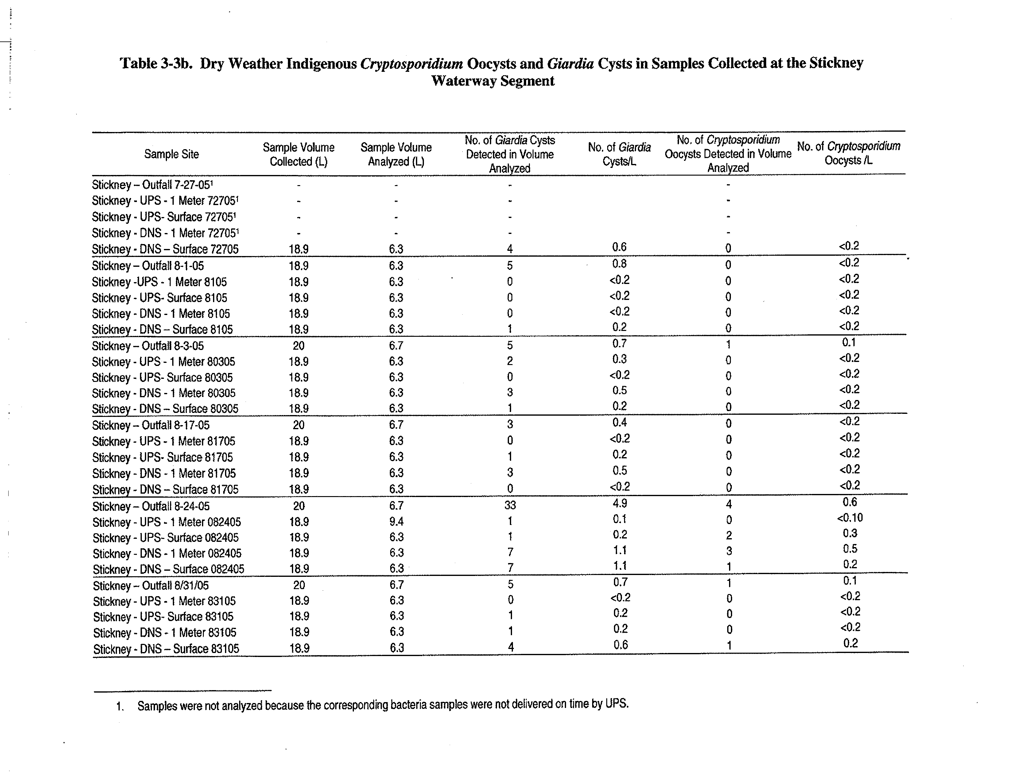
Table 3-3b:
Dry Weather Indigenous
Cryptosporidium
Oocysts and
Giardia
Cysts in
Samples Collected at the Stickney Waterway Segment
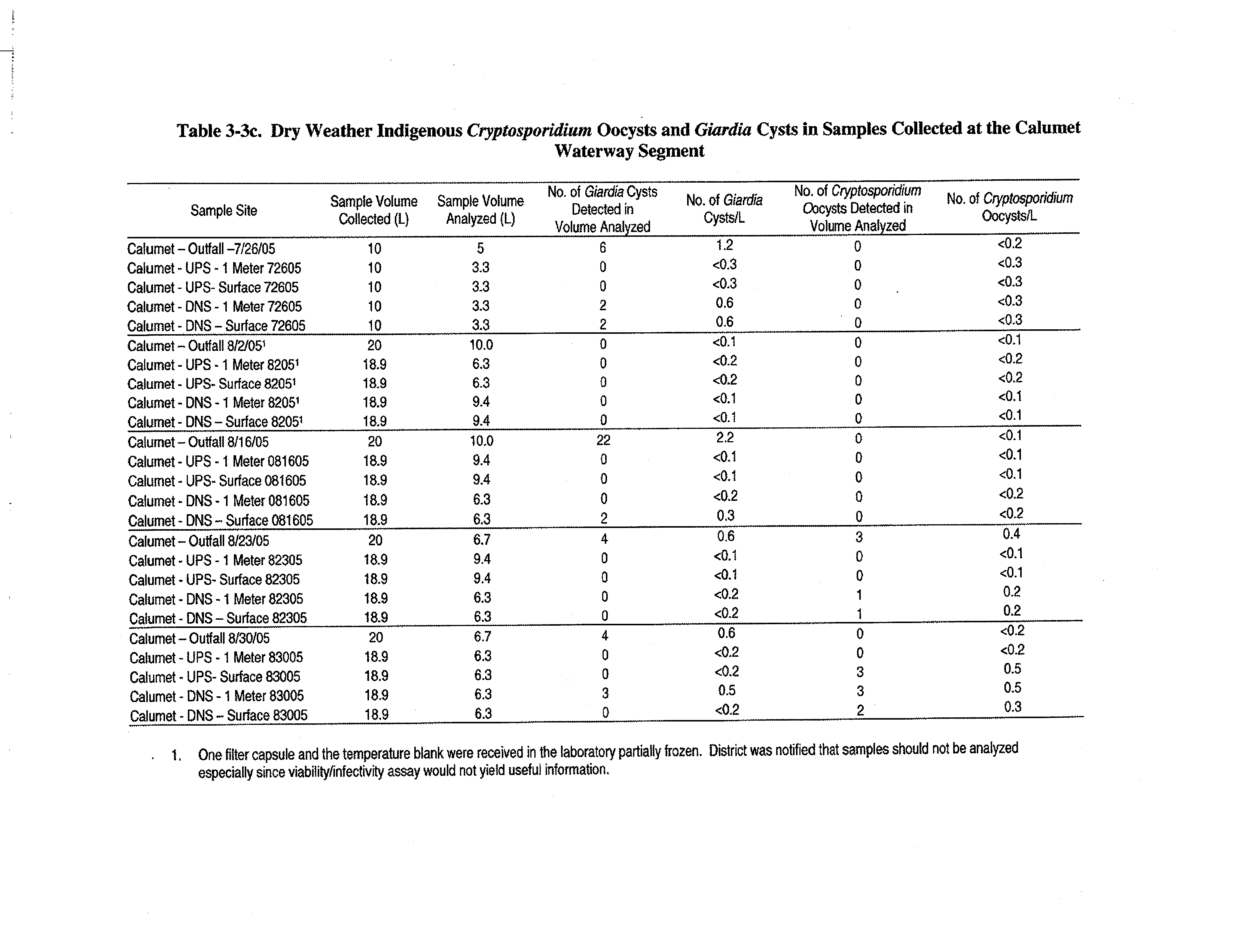
Table 3-3c:
Dry Weather Indigenous
Cryptosporidium
Oocysts and
Giardia
Cysts in
Samples Collected at the Calumet Waterway Segment
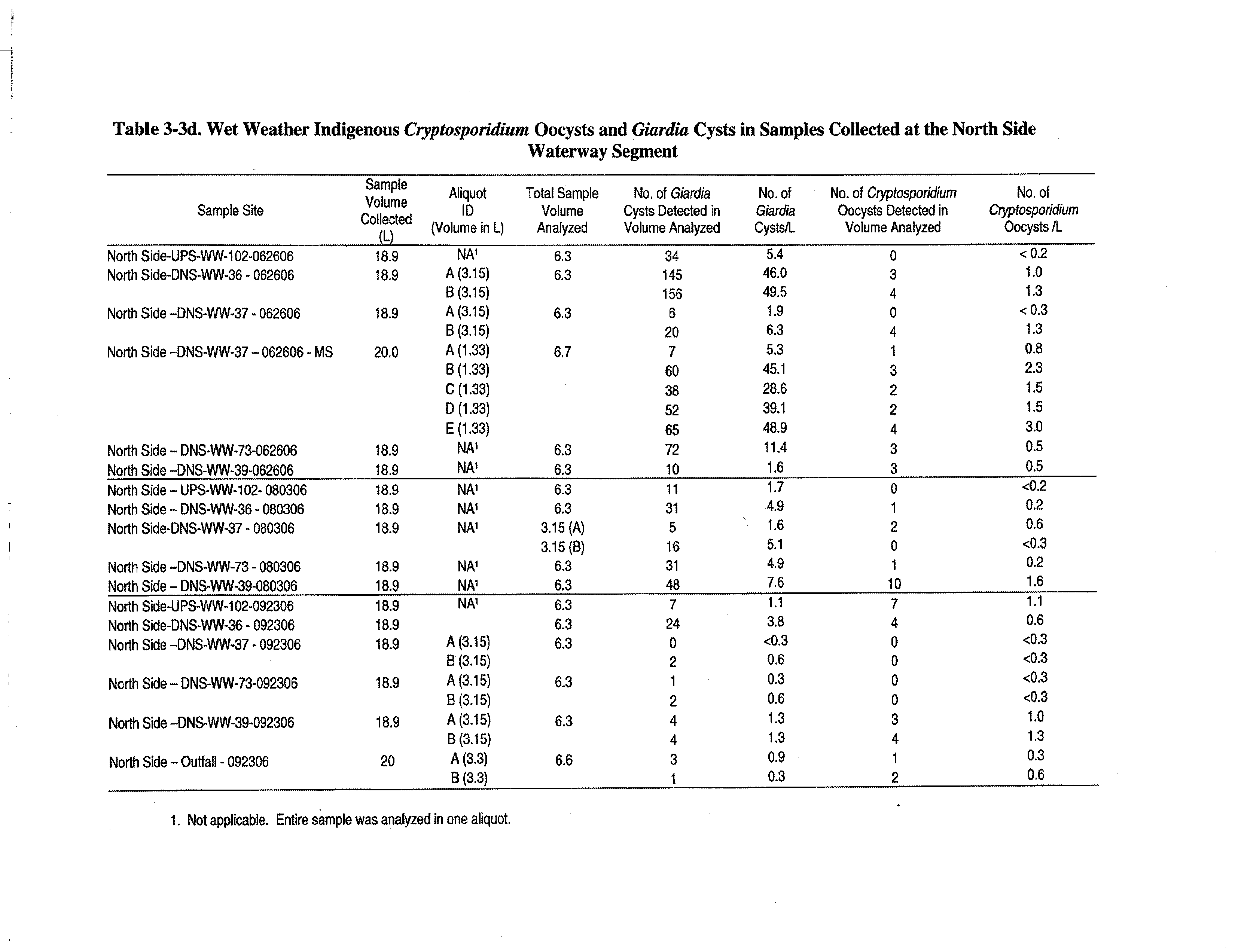
Table 3-3d:
Wet Weather Indigenous
Cryptosporidium
Oocysts and
Giardia
Cysts in
Samples Collected at the North Side Waterway Segment
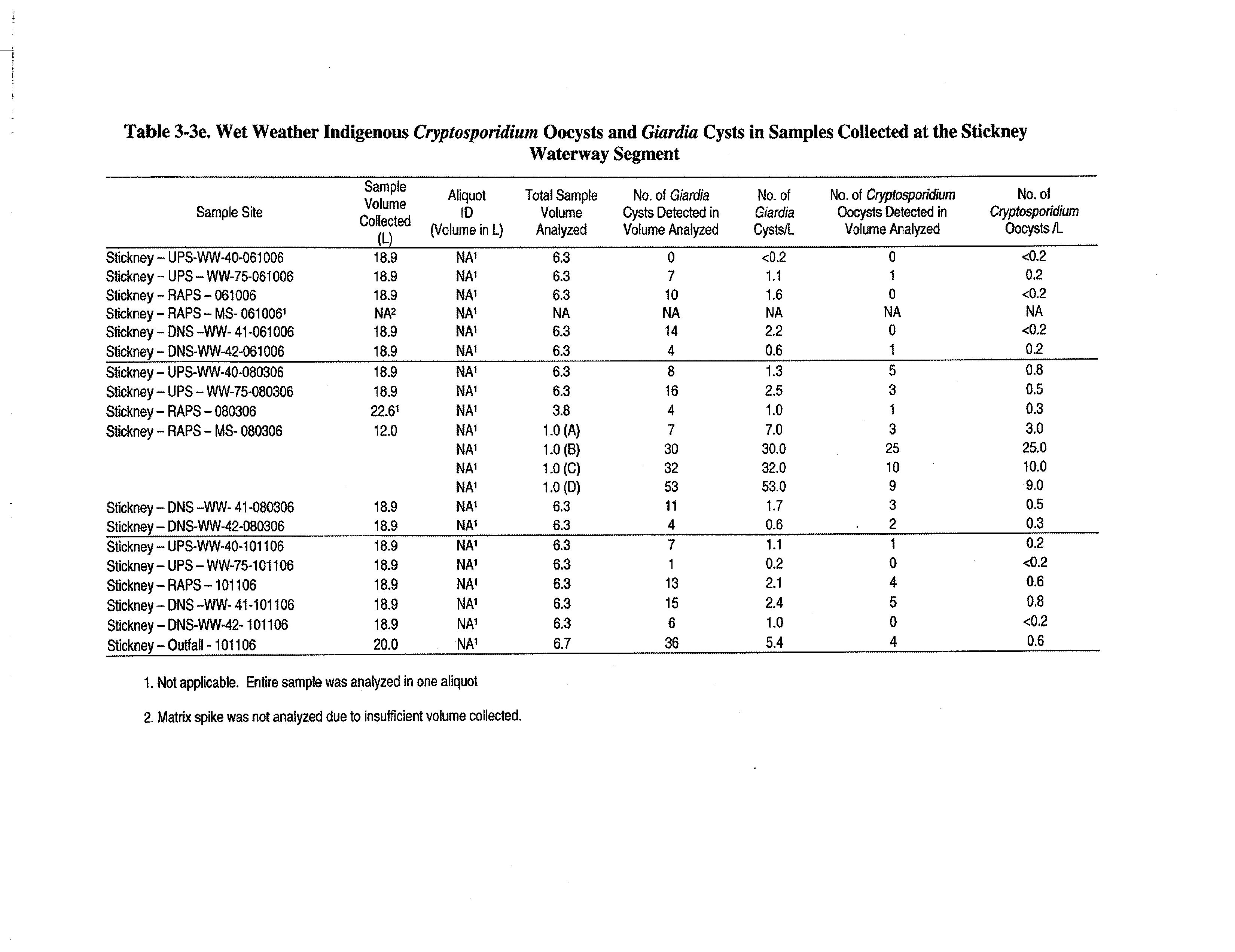
Table 3-3e:
Wet Weather Indigenous
Cryptosporidium
Oocysts and
Giardia
Cysts in
Samples Collected at the Stickney Waterway Segment
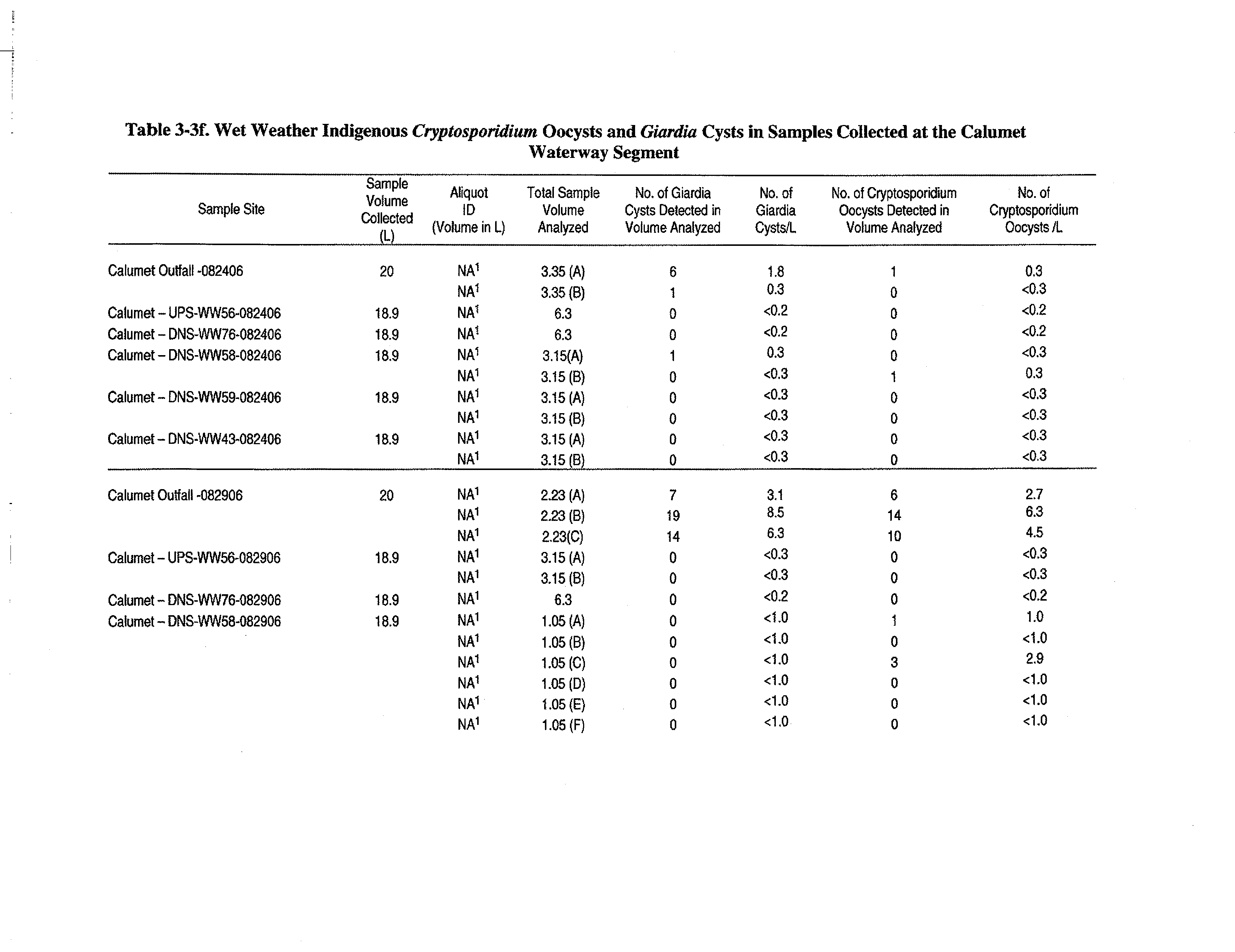
Table 3-3f:
Wet Weather Indigenous
Cryptosporidium
Oocysts and
Giardia
Cysts in
Samples Collected at the Calumet Waterway Segment
Final Wetdry-April 2009
iv
LIST OF TABLES (
Continued)
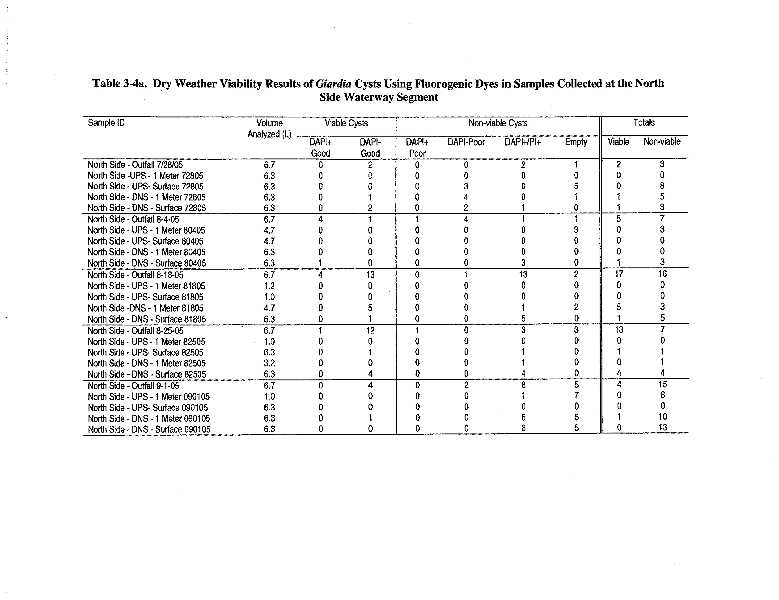
Table 3-4a:
Dry Weather Viability Results of
Giardia
Cysts Using Fluorogenic Dyes
in Samples Collected at the North Side Waterway Segment
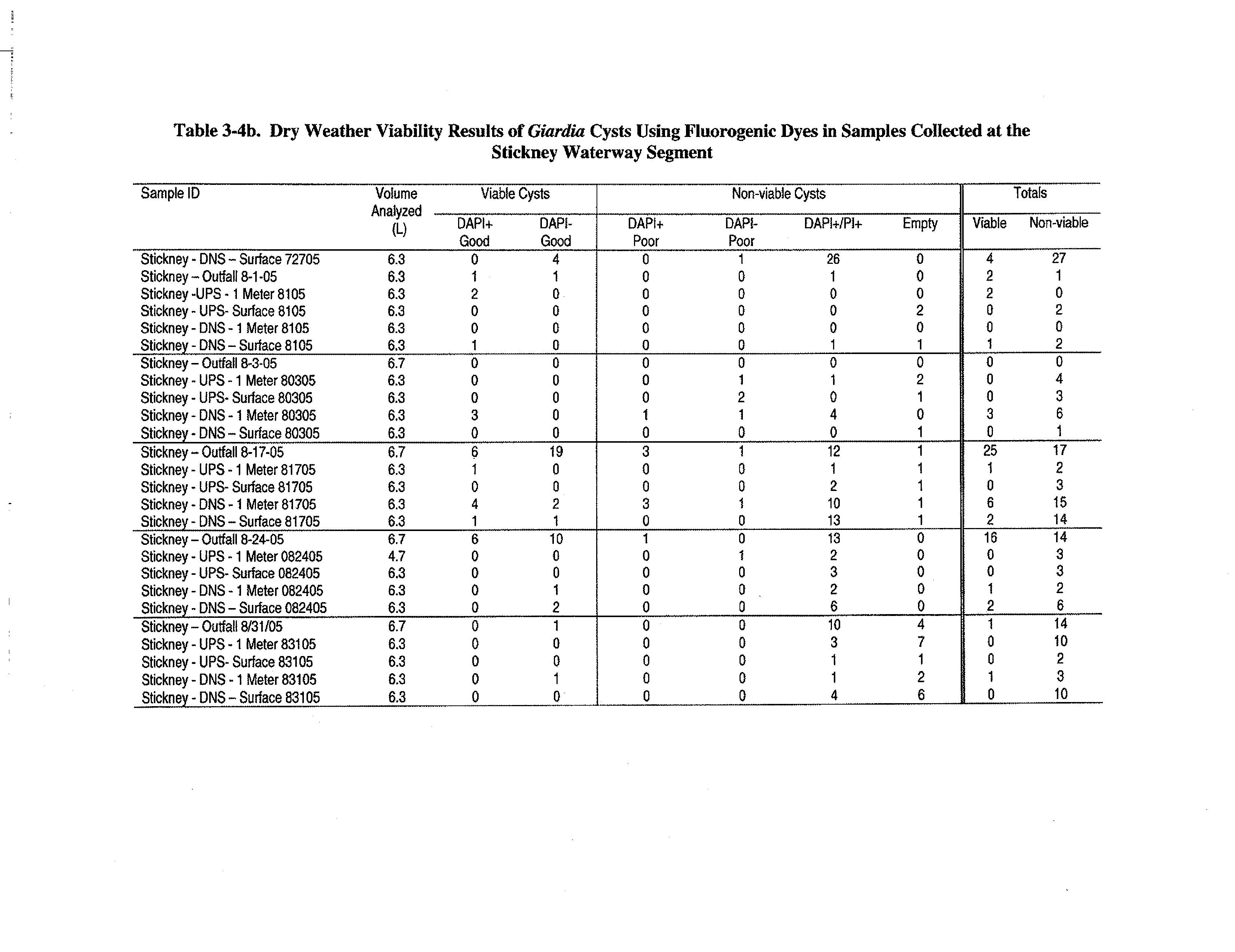
Table 3-4b:
Dry Weather Viability Results of
Giardia
Cysts Using Fluorogenic Dyes
in Samples Collected at the Stickney Waterway Segment
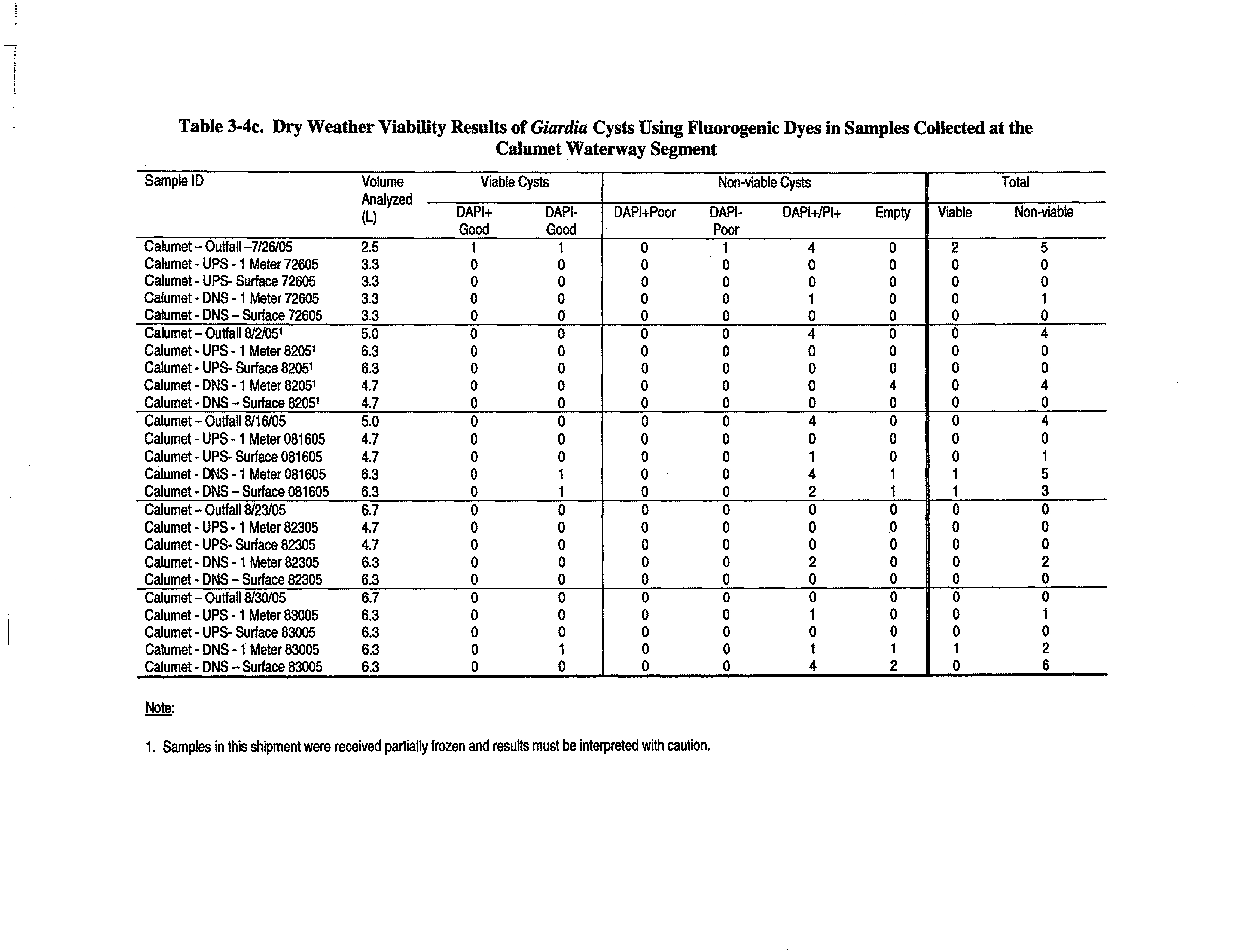
Table 3-4c:
Dry Weather Viability Results of
Giardia
Cysts Using Fluorogenic Dyes
in Samples Collected at the Calumet Waterway Segment
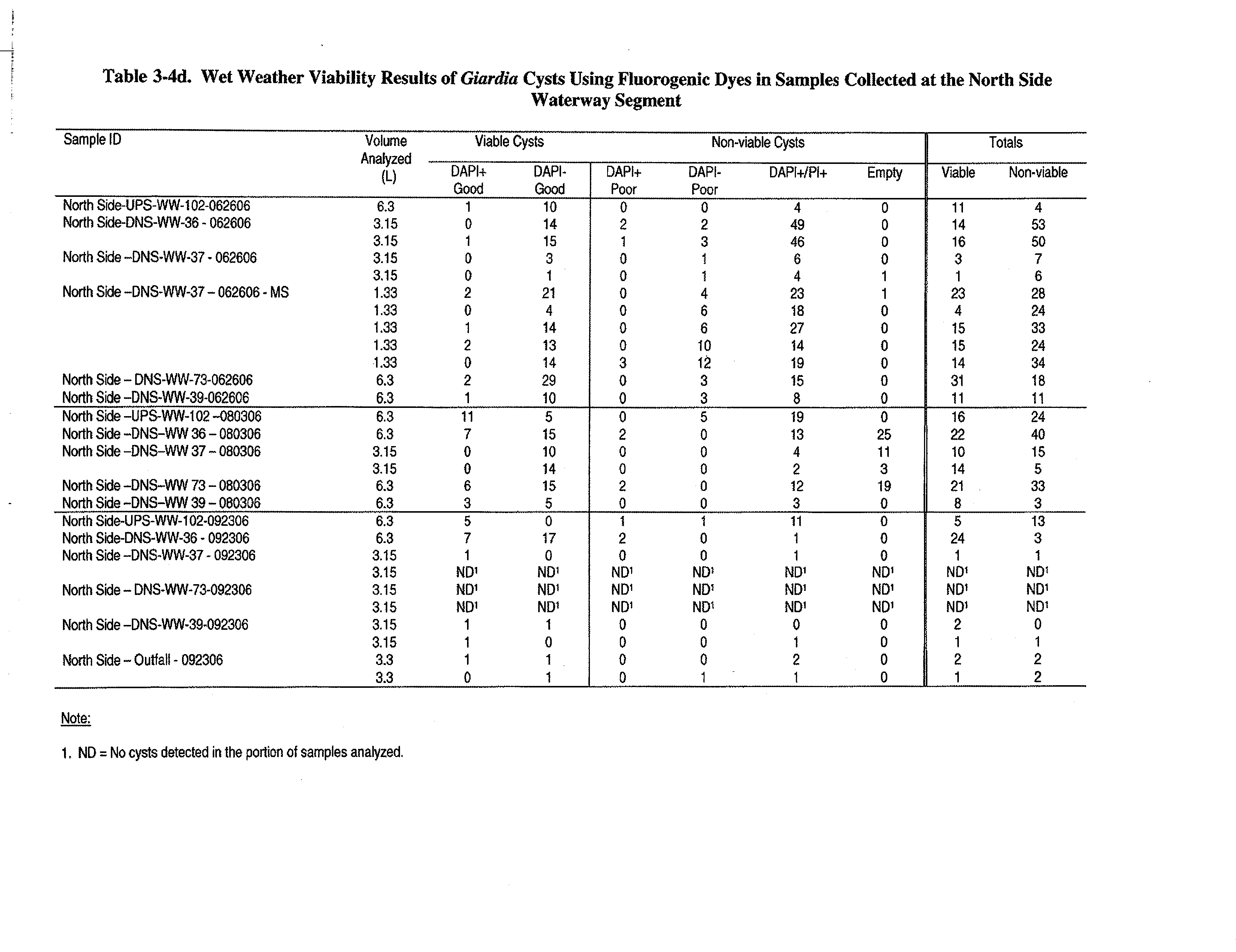
Table 3-4d:
Wet Weather Viability Results of
Giardia
Cysts Using Fluorogenic Dyes
in Samples Collected at the North Side Waterway Segment
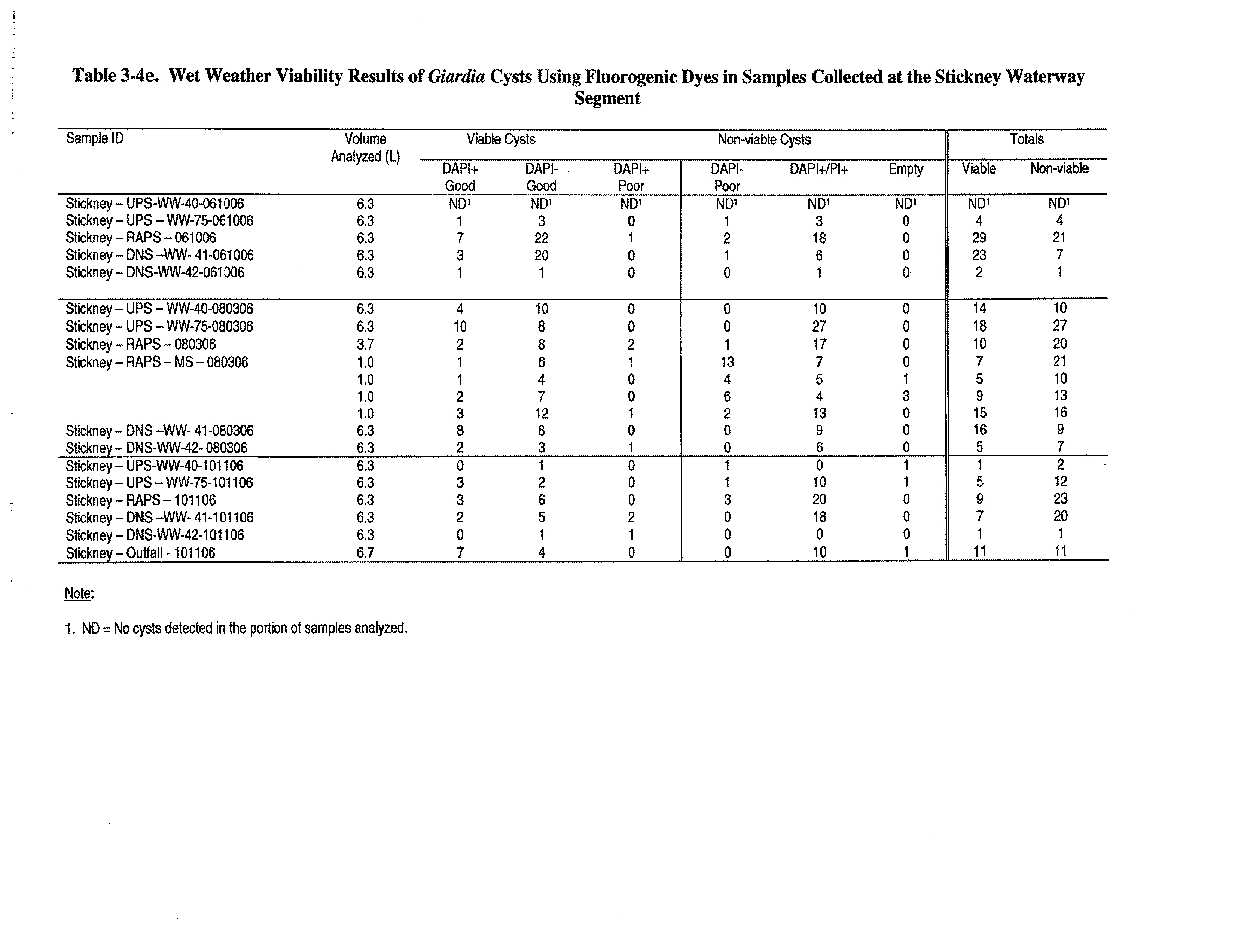
Table 3-4e:
Wet Weather Viability Results of
Giardia
Cysts Using Fluorogenic Dyes
in Samples Collected at the Stickney Waterway Segment
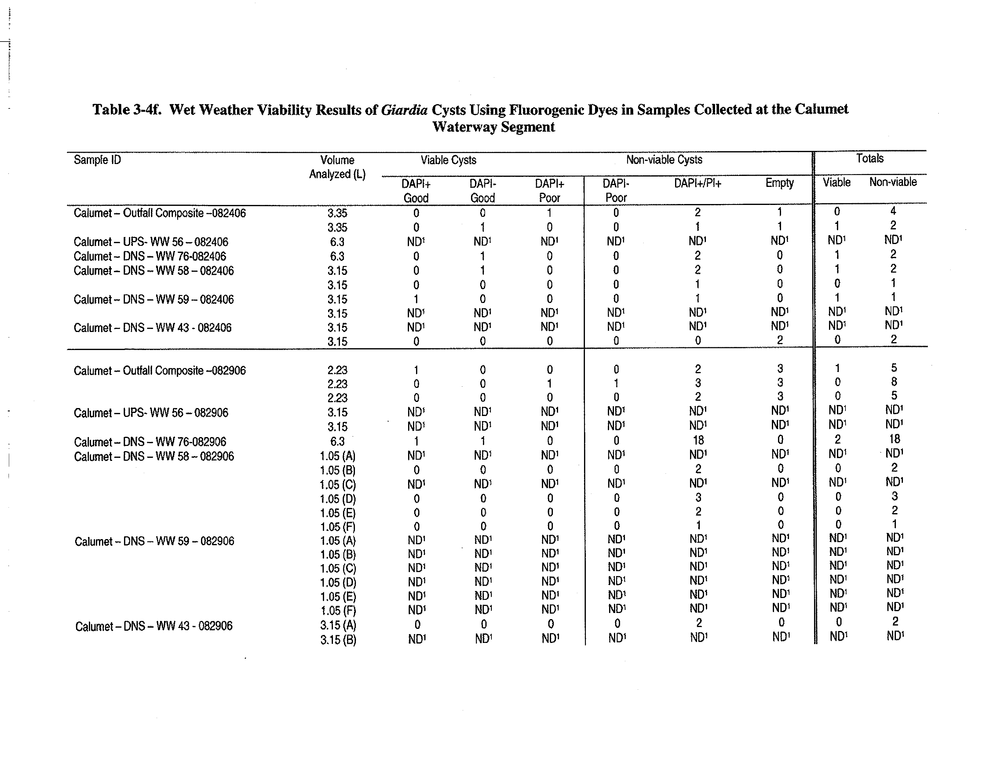
Table 3-4f:
Wet Weather Viability Results of
Giardia
Cysts Using Fluorogenic Dyes
in Samples Collected at the Calumet Waterway Segment
Table 3-5a:
Summary of the North Side Dry Weather Enteric Virus Results
Table 3-5b:
Summary of the Stickney Dry Weather Enteric Virus Results
Table 3-5c:
Summary of the Calumet Dry Weather Enteric Virus Results
Table 3-5d:
Summary of the North Side Wet Weather Enteric Virus Results
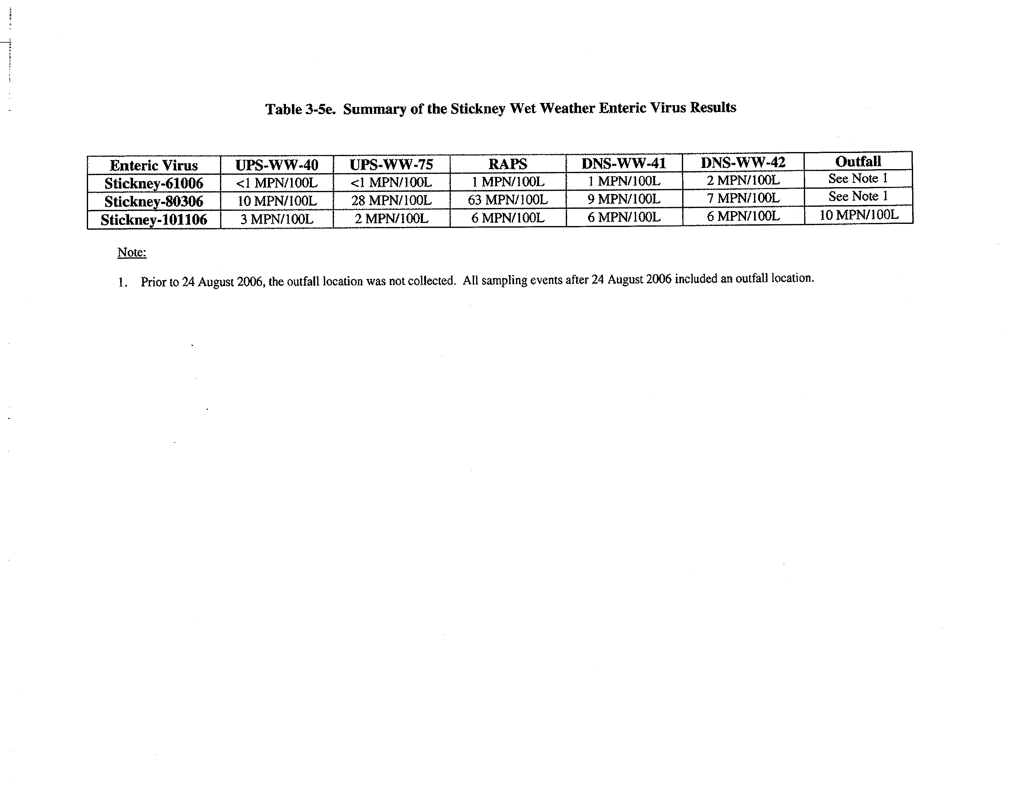
Table 3-5e:
Summary of the Stickney Wet Weather Enteric Virus Results
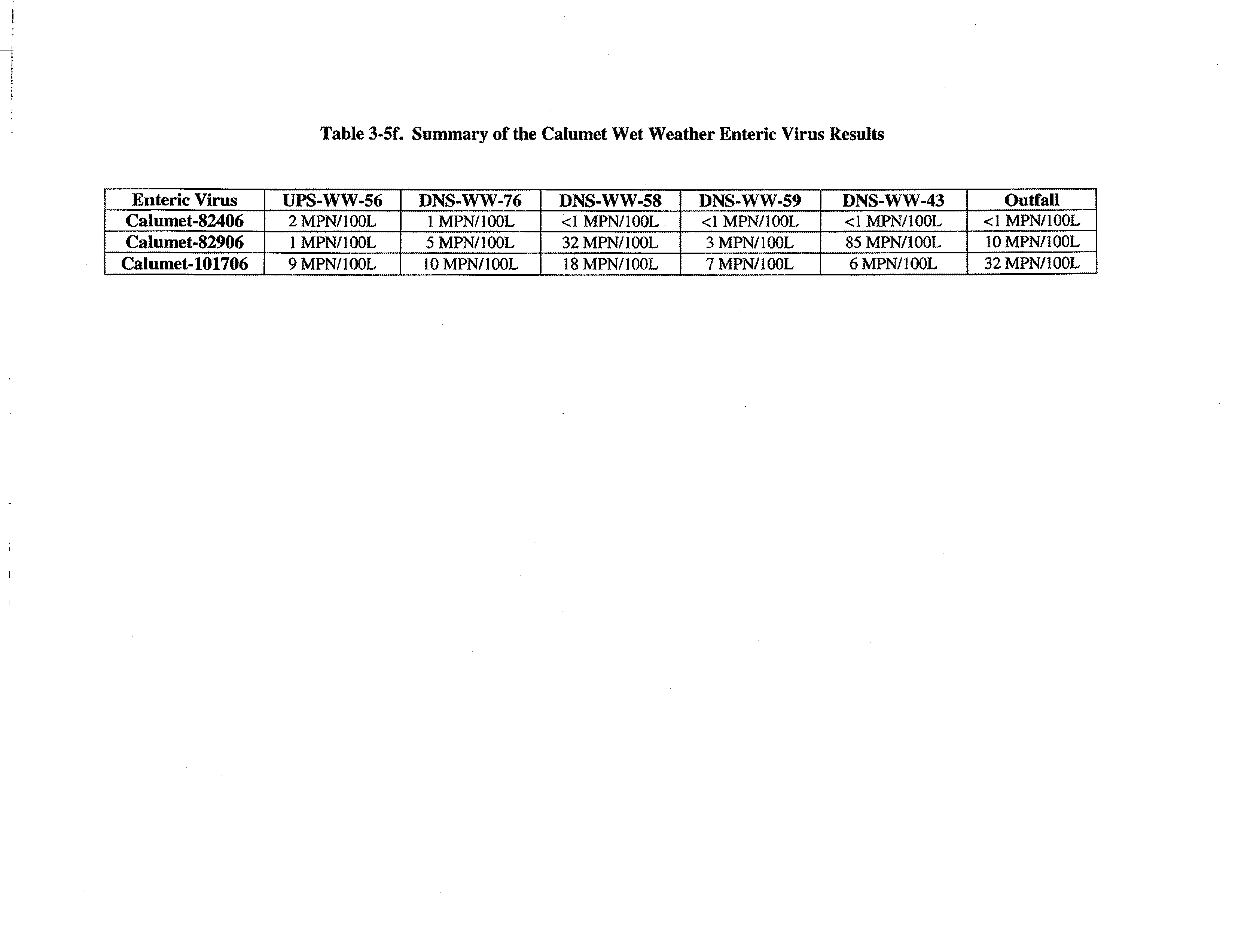
Table 3-5f:
Summary of the Calumet Wet Weather Enteric Virus Results
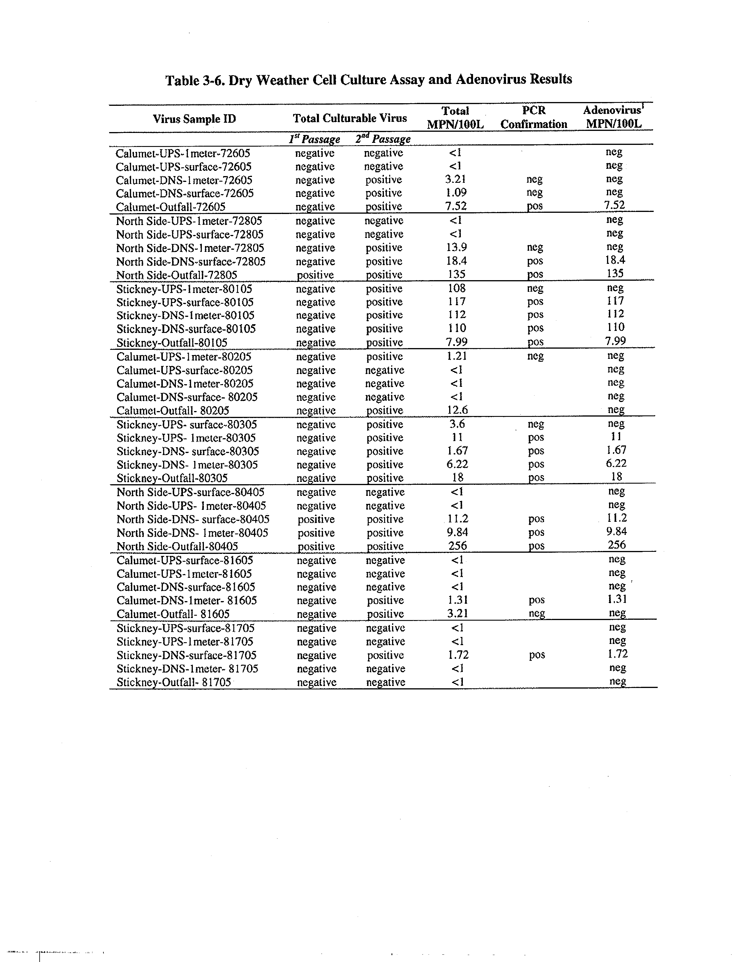
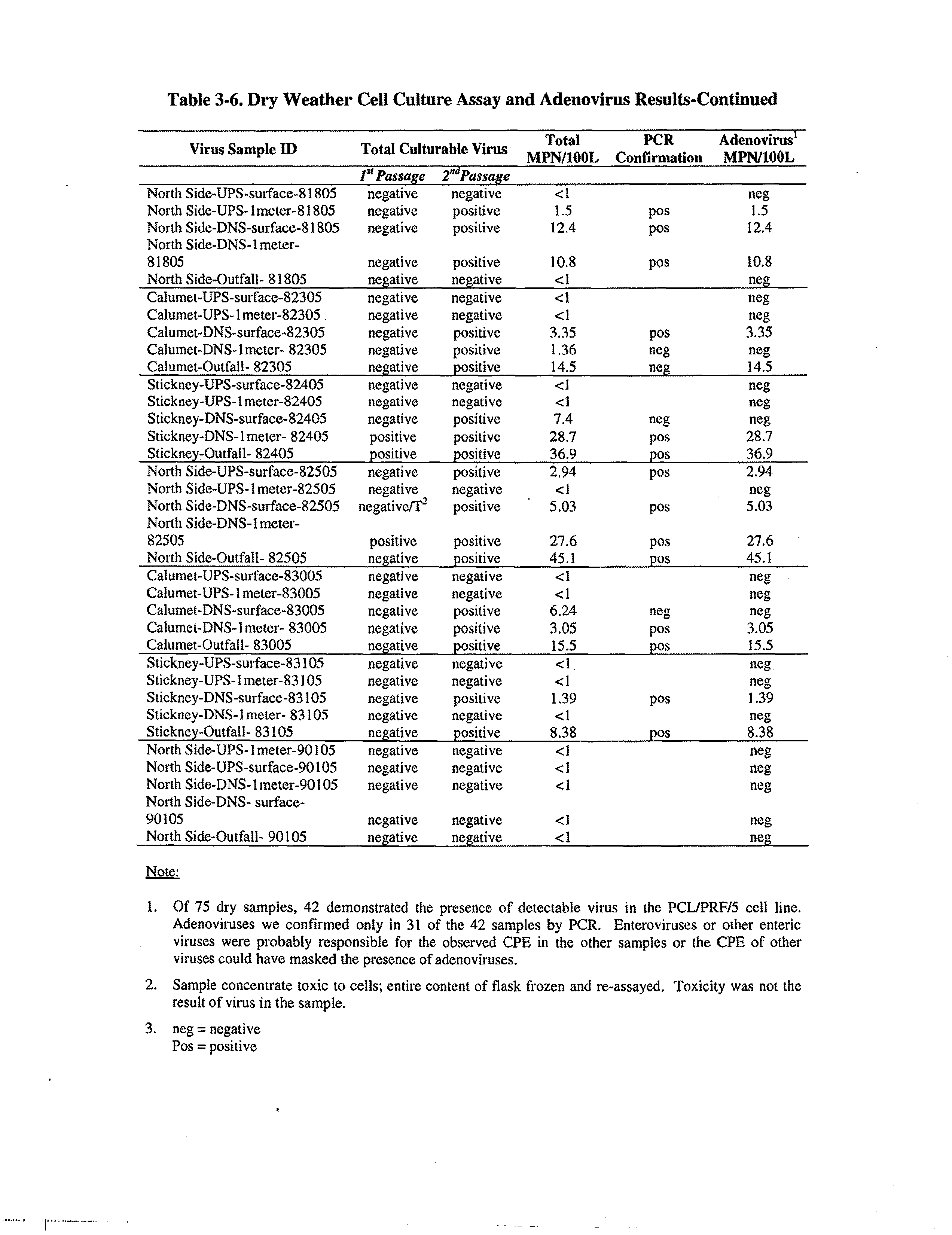
Table 3-6:
Dry Weather Cell Culture Assay and Adenovirus Results
Table 3-7:
Dry Weather Norovirus
(Calicivirus)
Results
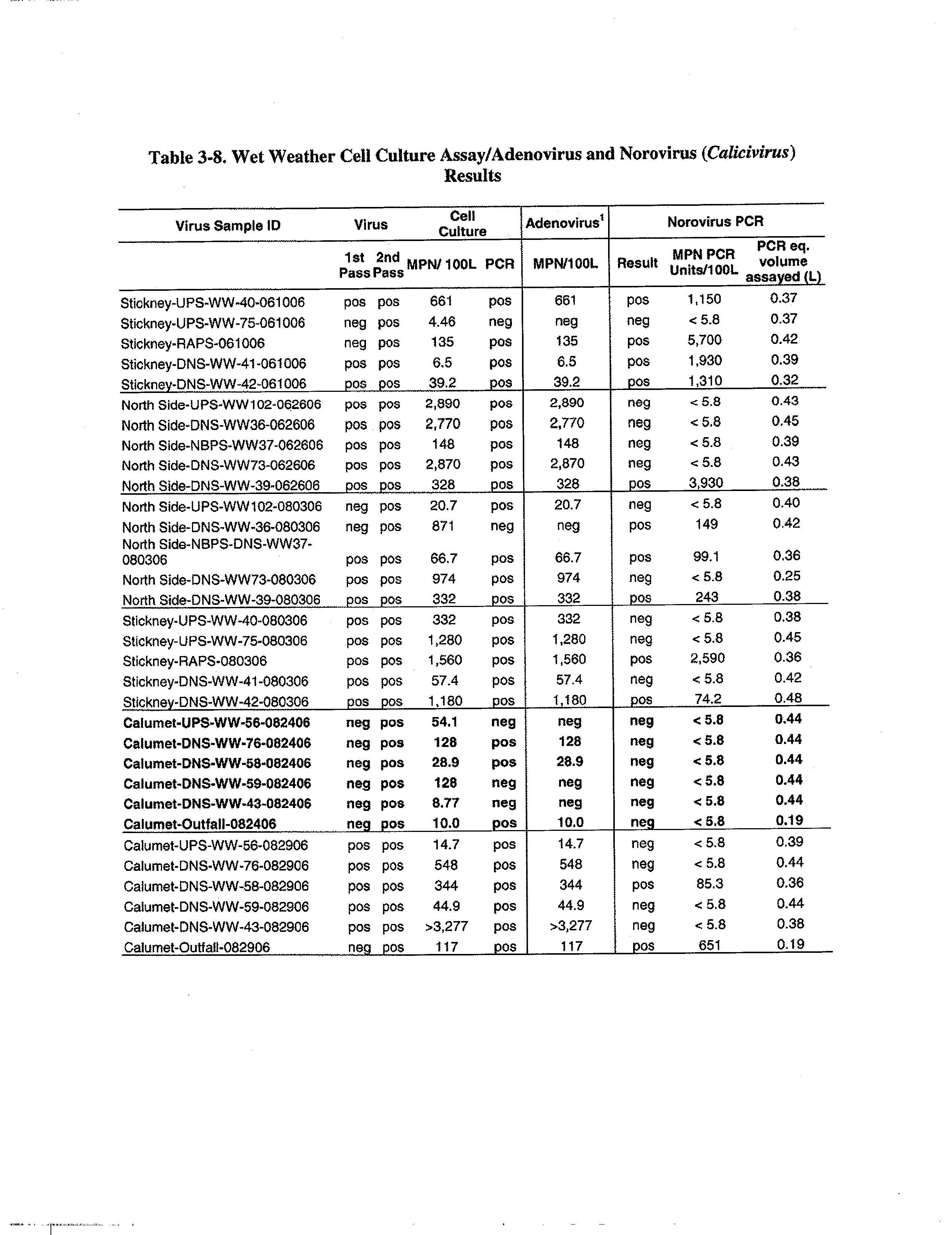
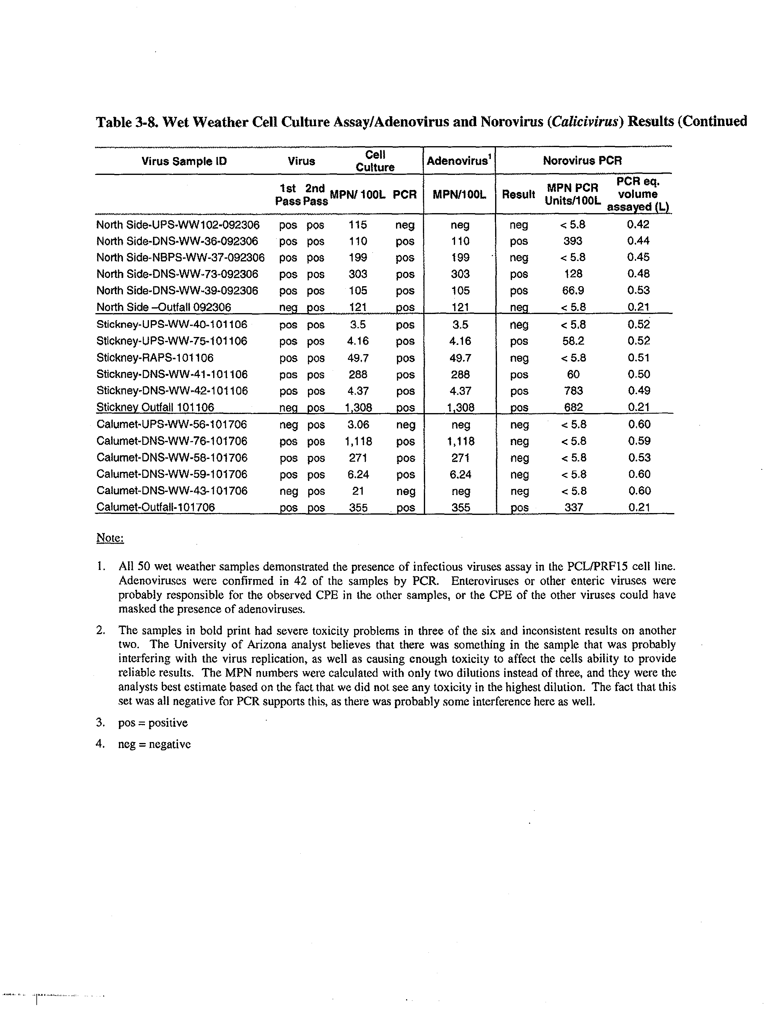
Table 3-8:
Wet Weather Cell Culture Assay/Adenovirus Results and Norovirus
(Calicivirus)
Results
Table 3-9:
Summary of Dry Weather Virus Detections (%) and Detectable
Concentration Ranges
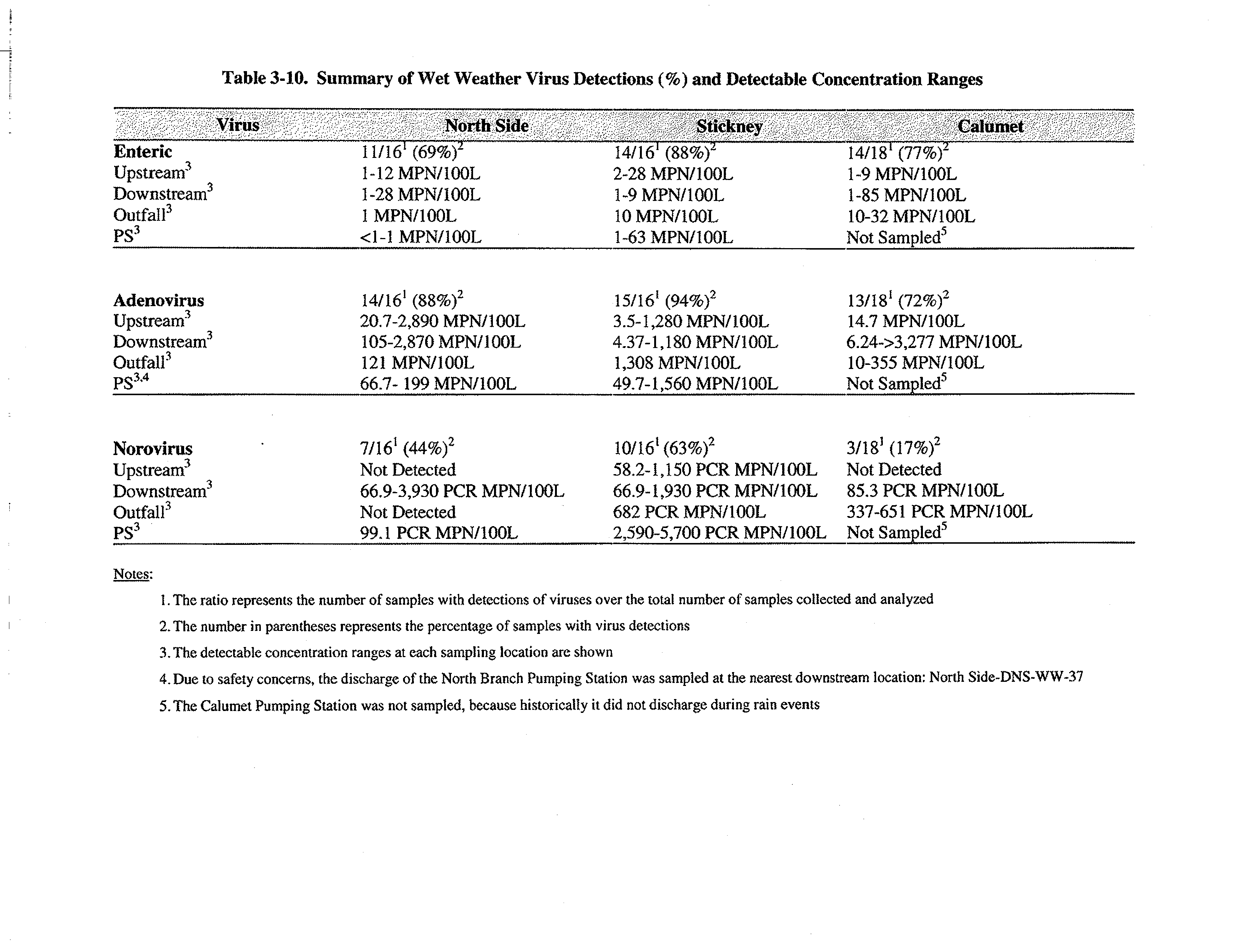
Table 3-10:
Summary of Wet Weather Virus Detections (%) and Detectable
Concentration Ranges
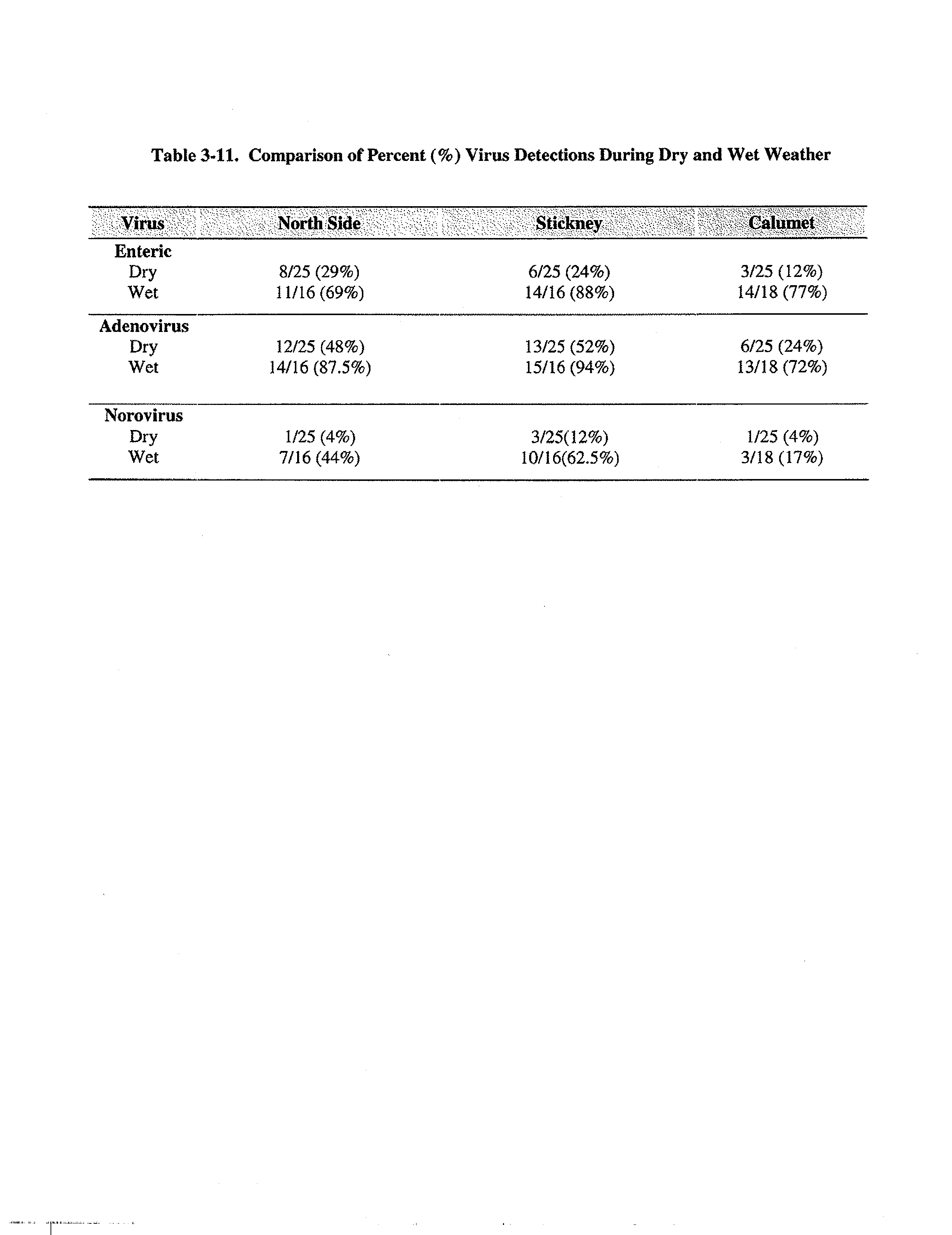
Table 3-11:
Comparison of Percent (%) Virus Detections During Dry and Wet
Weather
Table 4-1:
Summary of Disinfectant Characteristics
Table 4-2:
List of DBPs and Disinfection Residuals
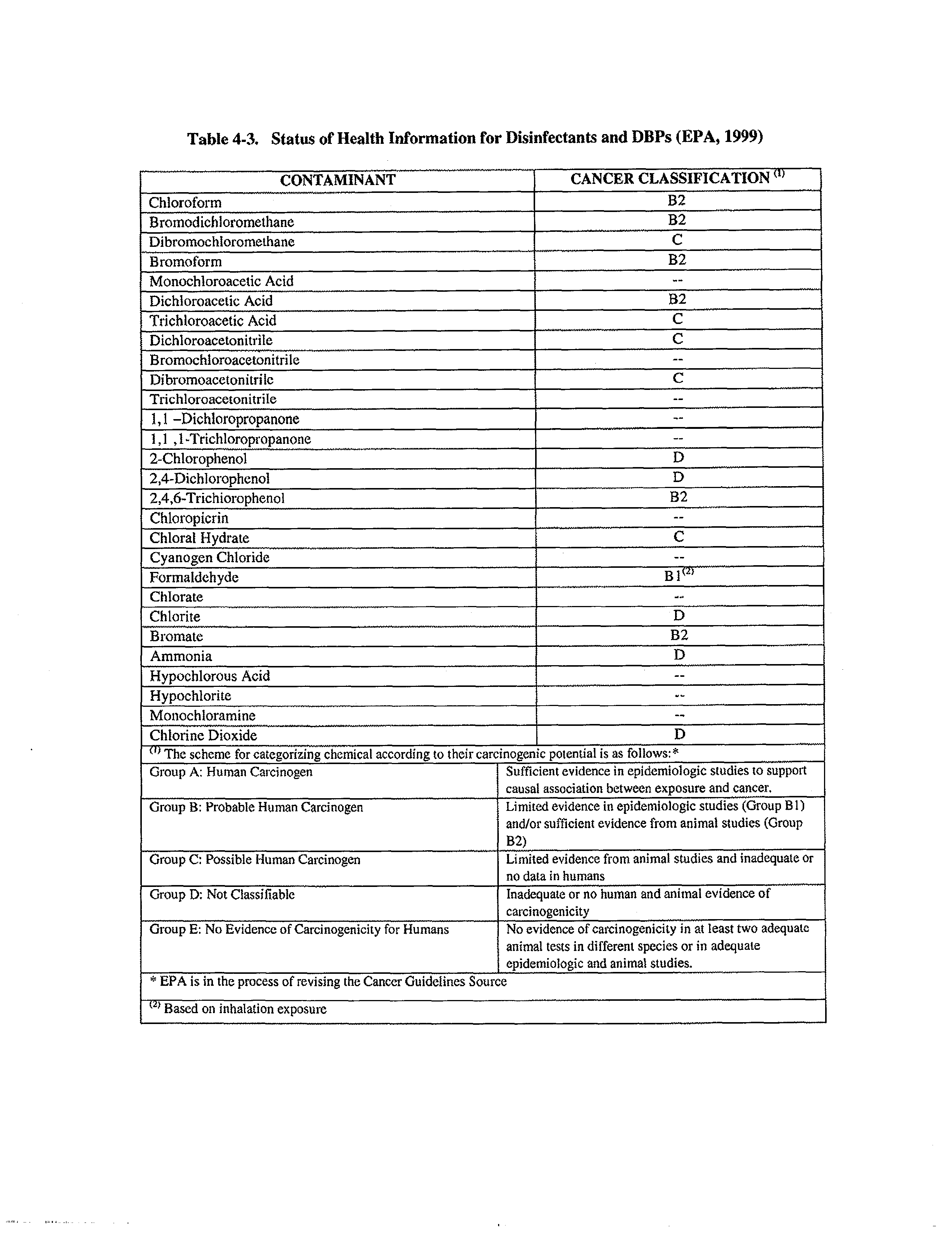
Table 4-3:
Status of Health Information for Disinfectants and DBPs
Table 4-4:
Principal Known By-products of Ozonation
Table 4-5:
Ozone Disinfection Studies Involving Indicator Bacteria
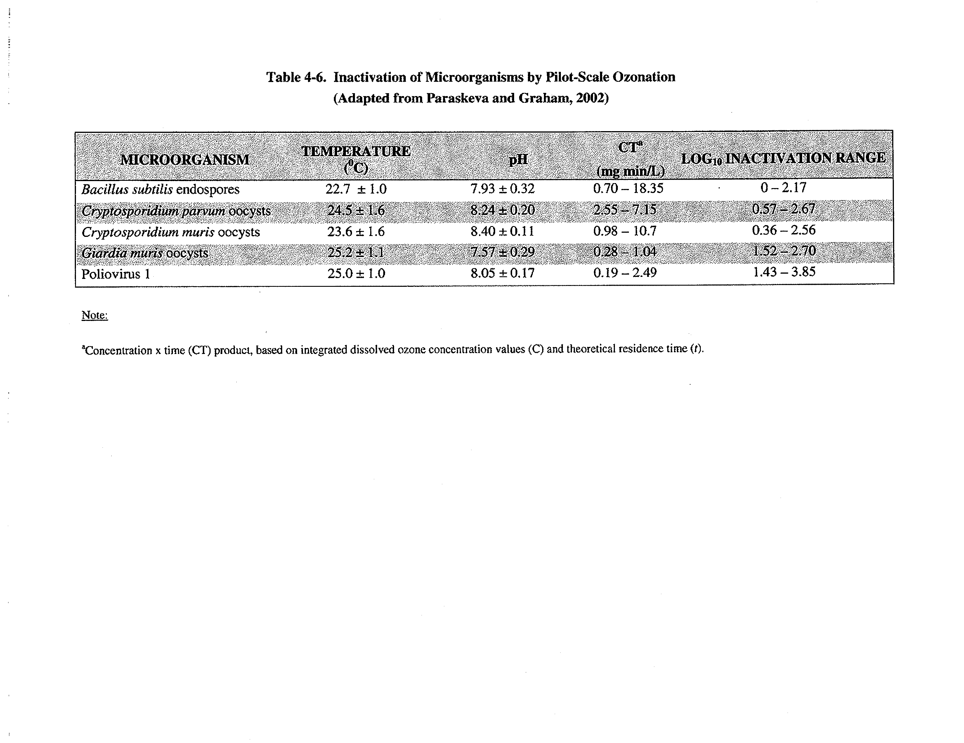
Table 4-6:
Inactivation of Microorganisms by Pilot-Scale Ozonation
Final
Wetdry-April 2008
V
LIST OF TABLES (
Continued)
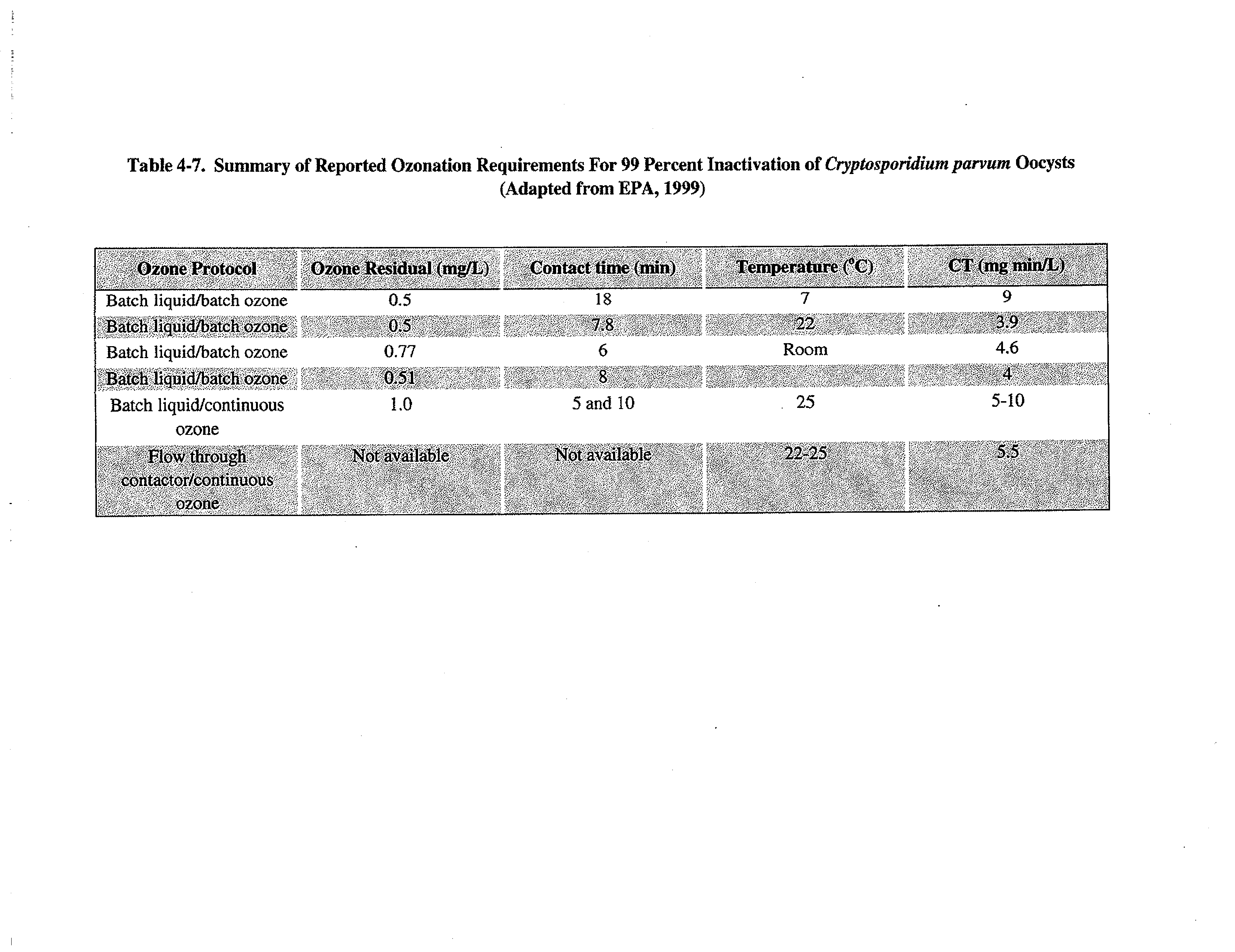
Table 4-7:
Summary of Reported Ozonation Requirements for 99% (2-Lag)
Inactivation of
Cryptosporidiwn parvum
Oocysts
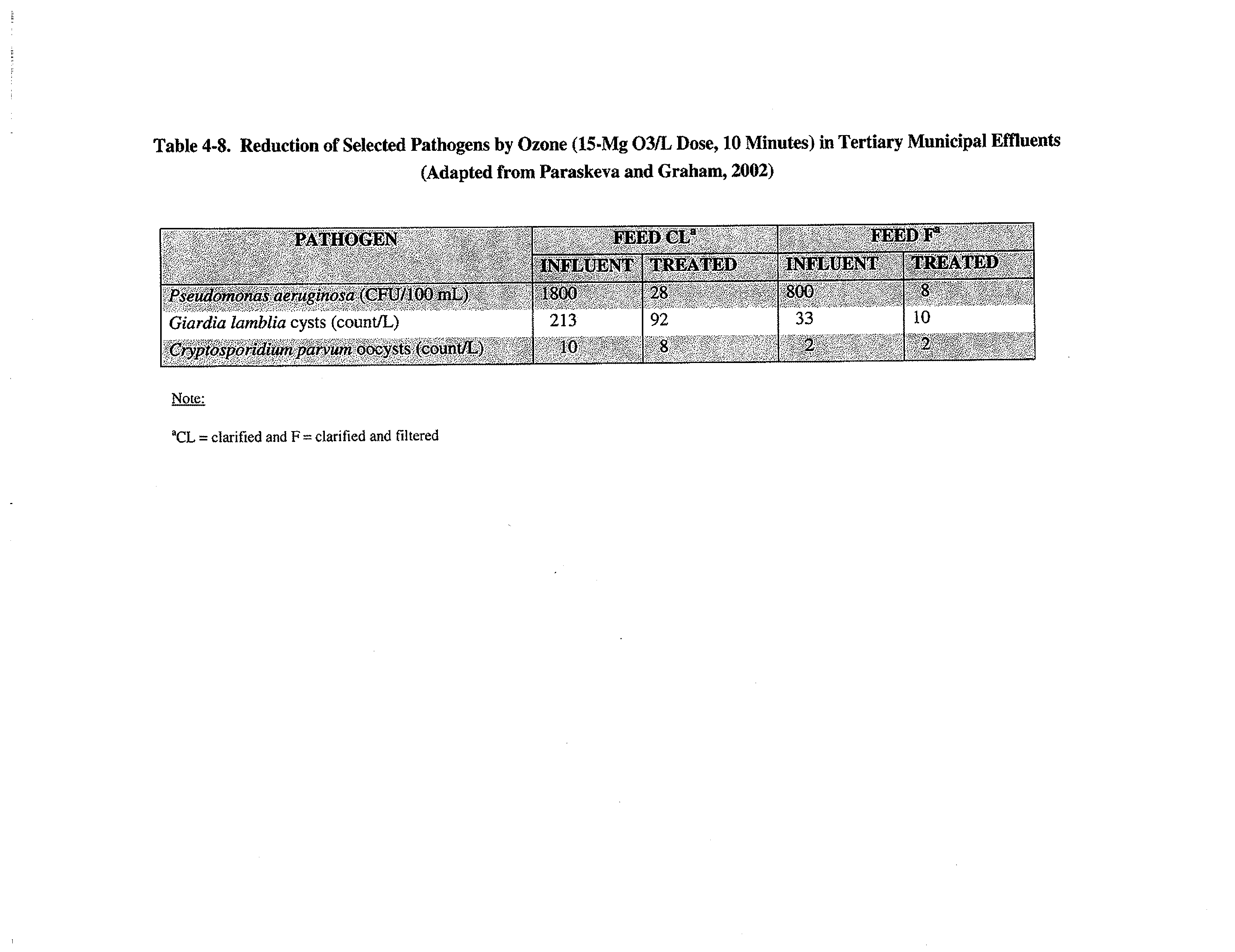
Table 4-8:
Reduction of Selected Pathogens by Ozone in Tertiary Municipal
Effluents
Table 4-9:
Summary of CT Values for 99% Inactivation of Selected Viruses by
Various Disinfectants at 5°C
Table 4-10:
LOG,a Reductions Achieved for Coliphage During Disinfection of
Secondary Effluent by UV Irradiation and Chlorination
Table 4-11:
Summary of Pathogen Disinfection Efficiencies
Table 5-1:
UAA General Activity Groups and Risk Assessment Categories
Table 5-2:
Proportion of Users in Each Risk Assessment Activity Category by
Waterway
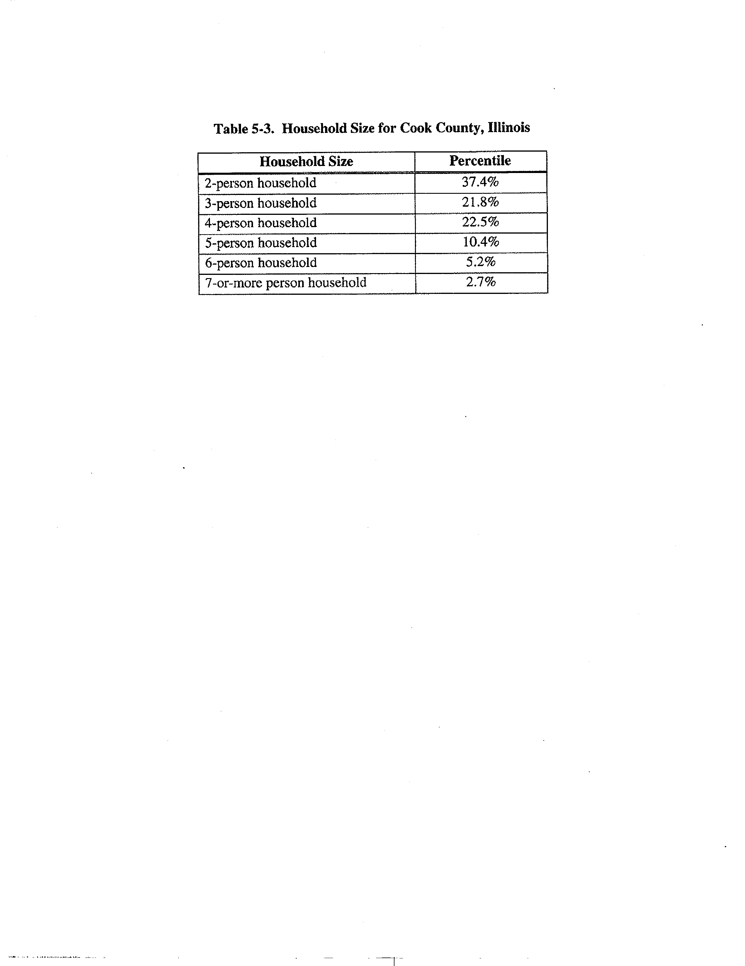
Table 5-3:
Household Size for Cook County, Illinois
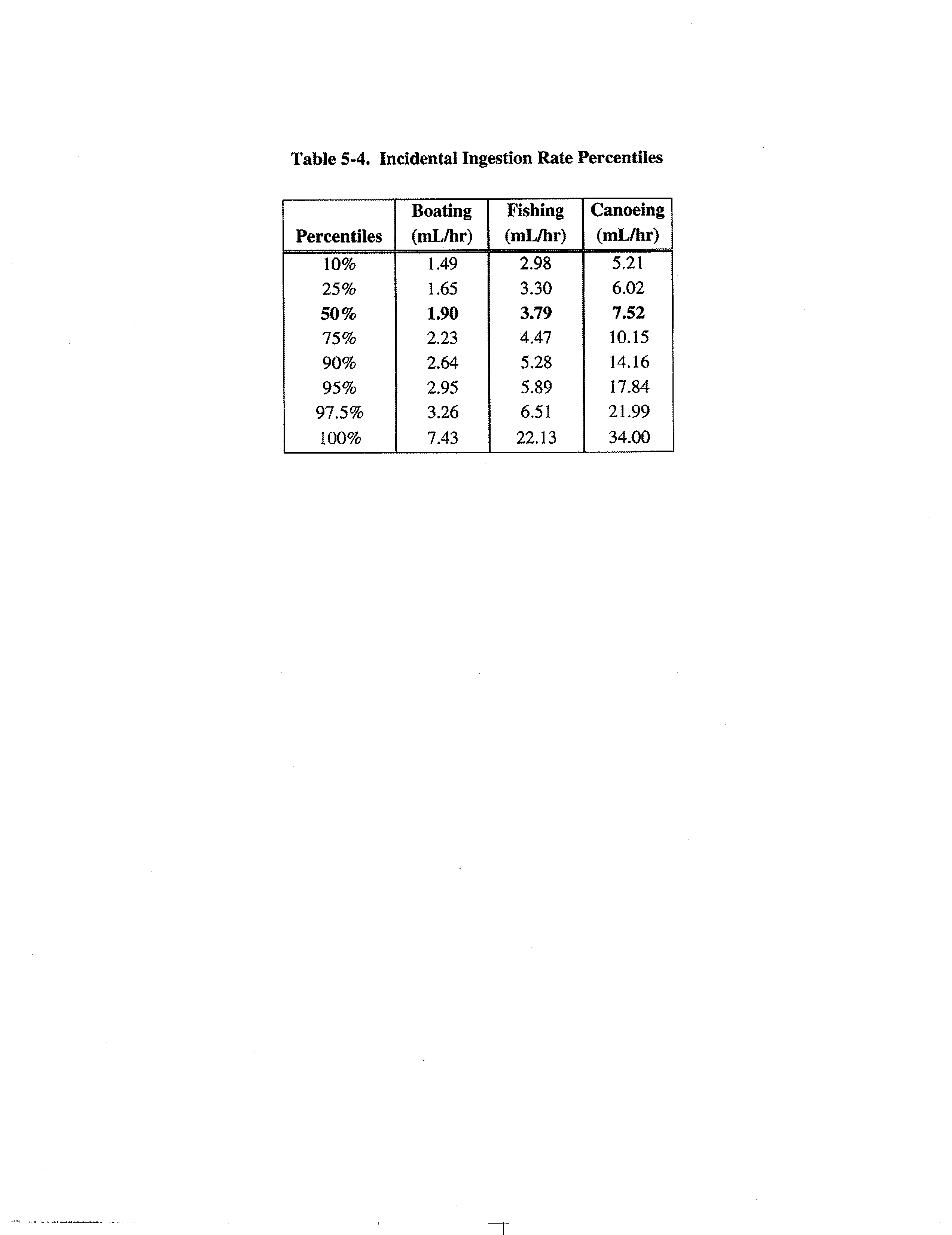
Table 5-4:
Incidental Ingestion Rate Percentiles
Table 5-5:
Summary of Dose-Response Parameters Used for Risk Assessment
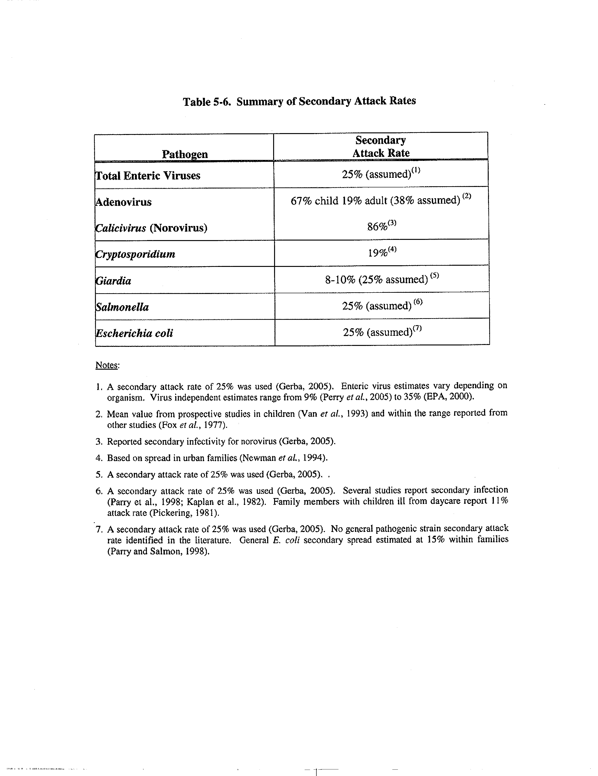
Table 5-6:
Summary of Secondary Attack Rates
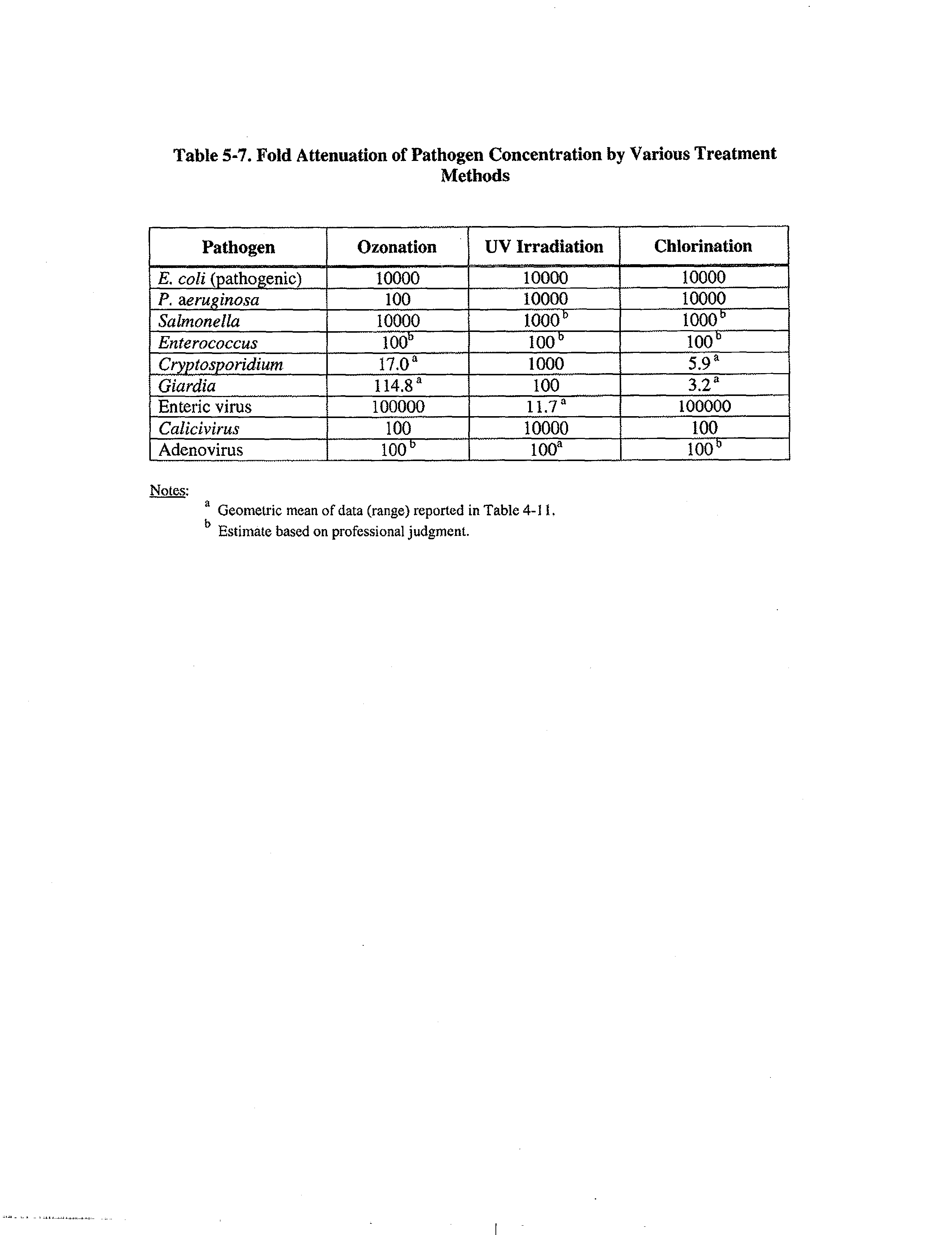
Table 5-7:
Fold Attenuation of Pathogen Concentration by Various Treatment
Methods
Table 5-8:
Proportion of Weather Days in Recreational Year
Table 5-9:
Total Expected Illnesses per 1,000 Exposures Using Different Estimates of
Pathogen Concentrations with No Effluent Disinfection
Table 5-10:
Criteria for Indicators for Bacteriological Densities
Table 5-11:
Proportion of Recreational User Type Contributing to Gastrointestinal
Expected Illnesses with No Effluent Disinfection
Table 5-12
Stratified
Risk Estimates - Estimated Illness Rates Assuming Single
Recreational Use with No Effluent Disinfection
Table 5-13:
Breakdown of Illnesses per 1,000 Exposures for Combined Wet and Dry
Weather Samples with No Effluent Disinfection
Table 5-14:
Total Expected Primary Illnesses per 1,000 Exposures Under Combined
Dry and Wet Weather Using Different Disinfection Techniques
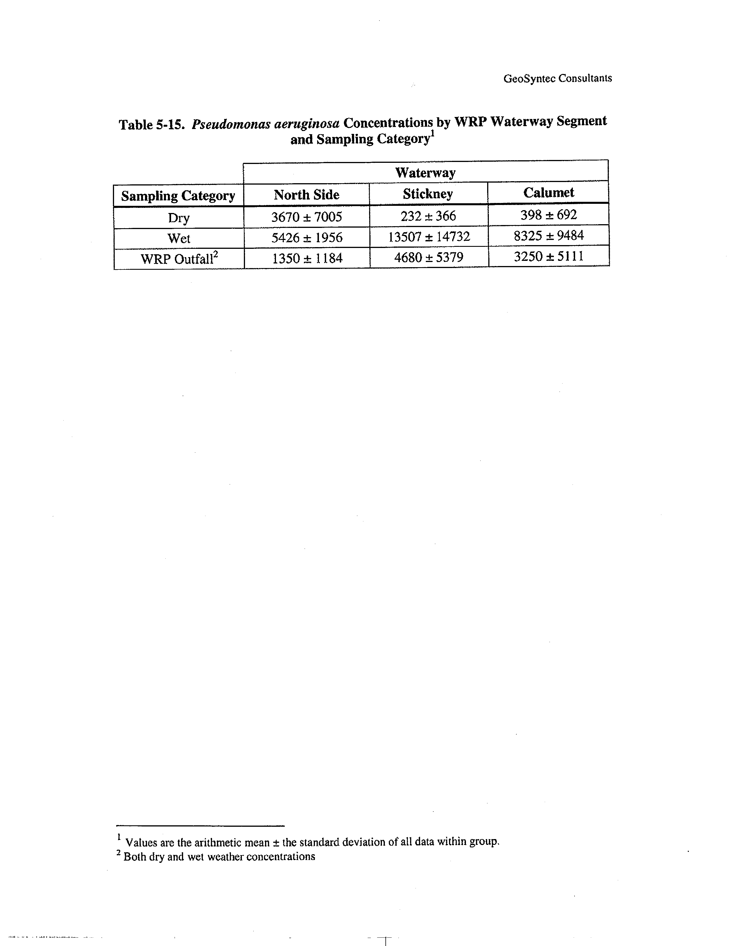
Table 5-15:
Pseudomonas aeruginosa
Concentrations by
WRP Waterway Segment
and Sampling Category
Table 5-16:
Sensitivity Analysis for Risks of Illness in WRP Segments
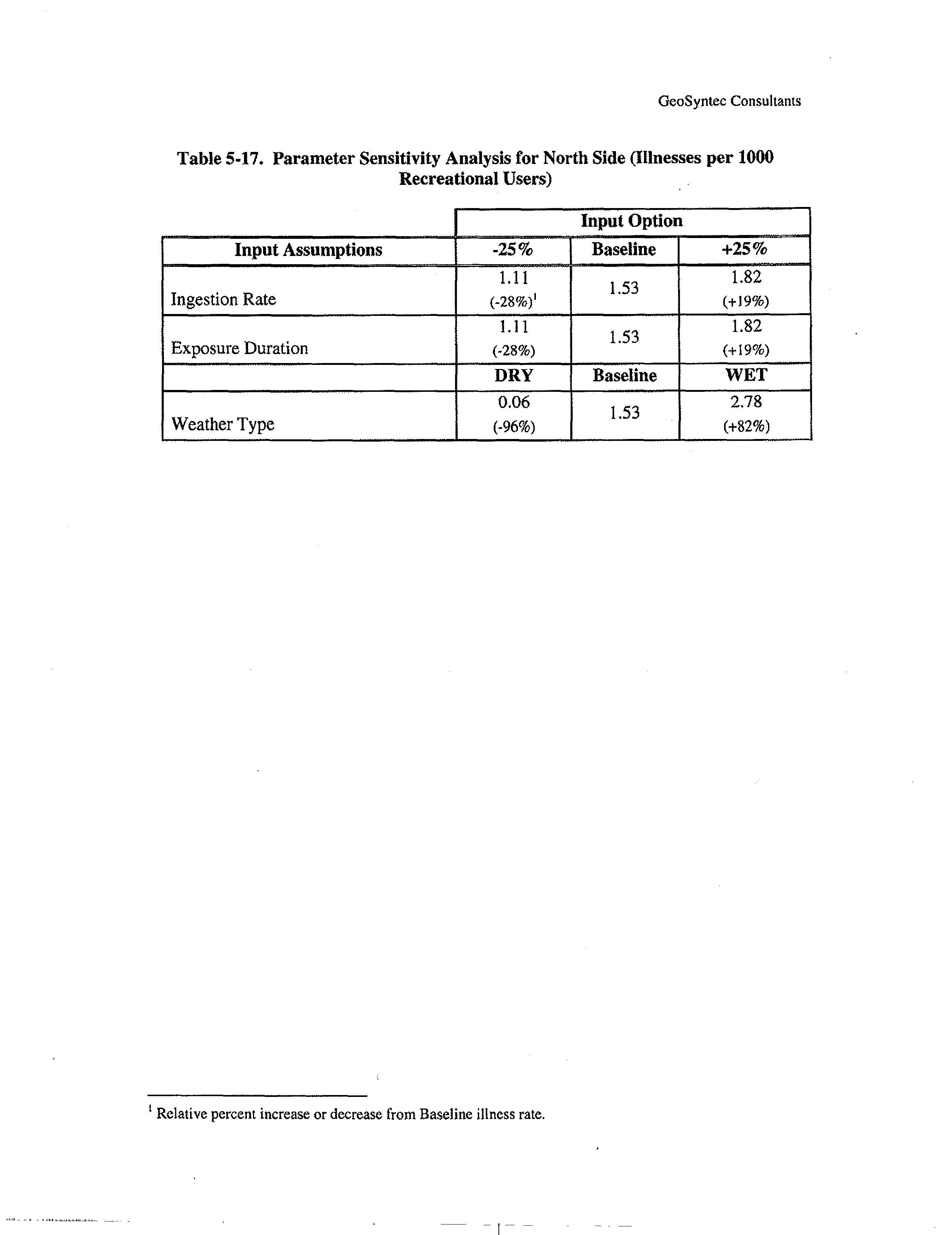
Table 5-17:
Parameter Sensitivity Analysis for North Side (Illnesses per 1,000
Recreational Users)
Final Wetdry-Apil 2008
vi
Geosynte&
consultants
LIST OF FIGURES
Figure ES-1:
Figure ES-2:
Figure 1-1:
Figure 2-1:
Figure 2-2:
Figure 2-3:
Figure 3-1:
Figure 3-2:
Figure 3-3:
Figure 3-4:
Figure 3-5:
Figure 3-6:
Figure 3-7:
Figure 3-8:
Figure 3-9:
Figure 3-10:
Figure 3-11:
Figure 3-12:
Figure 3-13:
Figure 3-14:
Figure 3-15:
Figure 3-16:
Figure 3-17:
Figure 3-18:
Figure 3-19:
Chicago Waterway System - Dry Weather Sampling Locations
Chicago Waterway System - Wet Weather Sampling Locations
Chicago Waterway System
Chicago Waterway System Dry Weather Sampling Locations
Chicago Waterway System Wet Weather Sampling Locations
Typical Filter Apparatus
North Side Dry Weather Bacteria Histograms
Stickney Dry Weather Bacteria Histograms
Calumet Dry Weather Bacteria Histograms
ANOVA
Results: Dry Weather E.
coli
- vs
.
Site
,
Location, Depth
ANOVA
Results: Dry Weather Fecal Conform
-
vs. Site, Location, Depth
ANOVA Results:
Dry Weather
Enterococcus
-
vs. Site, Location, Depth
ANOVA
Results: Wet Weather
E.
coli
- vs.
Site, Location
ANOVA
Results
:
Wet Weather Fecal Coliform
-
vs. Site, Location
ANOVA
Results:
Wet Weather
Enterococcus
-
vs. Site
,
Location
ANOVA
Results
:
Wet Weather
Pseudomonas aeruginosa-
vs.
Site,
Location
ANOVA Results
: Wet Weather
Salmonella-
vs. Site
,
Location
ANOVA
Results
:
Dry and Wet Weather E.
coli
-
vs.
Site,
Location,
Weather
ANOVA
Results
:
Dry and Wet Weather Fecal Coliform - vs. Site,
Location, Weather
ANOVA
Results
:
Dry and Wet Weather
Enterococcus
-
vs. Site, Location,
Weather
ANOVA Results
: Dry and Wet Weather
Pseudonnonas aeruginosa-
vs.
Site, Location
,
Weather
Geometric Mean Dry Weather Bacteria Concentrations at North Side
Geometric Mean Dry Weather Bacteria Concentrations at Stickney
Geometric Mean Dry Weather Bacteria Concentrations at Calumet
Wet Weather Geometric Mean Bacteria Concentrations by Location (UPS,
DNS, OUTFALL)
at North Side
,
Stickney and Calumet
(
cfu/100mL;
Salmonella
in MPN/L)
Final Wetdry-April 2008
Vii
LIST OF FIGURES
(Continued)
Figure 3-20:
Dry and Wet Weather Geometric Mean Bacteria Concentrations by WRP
(including OUTFALLS, UPS, DNS) (cfu/100mL;
Salmonella
in
MPN/L)
Figure 3-21:
North Side Dry Weather Spatial Box Plots of Bacteria Concentrations
Figure 3-22:
Stickney Dry Weather Spatial Box Plots of Bacteria Concentrations
Figure 3-23:
Calumet Dry Weather Spatial Box Plots of Bacteria Concentration
Figure 3-24:
North Side Wet Weather Temporal Percentile Box Plots of Bacteria
Concentrations
Figure 3-25:
Stickney Wet
Weather Temporal Percentile Box Plots of Bacteria
Concentrations
Figure 3-26:
Calumet Wet
Weather Temporal Percentile Box Plots of Bacteria
Concentrations
Figure 4-1:
Conceptual Representation of the Possible Fates of Bacteria Disinfectant
Exposure
Figure 5-1:
CWS Microbial Risk Assessment Segments
Figure 5-2:
Incidental Ingestion Rate Distribution for Canoeists (mUhr)
Figure 5-3:
Duration Distribution for Canoeists
Figure 5-4:
Estimated Pathogen Concentration between Wet and Dry Sampling Events
Final WCUiry-Apri12008
Viii
Geosyntec°
consultants
LIST OF ATTACHMENTS
Attachment A: Bacteria Correlations
Final Wetdry-April 2008
ix
Geosynte&
consultants
LIST OF APPENDICES
Appendix A-1: MWRDGC Dry Weather Field Sampling Forms
Appendix A-2: MWRDGC Wet Weather Field Sampling Forms
Appendix B-1: Dry Weather HML Analytical Results
Appendix B-2:
Wet Weather HML Analytical Results
Appendix C-1: Dry Weather CEC Analytical Report
Appendix C-2: Wet Weather CEC Analytical Report
Appendix D-1: Dry Weather University of Arizona Analytical Results
Appendix D-2: Wet Weather University of Arizona Analytical Results
Final Wetdry-April 2008
x
Geosynte&
consultants
LIST OF ACRONYMS
ANOVA
Analysis of Variance
AWQM
Ambient Water Quality Monitoring
BEACH
Beaches Environmental Assessment and Coastal Health
BGMK
Blue Green Monkey Kidney
BR
Backflow Regulator
CCL
Contaminant Candidate List
CDC
Center for Disease Control
CEC
Clancy Environmental Consultants, Inc.
COD
Chemical Oxygen Demand
CLHA
Cecil Lue-Ring and Associates
CPE
Cytopathic Effects
CSC
Calumet-Sag Channel
CSO
Combined Sewer Overflow
CSSC
Chicago Sanitary and Ship Canal
CT
Contact Time
CDF
Cumulative Distribution Function
CWA
Clean Water Act
CWS
Chicago Area Waterway System
DAPI
4',6-diamidino-2-phenylindole
DBPs
Disinfection Byproducts
DIC
Differential Interference Contrast
DPR
Des Plaines River
DNS
Downstream
DQO
Data Quality Objective
E. soli
Escherichia soli
EPA
US Environmental Protection Agency
FA
Fluorescence Assay
FITC
Fading/Diffusion Of Fluorescent Isothiocyanate
FS
Flowing Stream
Geosyntec
Geosyntec Consultants
GPS
Global Positioning System
HAV
Hepatitis A Virus
HEV
Hepatitis E Virus
HML
Hoosier Microbiological Laboratory, Inc.
IDPH
Illinois Department of Public Health
IEPA
Illinois Environmental Protection Agency
IPCB
Illinois Pollution Control Board
LCR
Little Calumet River
LP&L
Lockport Powerhouse and Lock
MG
Million Gallons
MGD
Million Gallons per Day
MF
Membrane Filtration
MLE
Maximum Likelihood Estimation
Final Wetdry-April 2008
Xi
Geospte&
consultants
LIST OF ACRONYMS (
Continued)
MPN
Most Probable Number
MS
Matrix Spike
MWRDGC
Metropolitan Water Reclamation District of Greater Chicago
NAC
Negative Assay Control
NOM
Natural Organic Matter
NPDES
National Pollutant Discharge Elimination System
NSC
North Shore Channel
NTU
Nephelometric Turbidity Units
OPR
Ongoing Precision And Recovery
PAC
Positive Assay Control
PCR
Polymerase Chain Reaction
PDF
Probability Density Function
PMF
Probability Mass Function
PEC
Patterson Environmental Consultants
PFU
Plaque Forming Units
PR
Regulator Module
QA
Quality Assurance
QC
Quality Control
QAPP
Quality Assurance Project Plan
QMRA
Quantitative Microbial Risk Assessment
RFP
Request for Proposal
RT
Reverse Transcriptase
SAC
Senior Advisory Committee
SAP
Sampling and Analysis Plan
SC
Specific Conductance
SF
Swivel Female Insert
SOP
Standard Operating Procedure
SWW
Significant Wet Weather
UAA
Use Attainability Analysis
UV
Ultraviolet
UPS
Upstream
VIRADEL
Virus Adsorption-Elution
WCC
Waterway Control Center
WHO
World Health Organization
WRP
Water Reclamation Plant
Final Wetdry-April 2008'
Xii
Geosyntec°
consultants
EXECUTIVE SUMMARY
The Metropolitan
Water Reclamation District of Greater Chicago (MWRDGC or
District) has retained The Geosyntec Team, which includes Geosyntec Consultants
(Geosyntec) and its subcontractors, Patterson Environmental Consultants (PEC); Cecil
Lue-Hing & Associates (CLHA); Dr. Charles Gerba of the University of Arizona (UA);
Hoosier
Microbiological
Laboratory,
Inc.
(HML); and Clancy Environmental
Consultants, Inc. (CEC) to perform a Risk Assessment of Human Health Impacts of
Disinfection Vs. No Disinfection of the Chicago Area Waterways System (CWS).
The CWS consists of 78 miles of canals, which serve the Chicago area for two principal
purposes: (1) the drainage of urban storm water runoff and treated municipal wastewater
effluents from the District's three major water reclamation plants (WRP) (North Side,
Stickney and Calumet), and (2) the support of commercial navigation (See Figure ES-1).
Approximately 75 percent of the length of the CWS includes manmade canals where no
waterway existed previously, and the remainder includes natural streams that have been
deepened, straightened and/or widened to such an extent that reversion to the natural state
is not possible.
About 70 percent of the annual flows in the CWS are from the discharge
of treated municipal wastewater effluent from the District's WRPs (MWRDGC, 2004).
Over time, there have been major improvements in water quality, altered land use and
additional public access along the CWS.
Such improvements and conditions have
produced both greater opportunity and heightened public interest in environmental and
recreational uses within and along the waterways. Currently, the waterways are used for
recreational boating, canoeing, fishing and other streamside recreational activities. These
waterways also provide aquatic habitat for wildlife.
The Illinois Environmental Protection Agency (IEPA) has conducted a Use Attainability
Analysis (UAA) of the CWS in accordance with 40 CFR 131.10(d). The IEPA and UAA
stakeholders have agreed that swimming and other primary contact recreation should not
be considered as a viable designated use of the CWS. The IEPA initially attempted to
develop water quality standards for the CWS based on the
Ambient Water Quality
Criteria for Bacteria-1986
(EPA, 1986) and EPA guidance (EPA, 2003). In order to
Final Wetdry-April 2008'
xiii
Geosyntec
consultants
assist IEPA in evaluating the proposed bacterial water quality standards, the District
commissioned qualified consultants (research scientists and water quality experts) to
conduct a peer review of the EPA's Water Quality Criteria for Bacteria - 1986, and the
November 2003 draft implementation
guidance
document (EPA, 1986 and 2003). The
findings of the expert review panel indicated that these EPA documents provide no
scientific basis for developing protective bacteria standards for the designated CWS
recreational
uses
.
One of the recommendations from the expert review
panel
report was
that
more science is needed before bacteria criteria can be established for effluent
dominated urban waterways. To address this recommendation, the District has conducted
a microbial risk assessment study to determine health impacts of recreational use of the
CWS.
Microbial Risk Assessment Objectives
The main objective of this risk assessment study was to evaluate the human health impact
of continuing the current practice of not disinfecting the effluents from the District's
Calumet, North Side, and Stickney WRPs versus initiating disinfection of the effluent at
these three WRPs. The study includes dry and wet weather microbial sampling data. The
dry weather risk assessment sampling was completed during the 2005 recreational season
when the climatic conditions were not suitable for wet weather sampling.
The wet
weather sampling took place during the 2006 recreational season. Dry and wet weather
microbial sampling results of the surface water in the CWS and the WRP effluents
formed the basis for the risk assessment. The dry and wet weather microbial results were
integrated to enable an evaluation of the potential impacts of disinfection on overall risks
associated with the recreational use of the waterway.
This study focused on the detection of microorganisms typically present in the feces of
humans and other warm-blooded animals as indicators of fecal pollution. Hence, a group
of EPA-approved indicator microorganisms, such as E.
coli, enterococci,
and fecal
coliform was selected for this study. In addition to the indicator microorganisms,
pathogens representative of those present in the wastewater that are also of public health
Final
Wetdry-April 2008'
xiv
Geosynte&
consultants
concern were selected.
The rationale for selecting the pathogens for this microbial risk
assessment study included the following criteria:
• The pathogens selected are associated with documented outbreaks of disease,
including gastrointestinal and respiratory diseases and infections
•
There are EPA-approved methods or laboratory standard operating procedures
(SOPs) available for the measurement of the selected pathogens.
Based on the rationale and selection criteria outlined above, the objective of the dry and
wet weather microbial risk assessment sampling was to determine the concentrations of
the following indicators and pathogens:
•
Enteric viruses: i) total culturable viruses, (ii) viable adenovirus;
and (iii)
Calicivirus
• Infectious
Cryptosporidium parmin
and viable
Ciardia lamblia
•
Salmonella
spp.
•
Pseudomonas aeruginosa
• Fecal coliforms
•
E. coli
• Enterococci
Dry Weather Microbial Risk Assessment Objectives
During dry weather, the District's North Side, Stickney and Calumet WRPs contribute
the
majority of the flow in the CWS. The specific objectives of 2005 dry weather
sampling were as follows:
1.
Evaluate the impact of the treated effluent from the District's three major WRPs
(North Side, Stickney, and Calumet) on the microbial quality of the CWS.
2.
Estimate health risks to recreational users of the CWS due to incidental contact
pathogen exposure under dry weather conditions.
3.
Quantify any reduction of risk that would result from disinfection of WRP
effluents during dry weather.
Final
Wetdry-April 2008'
Xv
Geosynte&
consultants
Wet Weather Microbial Risk Assessment Objectives
During wet weather, in addition to the WRP effluents, several sources contribute to the
microbial load in the CWS, including: CSOs, discharges from storm drains, overland
runoff, land-use activities such as agriculture and construction, erosion, and habitat
destruction.
The specific objectives of 2006 wet weather sampling were as follows:
1.
Evaluate the impact of the WRP wet weather flow on the microbial quality of the
WRP outfalls.
2.
Evaluate the impact of combined sewer overflows (CSOs) on the microbial
quality of the CWS.
3.
Estimate health risks to recreational users of the CWS due to incidental contact
pathogen exposure under wet weather conditions.
4.
Quantify any reduction of risk that would result from disinfecting WRP effluents
during wet weather.
Microbial Sampling and Analysis
Sampling and Analysis Plans (SAPs) and Quality Assurance Plans (QAPs) were
developed that provided a detailed sampling strategy, including sampling locations, the
number of samples and sampling frequency.
A subset of the Ambient Water Quality
Monitoring (AWQM) sampling stations employed by the MWRDGC along the 78 miles
of the CWS, was used for this study. Figures ES-1 and ES-2 show the dry and wet
weather sampling locations, respectively.
One of the components of the microbial risk assessment was to conduct water sampling
and analysis of the CWS.
Dry weather sampling was conducted between July and
September 2005. Seventy five (75) dry weather water samples were collected at the
North Side, Stickney and Calumet waterways, including upstream, downstream and
outfall samples.
Wet weather sampling was conducted between June and October 2005.
Fifty (50) wet weather samples were collected at the North Side, Stickney and Calumet
waterways, including upstream, downstream and outfall samples.
The wet weather
locations were spaced at significantly larger distances away from the WRPs compared to
the dry weather locations to account for the contributions of storm water runoff, CSO
outfalls, and pumping stations (see Figures ES-1 and ES-2).
At the North Side, wet
Final Wetdry-April 20OF
xvi
Geosyntec O
consultants
weather samples were also collected near the North Branch Pumping Station (NBPS) and
at Stickney, wet weather samples were collected near the Racine Avenue Pumping Station
(RAPS).
Overall, one hundred and twenty five (125) samples were collected and
analyzed during the dry and wet weather events.
Sampling and analysis of microbial samples were conducted in accordance with the
procedures described at http://epa.g-ov/microbes and in Standard
Methods for the
Examination of Water and Wastewater (Standard Methods, 1998). The samples were
analyzed for three major groups of indicator and pathogenic microorganisms including
bacteria, protozoa, and viruses. The microbial methods of analysis include the following:
•
Enteric viruses: i) (total culturable viruses) using the methods described in the
ICR Microbial Laboratory Manual, EPA 600/R-95/178 (EPA, 1996); ii) viable
adenovirus; and iii)
Calicivirus.
The samples for total culturable viruses were
analyzed by HML and the samples for adenovirus and
Calicivirus
were
analyzed by the UA Laboratory using the UA SOPs. There are no EPA-
approved methods for viable
Calicivirus.
The method used involves a
Polymerase Chain Reaction (PCR) method that offers an estimate of the virus
concentration, but does not determine or confirm viability.
Calicivirus
is a
family of human and animal viruses.
For this risk assessment study
Calicivirus
refers to human
Caliciviruses,
specifically the genus norovirus.
•
Infectious
Cryptosporidium parvum
and viable
Giardia lamblia
were
determined using EPA Method 1623 (EPA, 2001) in conjunction with cell
culture infectivity
for
the
Cryptosporidium
and viability staining (DAPI-PI)
for the
Giardia.
The samples for protozoa were analyzed by CEC.
• Salmonella
spp, using Standard Method 9260D (Standard Methods, 1998)
•
Pseudomonas aeruginosa
using Standard Method 9213E (Standard Methods,
1998)
• Fecal coliforms using Standard Method 9222D (Standard Methods, 1998)
•
E. coli
using EPA Method 1103.1 (EPA, 2002)
•
Enterococci
using EPA Method 1106.2 (EPA, 2001 a)
Final Wetdry-April 2008'
Xvii
Geosynte&
consultants
Microbial Results and Conclusions
The microbial analytical results generated during this study were evaluated and
interpreted within the framework of dry and wet weather conditions. However, for the
microbial risk assessment estimates, the dry and wet weather microbial results were
integrated in a comprehensive dataset representative of all weather conditions in the
waterway.
The following sections discuss the dry and wet weather analytical results of
bacteria, protozoa and viruses.
Bacteria Results
Bacteria were the most abundant microbial species detected in the waterway compared to
viruses and protozoa during both dry and wet weather events. The results were analyzed
and evaluated statistically using the Minitab computing software and the procedures in
Helsel and Hirsch (2002) and Helsel (2005). Analysis of Variance (ANOVA) ANOVA
tests were performed for the dry and wet weather bacteria results to determine differences
of bacteria concentrations by site (i.e., North Side, Stickney, and Calumet), by location
(i.e.,
upstream, downstream, and outfall), and by depth (for dry weather only) (i.e.,
surface and 1-m depth).
Also, the geometric mean values of the bacteria concentrations were calculated as a
measure of the central tendency of the bacteria data sets under both dry and wet weather
conditions. In addition, semi-log box plots, indicating the 25th, 50th, and 75th percentile
values of the data were created to graphically demonstrate the central tendencies and
variability of the various bacteria datasets.
For the dry weather results, the spatial
(upstream, downstream, outfall) percentile box plots were created.
An examination of
the spatial variability of the wet weather data did not reveal any discernable trends.
Therefore, for the wet weather results, the box plots were used to evaluate any temporal
trends that may be attributable to the different weather conditions and the occurrence or
non-occurrence of discharges from the pumping stations.
Final Wetdry-April 2008'
XYlll
GeosyntecO
consultants
Dry Weather Bacteria Results
For dry weather
, ANOVA
analysis was only conducted on
E. coli
,
fecal coliform, and
Enterococcus
data as these groups had the most statistically significant (by percent
detect
)
datasets
.
E. coli
,
fecal coliform
,
and
Enterococcus
were detected at a frequency
ranging from 99 to 100
%,
while
Pseudomonas aeruginosa
was detected in 75% of the
samples and
Salmonella
spp
.
in only 13
%
of the samples.
The dry weather results are consistent for all bacteria groups in that there is a significant
difference between concentrations by site (North Side, Stickney and Calumet), and by .
location (upstream and downstream).
This finding is consistent with a physical
understanding of the waterway system, that different sites have varying loading and
dilution conditions
which results in varying concentrations, and that bacteria
concentrations will generally increase downstream of the WRP outfalls compared to the
upstream locations.
Dry weather downstream concentrations at North Side are generally
greater than Stickney, which are greater than Calumet. Also, downstream concentrations
are consistently greater than upstream.
All bacteria groups in dry weather samples
showed no statistically significant difference in concentration by depth.
The dry weather geometric mean results confirm that the dry weather microbial
concentrations tend to increase immediately downstream of the WRPs. For dry weather
results, the semilog box plots show concentrations increasing downstream, except for P.
aeruginosa
at Stickney and Calumet, and
Enterococcus
at Calumet.
P.
aeruginosa
percentile results are highly influenced by non-detect results, therefore downstream
increases can not be seen in these box plots. Geometric mean values (generated using the
maximum likelihood method) are better indicators of this trend for significantly censored
datasets.
The fecal coliform dry weather concentrations upstream of the North Side and
Stickney
WRPs were greater than the IEPA proposed effluent limit of 400 colony
forming units (CFU)/100 mL.
Final
Wetdry-April 2008'
XiX
Geosyntec°
consulmts
For dry weather results, the box plots demonstrate a modest spread of the concentration
data around the median (around 1 log between the I" and 3rd quartiles), as well as the
occasionally significant skewedness (in log space) of these results.
Moreover, all the box
plots consistently show that downstream concentrations exhibit less variability than
upstream concentrations.
Wet Weather
Bacteria Results
The results of the wet weather data ANOVA analysis indicate that the wet weather E.
coli,
and
Enterococcus
data are significantly different by site (i.e. North Side, Stickney
and Calumet waterway) only. Fecal coliform,
P. aeruginosa
and
Salmonella
spp. do not
differ by site or any other factor.
The wet weather geometric means at each sampling location (upstream, downstream,
outfall) at the North Side and Stickney WRPs indicate that most of the North Side and
Stickney geometric mean bacteria concentrations upstream and downstream of the WRPs
are higher than the outfall concentrations.
Also, the wet weather upstream and
downstream geometric mean concentrations at Stickney and North Side are greater than
Calumet. Fecal coliform and
E. coli
wet weather concentrations are greater than the other
bacteria geometric means at each sampling location at all WRPs.
The results also
indicate that the wet weather fecal coliform concentrations upstream of the North Side,
Stickney and Calumet WRPs were above the fEPA proposed effluent limit of 400
CFU/ 100 mL.
The outfall samples show lower levels
of
Pseudomonas aeruginosa
than the
corresponding upstream and downstream wet weather samples. This suggests that the
major inputs for
Pseudomonas aeruginosa
in the waterways are sources other than the
WRP effluents.
The wet weather results indicate that the occurrence of pumping station discharges
resulted in elevated concentrations of bacteria in the Stickney and Calumet waterways,
except for
Salmonella
spp. The large variability of the North Side bacteria results is
probably masking the effect of the NBPS discharge.
Final Wetdry-April 2008'
xx
GeosyntecO
consultants
Comparison of Dry and Wet Weather Bacteria Results
The results of the dry and wet weather ANOVA analysis indicate that dry and wet
weather combined bacteria data (E.
coli,
Enterococcus, P. aeruginosa)
are significantly
different by site (i.e. North Side, Stickney and Calumet waterway) and weather (dry and
wet).
Fecal coliform differs by weather only (not by site).
The
Salmonella
spp. dry
weather results had statistically insignificant detections and therefore an ANOVA
analysis of both the dry and wet weather results was not performed.
The wet weather bacteria concentrations are significantly greater than the dry weather
concentrations at each WRP waterway. The most significant differences are observed at
the
North Side and Stickney waterways.
The geometric mean concentrations of
Salmonella
spp. were low in both dry and wet weather conditions. The
Salmonella
spp.
concentrations in the upstream and downstream samples were similar during wet weather
conditions at the North Side, Stickney, and Calumet segments of the waterway. The
enterococci
concentrations were lower than E.
coli
and fecal coliform concentrations
under wet weather conditions.
Pseudomonas aeruginosa
wet weather concentrations
were slightly higher than the dry weather levels.
However, the effluent samples show
lower levels of
Pseudomonas aeruginosa
than the corresponding upstream and
downstream wet weather samples.
Cryptosporidium
and
Giardia
Results
The following sections discuss the
Cryptosporidium
and
Giardia
results under dry and
wet weather conditions.
Dry Weather
Cryptosporidium
and
Giardia
Results
At North Side, dry weather enumeration results indicate that
Giardia
cysts (cysts) were
detected in all outfall samples and in all downstream samples except two (2). Cysts were
also detected in four (4) of 10 upstream samples.
Cryptosporidium
oocysts (oocysts)
were detected in three (3) of five (5) outfall samples, one (1) of 10 upstream samples and
six (6) of 10 downstream samples.
Final Wetdry-April 2008'
xxi
Geosyntec
consultants
At Stickney, dry weather results show
Giardia
cysts detected in all outfall samples.
Cysts were detected in the upstream samples collected during the last four dry weather
sampling events. Cysts were not detected in two (2) of 10 downstream samples analyzed.
Cryptosporidium
oocysts were detected in three (3) of five (5) outfall samples analyzed,
in one (1) of 10 upstream samples, and in three (3) of 10 downstream samples.
At Calumet,
dry weather
Giardia
cysts were detected in four
(4) of five
(5) outfall and in
four (4
) of 10 downstream samples
.
Cysts were not detected in any of the samples
upstream of the Calumet
WRP.
Cryptosporidium
oocysts were detected in one
(1) of five
(5) outfall
and in four
(
4) of 10 downstream samples at the Calumet waterway
.
Only one
upstream
sample had detectable
Cryptosporidium
oocysts at the Calumet waterway.
For dry weather samples, no infectious
Cryptosporidium
oocysts were detected. Also, for
dry weather, most
Giardia
cysts were non-viable. The average dry weather percentage of
viable
Giardia
cysts found in each waterway segment, including outfall and in-stream
concentrations, are provided below:
• Calumet:
Giardia
viability= 10%
•
Stickney:
Giardia
viability=21%
• North Side:
Giardia
viability=26%
Outfall samples at the North Side and Stickney WRPs contained higher levels of viable
cysts compared to Calumet. The average dry weather percentage of viable
Giardia
cysts
found in the outfall only of each WRP is provided below:
• Calumet Outfall:
Giardia
viability=10%a
• Stickney Outfall:
Giardia
viability-47%
•
North Side Outfall:
Giardia
viability=51%
Final wetdry-April 2008'
XXii
Geosyntec°
consultants
Wet Weather
Cryptosporidium
and
Giardia
Results
Overall, the concentrations and frequency of detection of
Cryptosporidium
oocysts and
Giardia
cysts were greater during wet weather compared to dry weather sampling. Wet
weather enumeration results from samples collected at the North Side designated
locations indicate that
Cryptosporidium
oocysts were detected in one of three upstream
samples, in 10 of 12 downstream samples, and in the one (1) outfall sample collected.
Giardia
cysts were detected in all samples analyzed at the North Side.
Wet weather enumeration results from samples collected at the Stickney designated
locations indicate that
four
(4) of six (6) upstream samples, four (4) of six (6)
downstream samples and two (2) of three (3) RAPS samples had detectable
concentrations of
Cryptosporidium
oocysts.
All Stickney samples, except one (1)
upstream sample, had detectable concentrations of
Giardia
cysts.
Wet weather enumeration results from samples collected at the Calumet designated
locations indicate that two (2) of the three (3) outfall samples had detectable
concentrations
of Cryptosporidium
oocysts.
None of the wet weather samples collected
upstream of the Calumet WRP had detectable concentrations of
Cryptosporidium
oocysts
and
Giardia
cysts.
Two (2) of the three (3) Calumet outfall samples had detectable
concentrations of
Cryptosporidium
oocysts.
Seven (7) of 12 downstream samples had
detectable concentrations of
Cryptosporidium
oocysts.
All outfall samples at the Calumet
WRP had
Giardia
cysts.
However, only four (4) of 12 downstream samples had
detectable
Giardia
cysts.
For wet weather samples, no infectious
Cryptosporidium
oocysts were detected with one
exception.
The average wet weather percentage of viable
Giardia
cysts found in each
waterway segment, including outfall and in-stream concentrations, are provided below:
• Calumet:
Giardia
viability= 10%
• Stickney:
Giardia
viability=47%
•
North Side:
Giardia
viability.=49%
Final
Wetdry
-April 2008'
XXiii
Geosynte&
consultants
The average wet weather percentage of viable
Giardia
cysts found in the outfall only of
each WRP is provided below:
•
Calumet Outfall:
Giardia
viability= 10%
• Stickney Outfall:
Giardia
viability=50%
• North Side Outfall:
Giardia
viability=42%
Comparison of Dry and Wet Weather
Cryptosporidium
and
Giardia
Results
For dry weather samples, no infectious
Cryptosporidium
oocysts were detected.
Similarly, for wet weather samples, no infectious
Cryptosporidium
oocysts were detected
with one exception. Also, two (2) subsamples of the wet weather matrix spike sample of
the North Side waterway had infectious foci. Overall, the combined wet and dry weather
percentage of infectious foci is estimated to be approximately 2.4% (3 of 125 samples [75
dry weather and 50 wet weather samples]).
The Calumet waterway under both dry and wet weather contained the smallest percentage
(10%) of viable
Giardia
cysts compared to Stickney and North Side. The viability of
Giardia
cysts increased at the Stickney and North Side waterways during wet weather.
The WRP outfalls had similar
Giardia
viability under wet and dry weather conditions.
Virus
Results
The following sections summarize the analytical results for enteric viruses, adenovirus
and
Calicivirus
(norovirus) under dry and wet weather conditions.
Enteric Viruses
Dry Weather Enteric Virus Results
The dry weather results indicate that a relatively small number of samples (17 of 75
samples or 23%) had detectable concentrations of enteric viruses. Eight (8) of 25 dry
weather samples (29%) upstream, downstream and at the outfall of the North Side WRP
had detectable enteric virus concentrations. Six (6) of 25 dry weather samples (24%)
Final
Wetdry-April 2008'
Xxiv
Geosyntec
consultants
upstream and downstream of the Stickney WRP had detectable virus concentrations.
There were no detectable enteric virus concentrations at the Stickney WRP outfall. Only
three (3) of 25 dry weather
samples
(12%), one at each upstream, downstream and outfall
location of the Calumet WRP had detectable concentrations of enteric viruses.
Wet Weather Enteric Virus Results
During the North Side wet weather sampling, 11 of 16 samples (69%) had detectable
enteric virus concentrations.
Only one (1) wet weather outfall sample was collected at
the North Side WRP; that sample had a detectable enteric virus concentration. Due to
safety concerns, the discharge of the NBPS was sampled at the nearest downstream
location and only one (1) of the three (3) samples collected had detectable virus
concentrations.
During the Stickney wet weather sampling, 14 of 16 samples (88%) had detectable
enteric virus concentrations.
Only one (1) wet weather outfall sample was collected at
the Stickney WRP; that sample had a detectable enteric virus concentration. All three (3)
RAPS samples had detectable concentrations of total enteric viruses
During the Calumet wet weather sampling, 1.4 of 18 samples (77%) had detectable enteric
virus concentrations.
Two (2) of the three (3) wet weather outfall samples collected at
the Calumet WRP had detectable enteric virus concentrations.
Comparison of Dry and Wet Weather Enteric Virus Results
The percentage of enteric virus detections during wet weather were greater than the dry
weather detections.
The percentage of enteric virus detections at the North Side
waterway segment increased from 29% during dry weather to 69% during wet weather.
The percentage of virus detections at the Stickney waterway segment increased from 24%
during dry weather to 88% during wet weather.
The percentage of enteric virus
detections at the Calumet waterway segment increased from 12% during dry weather to
77% during wet weather. In addition, the concentrations detected during wet weather
sampling are generally greater than the dry weather concentrations.
Final
Wetdry-April 2008'
xxv
Geosyntec Ol
consultants
Adenovirus
Dry Weather Adenovirus
Results
Of 75 dry weather samples, 42 or 56% demonstrated the presence of detectable virus by
assay in the PCUPRF/5 cell line.
Of 42 samples that were cell culture positive,
adenoviruses were detected in 31 or about 74% of the samples by PCR. During the North
Side dry weather sampling, 12 of 25 samples (48%) had detectable adenovirus virus
concentrations.
During the Stickney dry weather sampling, 13 of 25 samples (52%) had
detectable adenovirus concentrations.
During the Calumet dry weather sampling, six (6)
of 25 samples (24%) had detectable adenovirus concentrations. There were no detectable
concentrations upstream of the Calumet WRP during dry weather sampling.
Wet Weather Adenovirus
Results
Of 50 wet weather samples, 42 or 84% demonstrated the presence of infectious virus by
assay in the PCL/PRF/5 cell line and had adenoviruses detected by PCR. During the
North Side wet weather
sampling
,
14 of 16 samples (88%) had detectable adenovirus
concentrations.
Several of the upstream and downstream locations had concentrations
greater than the outfall.
Due to safety concerns, the discharge of the NBPS was sampled
at the nearest downstream location and all three (3) samples collected had detectable
adenovirus concentrations.
During the Stickney wet weather sampling, 15 of 16 samples (94%) had detectable
adenovirus concentrations.
Only one (1) wet weather outfall sample was collected at the
Stickney
WRP; that sample had a detectable adenovirus concentration.
All three (3)
RAPS samples had detectable concentrations of adenovirus
During the Calumet wet weather sampling, 13 of 18 samples (72%) had detectable
adenovirus concentrations.
Only one (1) out of three (3) upstream samples at the
Calumet WRP had detectable adenovirus concentrations. Nine (9) of the 12 downstream
samples had detectable adenovirus concentrations.
All three (3) wet weather outfall
samples collected at the Calumet WRP had detectable adenovirus concentrations.
Final Wetdry-April 2008'
XXvi
Geosyntec
consultants
Comparison of Wet and Dry Weather Adenovirus Results
The percentage of adenovirus detections during wet weather were greater than the dry
weather detections. The percentage of adenovirus detections at the North Side waterway
segment increased from 48% during dry weather to 88% during wet weather. The
percentage of adenovirus detections at the Stickney waterway segment increased from
52% during dry weather to 94% during wet weather. The percentage of adenovirus
detections at the Calumet waterway segment increased from 24% during dry weather to
72% during wet weather. In addition, the concentrations detected during wet weather
sampling are generally greater than the dry weather concentrations.
Calicivirus
(
Norovirus)
Dry Weather
Calicivirus
(Norovirus) Results
During dry weather, norovirus was only detected in five (5) samples or about 7% of the
75 samples. At North Side, only one (1) outfall sample (one [1] of 25 samples [4%1) had
a detectable norovirus concentration. During the Stickney dry weather sampling, three (3)
of 25 samples (12%) had detectable norovirus concentrations.
During the dry weather
sampling the Stickney WRP outfall did not have any detectable norovirus concentrations.
During the Calumet wet weather sampling, only one (1) outfall sample (one [1] of 25
samples [4%]) had a detectable norovirus concentration.
Norovirus infection is most
common in the winter and that may explain the low concentration of norovirus observed
in this study (Gerba, 2006).
Wet Weather
Calicivirus
(
Norovirus
)
Results
During wet weather,
Calicivirus
or norovirus were only detected in 20 samples or 40% of
the 50 samples. The greatest concentration of norovirus was observed at RAPS, which is
located upstream of the Stickney WRP.
During the North Side wet weather sampling, seven (7) of 16 samples (44%) had
detectable norovirus concentrations.
There were no detectable concentrations of
norovirus upstream of the North Side WRP. Only one (1) wet weather outfall sample
Final wetdry-April 2008'
XXVH
Geosynte&
consultants
was collected at the North Side WRP and it did not have a detectable norovirus
concentration.
Due to safety concerns, the discharge of the NBPS was sampled at the
nearest downstream location. One (1) of three (3) NBPS samples had detectable
norovirus concentration.
During the Stickney wet weather sampling, 10 of 1.6 samples
(
63%) had detectable
norovirus concentrations
.
Two (2
)
upstream and five
(
S) downstream samples had
detectable norovirus concentrations
.
Only one
(
1)
wet weather outfall sample was
collected at the Stickney WRP; this sample had a detectable norovirus concentration.
Two (2)
of the three
(3) RAPS
samples had detectable concentrations of norovirus
During the Calumet wet weather sampling, three (3) of 18 samples (17%n) had detectable
norovirus concentrations
.
There were no detectable norovirus concentrations upstream of
the Calumet WRP. There was only one
(
1) detectable concentration downstream of the
Calumet WRP
. Two (2
)
of the three
(
3) wet weather outfall samples collected at the
Calumet WRP had detectable norovirus concentrations.
Comparison of Dry and Wet Weather
Calicivirus
(Norovirus
) Results
The results indicate that the percentage of norovirus detections during wet weather were
greater than the dry weather detections. The percentage of adenovirus detections at the
North Side waterway segment increased from 4% during dry weather to 44% during wet
weather.
The percentage of adenovirus detections at the Stickney waterway segment
increased from 12% during dry weather to 63% during wet weather. The percentage of
norovirus detections at the Calumet waterway segment increased from 4% during dry
weather to 17% during wet weather. In addition, the concentrations detected during wet
weather sampling are generally greater than the dry weather concentrations.
Final Wetdry-April 2008'
xxviii
GeosyntecO
consultants
Wastewater Disinfection
According to
WERF
(2005), disinfection is warranted in situations where direct human
contact in the immediate vicinity of an outfalI is possible or where effluent is discharged
to areas involving the production of human food. Disinfection is warranted in situations
where its application leads to a reduction in the risk of disease transmission.
As
illustrated
by post-disinfection re-growth of bacteria, relatively poor virucidal
performance, and generation of persistent disinfection by products (DBPs), it is not clear
that wastewater disinfection always yields improved effluent or receiving water quality
(WERF,
2005). The effectiveness of the following disinfection technologies were
evaluated for the risk assessment study:
•
Ultra Violet (UV)
• Ozonation
•
Chlorination
/
Dechlorination
The effectiveness of disinfection is a complex function of several variables including type
and dose of disinfectant, type and concentration of microorganisms, contact time, and
water quality characteristics. In most cases, pilot-studies and other considerations guide
the selection process.
If available, published data regarding pathogen inactivation
achieved by disinfection are typically used to estimate the concentration of pathogens in
disinfected wastewater.
There is great variability in the performance and uncertainty in the efficacy of
disinfection (see Table ES-1).
There are many unanswered questions with respect to
disinfection efficiency data for microbial indicators and pathogens.
Therefore, it is
uncertain if disinfection designed to remove indicators can be effective in the removal of
pathogens and in the reduction of pathogen risks.
In applying any disinfectant, it is important to strike a balance between risks associated
with
microbial pathogens and those associated with DBPs.
DBPs are persistent
chemicals, some of which have relevant toxicological characteristics.
The inventory of
DBPs that have the potential to cause adverse health effects is large and highly variable
among publicly owned treatment works (POTW) effluents.
Final
Wetdry-April 2008
WX
Geosyntec°
consultants
The human health effects associated with chemical contaminants that are influenced or
produced as a result of disinfection operations tend to be chronic in nature. Therefore,
the development of a risk assessment for exposure to chemical constituents, including
DBPs, is far more complex than the microbial risk assessment.
Risk assessments of
wastewater disinfection should consider microbial and chemical quality.
The health
effects
of disinfectants are generally evaluated by epidemiological studies and/or
toxicological studies using laboratory animals
(WERF,
2005).
Microbial Risk Assessment
Microbial risk assessment techniques were used to quantitatively assess the health risks
for the use of recreational waters that receive effluent discharges. The goal of the study
was to determine the expected number of illnesses associated with designated usage of
the waterways both with and without disinfection of WRP effluent.
A probabilistic
analysis
was employed that used input assumptions drawn from site-specific and
scientific literature sources.
Risks were estimated for recreational users participating in
activities involving different levels of exposure in dry, wet, or a combination of weather
events over the course of a recreational year.
Microbial Risk Methodology
Risk assessment inputs were drawn extensively from site-specific data and were
developed using state-of-the-science methodology to accurately represent recreational
user exposure conditions and risks.
Recreational survey studies were used to provide
insight on the types and frequency of recreational exposure expected in the waterway.
For quantitative risk analysis, the UAA study was used as the primary source for
exposure use data for the CWS. As a part of the UAA, the CWS was divided into three
major waterway segments each associated with a single WRP.
Recreational use was
divided into high (canoeing), medium (fishing) and low (pleasure boating) exposure
activities.
UAA survey data was used to estimate the proportion of recreational users
participating in each receptor scenario along each waterway segment.
Final
Wetdry-April 2008'
xxx
Geosynte&
consultants
Exposure parameters were developed as distributional parameters for each receptor
scenario as inputs to the exposure model. These parameters include incidental ingestion
rates and exposure duration. Selection of input distributions relied on literature derived
sources, site-specific use information and professional judgment.
Dose-response parameters define the mathematical relationship between the dose of a
pathogenic organism and the probability of infection or illness in exposed persons. Dose-
response data are typically derived from either controlled human feeding studies or
reconstruction of doses from outbreak incidences. In human feeding trials volunteers are
fed pathogens in different doses and the percentage of subjects experiencing the effect
(either illness or infection) are calculated.
While feeding trials can provide useful dose-
response analysis data, studies are usually performed in healthy individuals given high
levels of a single strain. Epidemiological outbreak studies provide responses on a larger
cross-section of the population but dose reconstruction is often problematic.
Dose-
response data was developed from regulatory documents, industry white papers and peer
reviewed literature.
Concentrations of pathogens in the waterway were selected for each simulation from the
entire dataset of dry and wet weather samples collected. The proportion of dry and wet
weather samples utilized were weighted to account for the proportion of dry and wet
weather days in a typical Chicago recreational season.
Microbial Risk Results
Results of the risk assessment demonstrate that risks to recreational users under various
weather and use scenarios is low and within the EPA recommended risk limits for
primary contact exposure. The highest rates of illness were associated with recreational
use on the Stickney and North Side waterway segments and the lowest illness rate on the
Calumet waterway segment. Illness rates were higher under wet weather conditions than
under dry weather conditions (see Table ES-2). The results demonstrate that the expected
illness rates for receptors were all below the proposed EPA limit of 14 illnesses per 1000
exposure events for freshwater recreational use including immersion/swimming
activities.
Final
Wetdry-April 2008'
XXXi
Geosynte&
consultants
Risks were also calculated individually for each of the three different classes of
recreational use that span the range of exposures reported in the UAA survey in
proportion to the frequency of use for each waterway segment. The recreational activity
with the highest potential for illness was fishing while that with the lowest potential for
illness was pleasure boating.
Which recreational activity results in the greatest number of
affected users, however, depends on both the proportion of users engaged in that activity
and the pathogen load in that waterway segment. For example, in the North Side
segment, 33.7% of the gastrointestinal illnesses are predicted to result from canoeing, but
canoeing accounts for only 20% of the users of the North Side waterway. In the Stickney
and Calumet segments, the predicted illnesses were predominantly from fishing and
boating due to the low frequency of canoeists in these waterway segments. To further
evaluate the risk stratified by the recreational use activity, risk per 1000 exposure events
were computed separately
for
canoeing, boating, and fishing recreational uses (see Table
ES-3).
As expected, the highest risks were associated with recreational use by the highest
exposure group (i.e. canoeing). However, for each waterway the risks associated with the
highest exposure use are below the proposed EPA limit of 14 illnesses per 1000 exposure
events for freshwater recreational use including immersion/swimming activities.
For the North Side and Stickney waterway segments, the majority of predicted illnesses
were the result of concentrations of viruses, E.
eoli
and
Giardia.
For the Calumet
waterway the risks are generally lower with multiple organisms contributing to overall
risk.
Secondary transmission for these pathogens resulted in an approximately two-fold
increase in population illness associated with the primary recreational user illnesses.
However, secondary transmission rates are higher for the North Side and Stickney
waterway segments where the highly communicable norovirus is a dominant pathogen.
Secondary transmission considers spread from individuals who may become infected but
not ill, a common condition for a number of these pathogens.
Effect of Effluent Disinfection on Pathogen Microbial Risks
The results of this study demonstrate that disinfection of WRP effluents will have a
negligible effect on risk for recreational users of the waterway. The effects of various
Final
Wetdry-April 2008'
xxxii
Geosyntec
consultants
disinfection techniques on risk reduction were estimated for combined wet and dry
weather days. Dry weather sampling data was used to estimate the waterway load that
would be affected by disinfection.
Wet weather sampling data was assumed to
encompass both effluent loading (attenuated by disinfection) and non-point discharges to
the waterway (e.g. CSa, pumping stations, stormwater outfalls). Disinfection of the
effluent outfall was predicted to result in a decrease in effluent pathogen loads but have a
much lower effect on overall pathogen concentrations in the waterway (see Table ES-4).
This is because the sampling data shows that a large proportion of the pathogen load
results from sources other than the WRP effluent. Disinfection results in effluent
pathogen risk decreasing from a low level to essentially zero but has little impact in
waterway pathogen concentrations affected by current or past wet weather conditions.
These results suggest that disinfection of effluent has little impact on the overall illness
rates from recreational use of the CWS.
Non-Gastrointestinal Microbial Risks
Although
Pseudomonas aeruginosa
is
not a pathogen that is linked to gastrointestinal
illness, this pathogen has been linked to recreational illness outbreaks involving dermal
(foliculitis), eye, and ear (otitis externia) infections. For this reason, the levels of
Pseudomonas aeruginosa
were evaluated under the sampling program for this risk
assessment.
However, quantitative evaluation of the risk for this pathogen is
problematic. There are no published dose-response relationships for
Pseudomonas
aeruginosa.
Without a clear dose-response relationship there is no way to establish the
expected illness level associated with any particular waterway concentration. The dermal
pathway for estimating exposure to
Pseudomonas aeruginosa
is
also problematic. Ear
and eye infections associated with contact by
Pseudomonas aeruginosa
contaminated
water are typically associated with full immersion activities. Since these types of
activities are not permitted or designated uses of the CAW the incidence of ear and eye
exposures are expected to be low and as the result of accidental or intentional misuse of
the waterway.
Pseudomonas
related foliculitis commonly requires a break in the skin
from a preexisting cut, open sore or scrape as an entry point for infection.
Immunocompetent individuals without skin abrasions rarely develop foliculitis by
Final
weldry-April 2008'
XXXM
Geosyntec°
consultants
exposure to intact skin.
For these reasons, a quantitative evaluation of risks is not
feasible.
A qualitative review of the wet and dry weather data, however, may provide some insight
on the relative risk from
Pseudomonas
exposure.
Comparison of the waterway level to
the outfalI levels may also provide an indication on the effectiveness that a disinfection
step may have on
Pseudomonas
levels in the waterway.
Wet weather levels are higher
than dry weather conditions. Perhaps more importantly, the outfall samples show lower
levels
of Pseudomonas
than the corresponding wet weather samples. This suggests that
the major inputs for
Pseudomonas
in the waterways are sources other than the WRP
effluent. Therefore, disinfection of the WRP effluent would have minor effects on the
overall loading of
Pseudomonas
in the waterway and risks associated with recreational
exposure to this pathogen.
Sensitivity
Analysis
A sensitivity analysis was conducted to identify the contribution of each input
distribution to the variance of the resulting risk estimates. The actual pathogen dose
levels from the combined wet and dry weather assessment were used. Results from the
sensitivity analysis indicate that the incidental ingestion rates and weather are the largest
contributors to the North Side waterway segment. Recreational user type followed by
incidental ingestion rate, exposure duration and weather contributes the most to the
variance for the Stickney and Calumet waterway segments.
Conclusions
The results from this study indicate that, despite elevated levels of fecal indicator
bacteria, the concentrations of actual pathogenic organisms in the waterway are low.
Given the low pathogen levels in the waterway, there is a low probability of developing
gastrointestinal illness even in areas of the CWS in close proximity to the District's non-
disinfected
WRP effluents. For the designated recreational uses evaluated, the risks of
developing illness, both with and without disinfection for each waterway segments, are
below the EPA guideline of 14 illnesses per 1,000 exposures for fresh water recreation
Final
Wetdry-April 2008'
XXxiv
Geosyntec
consultants
including immersion and swimming. The pathogen concentrations within the waterway
are largely a result of non-WRP derived wet weather inputs. Disinfection of the WRP
effluent would have marginal impact on CWS pathogen concentrations. These results
confirm that current health risks to CWS recreators are low and disinfection of treated
wastewater effluent would have little impact on the overall gastrointestinal illness rates.
References
Chang, J.C.H., S.F. Ossoff, D.C. Lobe, M.H. Dorfman, C. Dumais, R.G. Qualls, and J.D.
Johnson, 1985,
"UV Inactivation of Pathogenic and Indicator Microorganisms, "
Applied and Environmental Microbiology, June, p. 1361-1365.
Clancy, J
.
L., Linden
,
K.G., and McCain
,
R.M., 2004,
"Cryptosporidium
.
Occurrence in
Wastewaters and Control Using UV Disinfection
", IUVA
News,
Vol. 6, No. 3,
September.
EPA, 1986, Ambient Water Quality Criteria for Bacteria, EPA-440/5-84-002.
EPA, 1996, ICR Microbial Laboratory Manual, EPA/600/R-95/178. April.
EPA, 1.999,
Alternative Disinfectants and Oxidants Guidance Manual,
EPA 815-R-99-
014, April.
EPA, 2001, Method 1623
:
Cryptosporldlum..
and
Giardia
in Water Filtration/IMS/FA,
EPA-821-R-01-025. April.
EPA, 2001a, Method 1106.1:
Enterococci
in Water by Membrane Filtration Using
membrane-Enterococcus-Esculin
Iron Agar (mE-EIA),
EPA 821-R-02-021.
September.
EPA, 2002, Method 1103.1:
Escherichia coli (E. coli)
in Water Membrane Filtration
Using membrane-Thermotolerant
Escherichia coli
Agar (mTEC), EPA-821-R-2-
020. September.
EPA, 2003, Source Water Monitoring Guidance Manual for Public Water Systems for the
Long Term 2 Enhanced Surface Water Treatment Rule. EPA 815-D-03-005. June.
Gerba, 2006,
Personal Communication.
Gerba,
C.P.,
Gramos,
D.M.,
Nwachuku, N., 2002,
"Comparative Inactivation of
Enteroviruses and Adenovirus 2 by UV Light", Applied and Environmental
Microbiology",
pp. 5167-5169, Vol. 68, No. 10, October.
Final Wetdry-April 2008`
XXXV
Geosynreco
consultants
Health Canada,
2004,
"Guidelines for Canadian Drinking Water Quality: Supporting
Documentation----Enteric Viruses",
April.
Helsel D. R. and R.M. Hirsch, 2002, Techniques of Water Resources Investigations of
The United States Geological Survey. Book 4, Hydrological Analysis and
Interpretation.
Chapter 3, Statistical
Methods in Water Resources. USGS
publication available at: http://water.usgs.goy/pubs/twri/twri4a3/. September.
Helsel
Dennis R., 2005, Non Detects and Data Analysis, Statistics for Censored
Environmental Data. John Wiley & Sons, Inc., Hoboken, New Jersey. PP 55 - 80,
pp. 185-196.
Metropolitan
Water Reclamation District of Greater Chicago
(
MWRDGC), 2004,
Description
of the
Chicago Waterway System
,
Use Attainability Analysis Study,
December.
Minitab: Copyright 2005, Minitab Inc., Minitab 14.2. Copyright 2005, The R Foundation
for Statistical Computing. Version 2.2.0 (2005-10-06 r35749). ISBN 3-900051-
07-0
Nelson, K
.,
Sheikh, B
.,
Cooper
,
R.C., Holden, R., and Israel
,
K., undated
,
"Efficacy of
Pathogen Removal During Full-Scale Operation of Water
Reuse
Facilities in
Monterey
,
California."
Paraskeva, P. and Graham, N. J.D., 2002,
"Ozonation of Municipal
Wastewater
Effluents",
Water Environment Research,
Vol. 74, No. 6, November/December.
Standard Methods for the Examination of Water and Wastewater, 1998, 20th Edition.
Method 9222D. Fecal Coliform Membrane Filter Procedure; Method 9213E.
Membrane Filter Technique for
Pseudomonas aeruginosa;
Method 9260B.
General Quantitative Isolation and Identification Procedures for
Salmonella;
Method 9260D. Quantitative
Salmonella
Procedures.
Thurston-
Enriquez
,
J.A., Haas,
C.N., Jacangelo
,
J., Riley
,
K., and Gerba
,
C.P., 2003,
"Inactivation
of Feline
Calicivirus and Adenovirus
Type 40 by
UV
Radiation",
Applied
and Environmental
Microbiology,
pp. 577-582, Vol. 69, No.
1, January.
Thurston-Enriquez, J.A., Haas, C.N., Jacangelo, J., Gerba, C.P., 2003a,
"Chlorine
Inactivation of Adenovirus Type 40 and Feline Calicivirus, "
Applied and
Environmental Microbiology, pp. 3979-85, Vol. 69, No. 7, July.
Thurston-Enriquez, J.A., Haas, C.N., Jacangelo, J., Gerba, C.P., 2005, Inactivation of
Enteric Adenovirus and Feline Calicivirus by Ozone, Water Resources, pp. 3650-
6, Vol. 39, No. 15.
Final
Wetdry-April 2408'
XXXVi
Geosyntec
consultants
Water Environment Research Foundation
(VVERF), 2005,
"Effects of
Wastewater
Disinfection on Human Health
."
99-HHE-1.
Final
Wetdry-Aptil2009'
xxxvii
EXECUTIVE SUMMARY
TABLES
Table ES-1
.
Summary of Pathogen Disinfection Efficiencies
Notes:
Srtlmonella
4 logF Note 1)
Enterococci
Not Available
Calicivirus
Aelenovirus
0.57 log
-2.67 log (
Note 2)
1
57 972 log (!Vote 2)
4 log (Note 81
> 4 log (Note 8)
3=41o4 (Note 10)
Not Available
2 log (Note 10);
3 log (Note 3)
032 log=3
:
61 log (Note 8
4 log (Note 7)
Not Available
More resistant than E.
coli
(Note 8)
0 log-3 log (Note 1)
-
0.5,
lag
(Ni)te
t log 416 {tote F>i
2=4 log {Note I l
(1)
EPA (1999)
(9)
Thurston-Enriquez et al. (2005); results obtained in
(2)
Paraskeva and Graham (2002)
buffered disinfectant demand free water at 5°C and pH 7.
(3)
Clancy (2004)
These conditions may not be representative of wastewater.
(4)
Nelson et al. (undated)
(10)
Chang et al. (1985)
(5)
Health Canada (2004)
(11)
Thurston-Enriquez et al. (2003a)
(6)
Gerba et al. (2002)
(7)
Thurston-Enriquez et al. (2003)
(8)
WERF (2005)
E. `coli
4 log (Nate 1 }; 1.3 ;log-4.S iog "(Note
Pseudoinona.s acruginoso
2 log (Note 2)
Total Enteric Viruses
og (Note 8)
> 4log (Note 8)
Table ES-2
Total Expected Primary
Illnesses
per 1,000 Exposures under Combined Dry and
Wet Weather Using Different
Effluent Disinfection
Techniques
Exposure Input
Waterway
North Side
Stickney
Calumet
Dry Weather
0.36
1.28
0.10
Wet Weather
2.78
234
036
Combined
Weather Samples
1.55
1.77
0.21
Note:
Includes all primary gastrointestinal illnesses from E.
coli,
Sahnonella,
total enteric
viruses,
adenoviruses,
Giardia,
and
Cryprosporidium
expected from the waterway exposures.
Waterway
concentration inputs for the simulations were randomly selected (bootstrap sampled) from datasets that
include the indicated sample sets.
Table ES-3
Estimated Illness Rates Assuming Single Recreational
Use with No Effluent
Disinfection
Illnesses per 1
,
000 Exposures for Combined Wet
and Dry Weather Samples
Recreational
Use
North
Side
Stickney
Calumet
Canoeing
2.45
3.19
0.52
Fishing
1.42
1.90
0.31
Pleasure
Boating
0
.66
1.05
0.14
Note:
Includes all
primary
gastrointestinal illnesses
from
E.
coli, Salmon
ella,
total
enteric
viruses,
adenoviruses
,
Giardia,
and
Cryptospor•idium
expected from the waterway exposures.
Table ES-4
Effect of
Disinfection
on Expected
Recreational Illnesses per 1000 Exposures
Waterway
North Side
Stickney
Calumet
No Disinfection
1.53
1.74
0.20
UV Irradiation
1.32
1.48
0.17
Ozone
1.45
1.65
0.19
Chlorination
1.43
1.63
0.19
Note:
Estimates based on geometric mean pathogen concentrations and central tendency estimates for exposure
assumptions.
Waterway pathogen concentrations were developed by the difference in wet and dry
disinfected concentrations. Includes all primary gastrointestinal illnesses from E.
coli, Salmonella,
total
enteric viruses, adenoviruses,
Ciardia,
and
Oyptosporidiurn
expected from the waterway exposures.
EXECUTIVE SUMMARY
FIGURES
FIGURE ES-1
CHICAGO WATERWAY SYSTEM
-
DRY WEATHER SAMPLING LOCATIONS
METROPOLITAN WATER RECLAMATION DISTRICT OF GREATER CHICAGO
LAY C.
V LMETTE PUMPING
STATION
u.9
NORTH BRANCH PUMPING STATION (NBPS)
LAKE
MICHIGAN
LEGEND
0 MAJOR WRP INFLOW
n
MINOR WRP INFLOW
CHICAGO WATERWAY
SYSTEM SECONDARY
CONTACT
- OTHER WATERWAYS
GENERAL USE
NNN
w CHICAGO WATERWAY
SYSTEM GENERAL USE
-- OTHER WATERWAYS
SECONDARY
CONTACT
9.9 MILES UPSTREAM OF T=
LOCKPORT
-0- FLOW
CONCLUENCE MATH THE
DES PLAIN'S RNER
•t•' JOLET I
(J
0.0
-T-e c:^Taa_
-
+towf
r. ^iw s.a+r+oµi:;^N.L
i.c ^.TON.:crlr-
AwI. a
n'QV.v A
11
Wf
1
^4)
+V'..L
YiJJlt k)
VwNl AttV1
vC.l..t
Av-,vllcrr Sw^IK+s
J•.M sTNEf l
1fQ IX(C V . { D
t(rt Ntty Sirrtv^
iJ.wJlV
..
v A•,ttVk
'M(. ^(K/r 3VFYCTCr
AVJ
AV(M.f
"fC•
"'J.1
.^.
IV;,V
:><vSh
.
AVJ AV:.N,^
SYJl:fKO Avt Nlt
-VTT
Hll(^.t fw: IN'
'MUCl3::V
'
a(RLLT
(L An)
f--t-
FLIT
)vKAtVLCT.L-
LEGEND
• UPSTREAM AND DOWNSTREAM DRY WEATHER
SAMPLING LOCATION
AMBIENT SAMPLING STATION
NORTN
BRANCH
CANAL
RACINIE AVENUE PUMPING
STATION (RAPS)
FIGURE ES-2
CHICAGO WATERWAY SYSTEM - WET WEATHER SAMPLING LOCATIONS
METROPOLITAN WATER RECLAMATION DISTRICT OF GREATER CHICAGO
LEGEND
• MAJOR WRP INFLOW
n
MINOR WRP INFLOW
- CHICAGO WATERWAY
SYSTEM SECONDARY
CONTACT
- OTHER WATERWAYS
GENERAL USE
a^.. CHICAGO WATERWAY
SYSTEM
GENERAL USE
--A OTHER WATERWAYS
SECONDARY
CONTACT
9.9 MILES UPSTREAM OF 124
LOCKPORT
f FLOW
r'-iE':^w-rm,
NoAVEN AKUR
3'-CiCE 40 AKNJE
TMANtf4Al<NE
YJUrOV A^KNtR
w,Y.E
Y'Uwrv
AKNUC
v wE L.E
awLSCH A•hWE
1
RCN SIHYF I
:fOB^'
E^.. I OW
^4QYF4NY PMFHG
:40.pAtiA AhY.E
i'
Z..l_Ri^A'. _V.E
]P+4l9^LO STNCE^
A^v:'w+i
^t MA
BFPO AKV.E
NAUD6b1 SIREET
i^H'. DSTnf ri
LEGEND
acct w Mtn
• AM(:LNT SAMP,ING STATION
UnTREAMANGDON 37REAIAWETMEATNER
SAMPLING
LO
TION
Geosyntec°
consultants
1.
INTRODUCTION
The Metropolitan
Water Reclamation District of Greater Chicago (MWRDGC or
District) has retained The Geosyntec Team, which includes Geosyntec Consultants
(Geosyntec) and its subcontractors: Patterson Environmental Consultants (PEC); Cecil
Lue-Ring & Associates (CLHA); Dr. Charles Gerba of the University of Arizona (UA);
Hoosier
Microbiological
Laboratory, Inc.
(HML); and Clancy Environmental
Consultants, Inc. (CEC) to perform a Risk Assessment of Human Health Impacts of
Disinfection Vs. No Disinfection of the Chieam Area Waterways System (CWS).
The CWS consists of 78 miles of canals, which serve the Chicago area for two principal
purposes: the drainage of urban storm water runoff and treated municipal wastewater
effluents from the District's three major water reclamation plants (WRP) (North Side,
Stickney and Calumet), and the support of commercial navigation (see Figure 1-1).
Approximately 75 percent of the length of the CWS includes manmade canals where no
waterway existed previously, and the remainder includes natural streams that have been
deepened, straightened and/or widened to such an extent that reversion to the natural state
is not possible (MWRDGC, 2004).
The CWS has two river systems: the Calumet River System and the Chicago River
System. The Calumet River System is 23.1 miles in length and includes the Calumet-Sag
Channel (CSC) and the Little Calumet River (LCR). The Chicago River System consists
of 55.1 miles of waterways and includes the Chicago River, Chicago Sanitary and Ship
Canal (CSSC), North Branch, North Branch Canal (NBC), North Shore Channel (NSC),
South Branch and South Fork (MWRDGC, 2004).
By 1972, most states had adopted bacterial water quality standards, and beginning with
the early enforcement of the National Pollutant Discharge Elimination System (NPDES)
most municipal sewage treatment facilities were required to meet effluent bacterial
standards.
These effluent bacterial standards were generally met through effluent
disinfection by chlorination.
In 1972, the Illinois Pollution Control Board (IPCB)
adopted year-round effluent and water quality bacterial standards of 400 (effluent) and
Final
Wetdry-April 2008
1
Geosyntec°
consultants
200 (water quality) fecal coliform colony forming units (CFU) per 100 mL, respectively
(MSDGC, 1984).
In 1973, the U.S. Environmental Protection Agency (EPA) incorporated a 400 CFU per
100
mL fecal coliform secondary effluent standard for all municipal wastewater
treatment facilities.
The fecal coliform standards in both the effluents and receiving
water bodies were clearly intended to prevent or minimize the transmission of pathogens
to persons ingesting or coming in contact with waters which receive the treated
wastewater (MSDGC, 1984). In 1976, EPA deleted the fecal coliform standard from its
definition of secondary treatment, stating that the benefits achieved by disinfection
should be weighed against the environmental risks and costs (MSDGC, 1984).
In 1977, the Illinois Environmental Protection Agency (IEPA) proposed revisions to the
existing IPCB fecal coliform effluent and water quality standards. The IEPA submitted
these changes to the IPCB for approval. The IPCB held administrative public hearings
(designated R77-12D) to gather testimony regarding these proposed revisions. In 1984,
the Illinois
Appellate
Court affirmed the IPCB in its revised regulations, which
eliminated chlorination of effluents discharged to secondary contact waters (MSDGC,
1984).
In 1986, EPA published
Ambient
Water Quality Criteria for Bacteria-1986.
This
document contains EPA's recommended water quality criteria for bacteria to protect
bathers in recreational waters. The EPA (1986) document identifies the maximum
concentrations of
Escherichia coli (E. coli)
and
enterococci
allowable in fresh and marine
recreational waters. In 1997, EPA established the Beaches Environmental Assessment
and Coastal Health (BEACH) Program to reduce risks to human health caused by
exposure to pathogens in recreational waters.
The BEACH Act of 2000 amended the
Clean Water Act (CWA) by adding Section 303(i)(1)(A), which requires that:
Not later than (April 10, 2404), each State having coastal recreation waters shall
adopt and submit to the Administrator water quality criteria and standards for the
coastal recreation waters of the State for those pathogens and pathogen indicators
for which the Administrator has published criteria under §304(x).
Final
Wetdry-April 2008
2
Geosynte&
consultants
Furthermore, the BEACH Act added Section 502(21) to the CWA, which defines "coastal
recreation
waters" to include the Great Lakes and marine coastal estuaries that are
designated by States under CWA Section 303(c)
for swimming
,
bathing, surfing, or
similar water contact activities
.
The requirements of the BEACH Act do not apply to
the CWS.
The IEPA has conducted a Use Attainability Analysis (UAA) of the CWS in accordance
with 40 CFR 131.10(d). The UAA report has proposed water quality standards for the
CWS based on the
Ambient Water Quality Criteria for Bacteria-1986
(EPA, 1986) and
EPA guidance (EPA, 2003). In order to assist IEPA in evaluating the proposed bacterial
water quality standards, the District commissioned qualified consultants (research
scientists and water quality experts) to conduct a peer review of the EPA's Water Quality
Criteria for Bacteria - 1986 and the November 2003 draft implementation guidance
document (EPA, 1986 and 2003). The findings of the expert review panel indicated that
there is no scientific basis for developing protective bacteria standards for the designated
recreational uses of the CWS (MWRDGC, 2006). One of the recommendations from the
expert review panel report was that more science is needed before bacteria criteria can be
established for effluent dominated urban waterways (MWRDGC, 2006). To address this
recommendation, the District proposed a microbial risk assessment study to determine
health impacts of recreational use of the CWS assuming disinfected and non-disinfected
effluents from the North Side, Stickney, and Calumet WRPs.
The results of this microbial risk assessment will be evaluated and compared against the
IEPA-proposed bacteria standards for the CWS. The following bacteria standards were
proposed by the UAA report to protect identified uses of the CWS effective 1 March
2010:
•
The incidental contact recreational waters shall not exceed a 30-day
geometric mean for E.
coli
of 1,030 CFU/100 mL, which is applicable
to the CSSC from its junction with the South Branch of the Chicago
River to California Avenue, and North Side and Calumet waterways.
Final
Wetdry-April 2008
1
Geosynteco
consultants
•
The non-
contact recreational
waters shall
not exceed a 30-day
geometric
mean for
E. coli
of 2,740 CFU/100 mL, which is applicable
to the Calumet River and Lower
Des Plaines
River from
its confluence
with the CSSC locations.
•
Currently
,
there are no bacteria standards for the non-recreational
waters applicable to the CSSC from California Avenue to the
confluence of the Des Plaines River location.
The IEPA rejected these proposed standards and instead proposed WRP effluent fecal
coliform standards of 400 CFU/100 mL. The iEPA also required effluent disinfection in
order to achieve this standard
.
Over time
,
there have been major improvements in water
quality
,
altered land use and additional public access along the CWS.
Such
improvements and conditions have produced both greater opportunity and heightened
public interest in environmental and recreational uses within and along the waterways.
Currently
,
the waterways are used for recreational boating, canoeing
,
fishing and other
streamside recreational activities
.
These waterways also provide aquatic habitat for
wildlife.
About 70 percent of the annual flows in the CWS are from the discharge of
treated municipal wastewater effluent from the District
'
s
WRPs
(
MWRDGC, 2004).
The IEPA along with
other federal
,
state and local agencies has initiated a multi-year,
comprehensive evaluation of the waterways known as the
UAA, to identify
future uses of
the waterways for commercial and recreational activities
.
Treated, but non-
disinfected
wastewater effluent is one of several sources that contribute to the presence of indicator
bacteria and pathogens in the waterways
.
Other pathogen sources include the following
(httg
://
www.ChicagoAreaWaterways.org .
•
Faulty sewage disposal systems
•
Combined and sanitary sewer overflows
• Wild and domestic animal waste
•
Illegal discharges to drains and sewers
• Storm water
runoff
Final Wetdry-April 2008
4
Geosyntec°
consultants
•
Treated, but non-disinfected wastewater effluent
The UAA Stakeholders evaluating the CWS have agreed that swimming and other
primary contact recreation should not be considered as a viable designated use for the
CWS because of physical limitations due to the configuration of the embankments and
safety hazards. The Geosyntec Team has relied on UAA existing recreational use survey
data for the CWS.
Where possible, The Geosyntec Team supplemented the data with
information presented in the technical literature.
1.1
Project Obiective and Project Tasks
The main objective of this risk assessment study was to evaluate the human health impact
of continuing the current practice of not disinfecting the effluents from the District's
Calumet, North Side, and Stiekney WRPs versus initiating disinfection of the effluent at
these three WRPs. This Risk Assessment Study includes two phases: Phase I dry weather
risk assessment and Phase Il wet weather risk assessment.
The dry weather risk
assessment sampling was completed in the summer of 2005. The climatic conditions
during the 2005 sampling period were not suitable for conducting wet weather sampling.
The wet weather sampling took place between June and October of 2006. Dry and wet
weather microbial sampling results of the surface water in the CWS and the WRP
effluents formed the basis for the risk assessment. The dry and wet weather microbial
results were integrated to enable an evaluation of the potential impacts of disinfection on
overall risks associated with the recreational use of the waterway.
To accomplish the main project objective, The Geosyntec Team completed the following
project tasks:
1.
Prepared Dry and Wet Weather Sampling and Analysis Plans (SAPs) and Quality
Assurance Project Plans (QAPPs) to generate microbial analytical results that
formed the basis of the microbial risk assessment
2.
Provided field training to the District's sampling personnel
3.
Completed a Microbial Risk Assessment, including:
a.
Literature review of pathogen disinfection effectiveness
Final Wetdry-April 2008
5
Geosyntec°
consultants
b.
Microbial exposure assessment by literature review
c.
Microbial infection dose-response analysis by literature review
d.
Microbial risk characterization of three waterway segments: North Side,
Stickney and Calumet
Geosyntec prepared Dry and Wet Weather SAPS and QAPPs in collaboration with the
District and the Geosyntec team of experts.
The SAP documented the sampling
locations,
procedures and acceptable wet weather sampling criteria and triggers,
including but not limited to rainfall depth, duration, intensity and antecedent dry period.
The dry weather QAPP was applicable to the samples collected during wet weather,
because the same pathogens were analyzed by the same laboratories both for dry and wet
weather.
However, the wet weather QAPP specified additional requirements for pathogen
samples regarding sample dilution, filtration volume, and reporting requirements.
1.2
Report Organization
This report summarizes the results of the microbial risk assessment based on dry and wet
weather sampling and analytical results.
Section 2 discusses microbial sampling and
analysis. Section 3 presents microbial analytical results. Section 4 discusses wastewater
disinfection.
Section 5 presents the dry and wet weather microbial risk assessment
results.
1.3
References
EPA, 1986,
Bacteriological
Ambient
Water Quality Criteria for Marine and Fresh
Recreational
Waters. EPA 440/5-84-002. January.
EPA, 2003, Implementation Guidance for Ambient Water Quality Criteria for Bacteria.
EPA-823-B-03-xxx. November. DRAFT.
Illinois Pollution Control Board (IPCB) Proceedings, Rule 77-12D, Docket D, Exhibit
15, Letter of G.F. Mallison, Dated January 20, 1977.
Metropolitan
Sanitary
District
of
Greater Chicago (MSDGC), 1984, Wastewater
Disinfection: A Review of Technical and Legal Aspects in Illinois.
Department
of Research and Development. Report No. 84-17. July.
Final
Weidry-April 2008
6
Geosyntec°
consultants
Metropolitan
Water Reclamation District of Greater Chicago (MWRDGC), 2004,
Description of the Chicago Waterway System, Use Attainability Analysis Study,
December.
Metropolitan Water Reclamation District of Greater Chicago (MWRDGC), 2006, Expert
Review Report Regarding United States Environmental Protection Agency's
Water Quality Criteria for Bacteria - 1986: Application to Secondary Contact
Recreation. July.
Fina
l
Wetdry-April 2008
7
T.-
SECTION I
FIGURES
METROPOLITAN WATER RECLAMATION DISTRICT OF GREATER CHICAGO
CHICAGO WATERWAY SYSTEM
aw
xl i^
,
tL
F
riEY T
pumma
WIA
No
LAXE
r
^
1-^ti t
rtaCHt4AN
Vem
pMgi.
4=
1$AINOkANG
III MAJOR
WRP INFLOW
"';
oAr
y6
'a
AvAlHaRANrN
4 MINOR WRP
INFLOW
`
- CHICAGO WATERWAY
s
yi
aR
w
SYSTEM
SECONDARY
CONTACT
}
m
arGComm
COWIV^g
- OTHER
WATERWAYS
srnm
rye`
GENERAL USE
,
s`°^
ss.w^
CHICAGO WATERWAY
•
i
My
SYSTEM aeNmRAL USE
`
CHICAGO
-- OTHER WATERWAYS
i
;
-
SECONDARY CONTACT
9.9 MILES UPSTREAM
8F 42
$AG.
tDNct"
FL
ZPORT
a'""q
u+n
d8`D^ K
ROMEOVI
LLE USES
35A
STATICNOm4m
-
N-
RJR j
LOCKPORT 0
0mrs"Ouse
I
jS
of
raiAl[T
AND LOCK
CONF
StuE WiNtff
DES
AM ROAR
K
i'
iSRNFR
a•+ ,rpl^r
FIGURE NO: 1-1
GCosyntec
cfw Um,
CHICAGO. ItUNOIS
PROJECT Nn :
NCP'rGD.S 8601
FiCsllRR H X:
1
PATS:
11 Nov
:01
Frt.[
FIG t -CWS
r , .,
Geosyntec°
consonants
2.
MICROBIAL SAMPLING AND ANALYSIS
One of the components of the risk assessment was to conduct sampling and analysis of
the CWS. This section discusses the field sampling procedures used to ensure the
collection of representative data during dry and wet weather sampling.
Dry weather
sampling was conducted between July and September 2005 in accordance with the
procedures in the SAP and QAPP for the CWS (Geosyntec, 2005). Wet weather sampling
was conducted between June and October 2006 in accordance with the procedures in the
Wet Weather SAP and QAPP for the CWS (Geosyntec, 2006).
Dr. Charles Gerba of the University of Arizona provided on-site training to the District
personnel on sample collection procedures.
MWRDGC personnel collected the samples
using the District's boats at the designated sampling locations using the procedures in the
SAP and QAPP.
2.1
Rationale for Indicator and Pathogenic Microorganism Selection
The primary objective of the microbial examination of the CWS was the detection of
fecal pollution that may be excreted in the feces of humans and animals. The direct
detection of pathogenic bacteria, viruses, and protozoa requires costly and time-
consuming procedures and well-trained technicians. In addition, there are no standard
methods available to detect each pathogen possibly present in the CWS.
This study focused on the detection of microorganisms typically present in the feces of
humans and other warm-blooded animals, as indicators of fecal pollution.
Hence, a
group of EPA-approved indicator microorganisms, such as E.
toll, enterococci,
and fecal
coliform was selected.
In addition, pathogens representative of those present in the
wastewater that are also of public health concern were selected.
Some of these
microorganisms were identified by Mead et al. (1999) and WERF (2004).
Table 2-1 presents a summary of the microorganisms selected for this microbial risk
assessment study. The rationale for selecting the pathogens for this microbial risk
assessment study included the following criteria:
Final
Wetdry-April 2008
Geosynte&
consultants
•
The pathogens selected are associated with documented outbreaks of disease,
including gastrointestinal and respiratory diseases and infections
•
There are EPA-approved methods or laboratory standard operating procedures
(SOPS) available for the measurement of the selected pathogens.
2.2
Sampling Objectives
The objective of the sampling was to determine the concentrations of the following
indicators and pathogens during the 2005 (dry weather) and 2006 (wet weather)
recreational seasons:
•
Enteric viruses: i) total culturable viruses, (ii) viable adenovirus; and (iii)
Calicivirus
• Infectious
Cryptosporidium parvufn
and viable
Giardia lamblia
•
Salmonella
spp.
• Pseudomonas aeruginosa
• Fecal coliforms
• E. coh
•
Enterococci
2.2.1
Dry Weather Sampling Objectives
The specific objectives of dry weather
sampling were
as follows:
1.
Evaluate the impact of the treated effluent from the District's three major WRPs
(North Side, Stickney, and Calumet) on the microbial quality of the CWS.
2. Estimate health risks to recreational users of the CWS due to incidental contact
pathogen exposure under dry weather conditions.
3. Quantify any reduction of risk that would result from disinfection of WRP
effluents during dry weather.
During the 2005 dry weather sampling, samples were taken at locations upstream,
downstream and at the outfalls of the Stickney, Calumet and North Side WRPs (see
Figure 2-1). The sampling plan provided a detailed sampling strategy, including
sampling locations, the number of samples and sampling frequency. Five dry weather
Final Wetdry-April 2008
9
Geosyntecu'
consultants
sampling events took place over a 5-week period, which began the week of 26 July 2005.
Seventy five (75) samples were collected (five events at each of the three [3] WRPs; 5
samples per event at each WRP). The number of samples collected during dry weather
sampling at each location is summarized in Table 2-2.
2.2.2
Wet Weather Sampling Objectives
The specific objectives of wet weather sampling were as follows:
1.
Evaluate the impact of wet weather flow on the microbial quality of the WRP
outfalls.
2.
Evaluate the impact of combined sewer overflows (CSOs) on the microbial
quality of the CWS.
3.
Estimate health risks to recreational users of the CWS due to incidental contact
pathogen exposure under wet weather conditions.
4.
Quantify any reduction of risk that would result from disinfecting WRP effluents
during wet weather.
It
has been established in the technical literature that wet weather contributes
significantly to the microbial load in surface water due to surface runoff and CSOs.
Several sources contribute to the microbial load in the waterway during wet weather:
CSOs, discharges from storm drains, overland runoff, land use activities (such as
agriculture and construction), erosion, and habitat destruction.
A total of nine (9) sampling events took place during the 2006 wet weather recreational
season between the months of June and October 2006. Three (3) sampling events took
place at each of the North Side, Stickney and Calumet WRPs. The sampling plan
provided a detailed sampling strategy, including sampling locations, the number of
samples and sampling frequency. Based on the sampling locations outlined in Section
2.2.1, the number of samples collected during wet weather sampling at each location are
summarized in Table 2-2.
The wet weather sampling program included fifty (50)
samples for each of the pathogens discussed above.
Final Wetdry-April 2008
10
Geosynte&
consultants
Sampling protocols and methods of analysis were specified according to EPA-approved
methods where possible.
When EPA-approved methods were not available, laboratory
SOPS were used.
2.3
Field
Sam
p
ling Procedures
This section discusses: (1)
microbial sampling locations; (2) sample collection
equipment, material and procedures; (3) sample identification; (4) sample custody; (5)
sample packaging, shipment and tracking; (6) waste management; and (7) health and
safety procedures.
2.3.1
Microbial Sampling Locations
Samples were taken at locations upstream, downstream, and at the outfalls of the
Stickney, Calumet, and North Side WRPs. In selecting the sampling locations the
following factors were also considered: 1) locations of pumping stations for combined
sewer outflows; 2) recreational navigation; and 3) commercial navigation (barge traffic).
Boat traffic, especially commercial barge traffic, can have a significant effect on the
water quality in the CWS through re-suspension of sediment containing attached
microorganisms. In accordance with MWRDGC sampling procedures, when there was
barge traffic during the sampling events the sampling stopped and commenced 30
minutes after the barge passed. The sampling personnel recorded traffic of recreational
boats and barges during sampling.
The Stickney WRP discharges to the CSSC; the Calumet WRP discharges to the LCR
that in turn discharges to CSC, and the North Side WRP discharges to the NSC (see
Figure 2-1).
The following sections present the physical description of the above-
mentioned waterways and the sampling locations.
Physical Description
of the CSSC
This 31.1 mile long man-made channel has many different shapes and sizes. Its
alignment is straight throughout its length, except for four bends near Harlem Avenue,
LaGrange and Romeoville Roads, and in Lockport (see Figure 2-1). Downstream of the
Final Wetdry-April 2008
11
Geosyntec°
consultants
Lockport Powerhouse and Lock (LP&L), a reach of 1.I miles, the depth is 10 feet and the
width is 200 feet. Upstream of the LP&L, the depth varies from 20 to 27 feet. The reach
immediately upstream of the LP&L, 2.4 miles in length, varies in width from 160 to 300
feet.
The east bank of this reach is a vertical concrete wall. The west bank varies from a
vertical rock wall to a steep rock hill embankment. The next 14.6 miles of the CSSC
have vertical concrete or rock walls 160 feet apart. The last 13.0 miles have a trapezoidal
shape, 220 feet wide, with steep earth or rock side slopes. There are several areas with
vertical rock walls in this last reach.
Physical Description
of the CSC and LCR
The Calumet WRP discharges to the LCR. The LCR, 6.9 miles in length, has been
deepened and widened from its original natural condition. It has few vertical rock walls
and most of the banks are earthen side slopes. There are several changes in alignment,
with one full 180-degree bend west of Indiana Avenue. LCR's width varies from 250 to
750 feet and its depth is generally 12 feet in the center part of the channel. The width of
LCR at the point of the Calumet WRP outfall discharge was measured by the District to
be 750 feet, but it diminishes rapidly to 375 feet.
A man-made channel, the CSC is 16.2 miles long with a generally trapezoidal shape, 225
feet wide and approximately 10 feet deep. In some sections, the north bank is a vertical
wall. The alignment is generally straight with three bends near Crawford, Ridgeland and
Western Avenues (see Figure 2-1).
Physical Description
of the NSC
This man-made channel is 7.7 miles in length and is straight throughout except for four
bends in alignment near Devon and Central Avenues and Emerson and Linden Streets
(see Figure 2-1). It has steep earthen side slopes and a width of 90 feet. The depth varies
from 5 to 10 feet.
2.3.1.1
Dry Weather Sampling Locations
A subset of the District's Ambient Water Quality Monitoring (AWQM) sampling stations
employed by the MWRDGC along the 78 miles of the CWS was used for this study.
Final
Wctdry-April 2008
12
GeosyntecO
consultants
Three monitoring stations were chosen for each of the WRPs, one upstream of the outfall,
one downstream, and the WRP outfall itself. The sampling locations were surveyed by
MWRDGC sampling personnel using the GPS system available on the District's boat.
Upstream Sampling Locations
The upstream locations at each WRP were situated at the nearest AWQM sampling
station upstream of the WRP. These locations are as follows:
1.
NSC-Oakton Avenue, also known as WW-102 (see Sampling Location 3 on
Figure 2-1) - 8,200 feet or 1.6 miles from the WRP.
2. CSSC-Cicero Avenue, also known as WW-75 (see Sampling Location 21 on
Figure 2-1) - 6,300 feet or 1.2 miles from the WRP.
3. CSC-Indiana Avenue, also known as WW-
56 (see Sampling
Location 29 on
Figure 2-1) - 2,800 feet or 0.53 miles from the WRP.
Downstream Samplinja Locations
The downstream locations were selected to be the nearest established District monitoring
station that are no less than 10 to 15 waterway widths from the outfall. For the CSSC, the
waterway width downstream of the outfall is 220 feet, resulting in 15 waterway widths of
3,300 feet or 0.625 miles. For the CSC, the waterway width downstream of the outfall
ranges from 750 feet at the point of discharge to LCR to 375 ft. This results in 15
waterway widths ranging from 11,250 feet (-2 miles) to 5,625 feet (-I mile). For the
NSC the waterway width downstream of the outfall is 90 feet, resulting in 15 waterway
widths of 1,350 feet or 0.225 miles.
The approximate downstream locations were as
follows:
1. NSC-Touhy Avenue, also known as WW-36 (see Sampling Location 5 on
Figure 2-1) - 2,800 feet or 0.53 miles from the WRP.
2.
CSSC-Harlem Avenue, also known as WW-41 (see Sampling Location 22
on Figure 2-1) - 9,500 feet or 1.8 miles from the WRP.
3.
CSC-
Halsted Street
,
also known as WW-76 (see Sampling Location 32 on
Figure 2-1
) -
5,800 feet or I I miles from the WRP.
Final
Wetdry-Apri12009
13
Geosyntec
consultants
2.3.1.2
Wet
Weather Sampling
Locations
A subset of the District's AWQM stations employed by the MWRDGC along the 78 miles
of the CWS was used for wet weather sampling. Nine wet weather sampling events
(three at each of the North Side, Stickney and Calumet WRPs) were conducted during the
recreational period between 6 June and 17 October 2006. During each sampling event,
samples
were collected by District personnel at several locations upstream and
downstream of the Stickney, Calumet and North Side WRPs (see Figure 2-2). Outfall
samples were also collected during each sampling event at the Calumet WRP.
One
sample was also collected at the outfalls of North Side and Stickney WRPs during the last
sampling event at each of these WRPs. The sampling locations were situated at the
nearest
MWRDGC AWQM sampling station. At the North Side, samples were also
collected near each of the North Branch Pumping Station (NBPS) or Wilson Avenue
sampling station, depending on the level of turbulence near the NBPS. In addition, at
Stickney, samples were collected near the Racine Avenue Pumping Station (RAPS). The
exact sampling location proximal to the pumping stations was decided by the boat captain
based on the level of turbulence and other logistical and safety considerations..
A larger number of sampling locations was used during wet weather sampling. The wet
weather locations were spaced at significantly larger distances away from the WRPs to
account for the contributions of storm water runoff, CSO outfalls, and pumping stations.
In summary, wet weather samples were collected at the following locations:
Upstream of Stickney
WRP at the CSSC
1.
CSSC-Darren Avenue, also known as WW-40 (see Sampling Location 20 on
Figure 2-2)-29,400 feet or 5.6 miles from the WRP
2.
CSSC-Cicero Avenue, also known as WW-75 (see Sampling Location 21 on
Figure 2-2)-8,200 feet or 1.6 miles from the WRP
3.
RAPS outfall (the sample was collected from Bubbly Creek at 35th Street)-32,800
feet or 6.2 miles from the WRP
Final Weidry-April 2009
14
Geosynte&
consultants
Downstream of Stickney
WRP at the CSSC
1.
CSSC-Harlem Avenue, also known as WW-41 (see Sampling Location 22 on
Figure 2-2)-9,500 feet or 1.8 miles from the WRP.
2. CSSC-Route 83, also known as WW-42 (see Sampling Location 25 on Figure 2-
2)-61,500 feet or 11.7 miles from the WRP.
Upstream of the Calumet
WRP at the LCR
1.
Little Calumet-Indiana Avenue, also known as WW-56 (see Sampling Location
29 on Figure 2-2)-6,300 feet or 1.2 miles from the WRP.
Downstream of the Calumet
WRP at the LCR and CSC
1.
Little Calumet
-
Halsted Street, also known as WW
-
76 (see Sampling Location 30
on Figure 2-2)-5,800 feet or 1.1 miles from the WRP
2.
CSC
-Ashland Avenue, also known as WW
-
58 (see Sampling Location 32 on
Figure 2-2
)-
11,400 feet or 2.2 miles from the WRP
3.
CSC-
Cicero Avenue
,
also known as WW
-
59 (see Sampling Location 33 on Figure
2-2)-33,800 feet or 6.4 miles from the WRP
4.
CSC--
Route 83
,
also known
as WW
-43 (see Sampling Location 35 on Figure 2-2),
37,500 feet
or 7.1 miles from the WRP.
Upstream of the North
Side WRP at the NSC
1.
NSC-Oakton Avenue, also known as WW-102 (see Sampling Location 3 on
Figure 2-2)-2,800 feet or 0.53 miles from the WRP
Downstream of the North Side WRP at the NSC and Chicago River
1.
NSC-Touhy Avenue, also known as WW-36 (see Sampling Location 5 on Figure
2-2)-2,800 feet or 0.53 miles from the WRP
2.
NBPS or North Branch-Wilson Avenue, also known as WW-37 (see Sampling
Location 8 on Figure 2-2)-21,600 feet or 4.09 miles from the WRP
3.
North Branch-Diversey Parkway, also known as WW-73 (see Sampling Location
10 on Figure 2-2)-36,400 feet or 6.9 miles from the WRP.
4.
South Branch-Madison Street, also known as WW-39 (see Sampling Location 17
on Figure 2-2)-52,600 feet or 9.96 miles from the WRP.
2.3.2
Sample
Collection
Equipment, Materials and Procedures
At each location during both dry and wet weather sampling, field parameters such as pH
and temperature were measured and recorded in the field sample collection forms, which
Final
Wetdry-April 2008
15
Geosyntec°
consultants
are included in Appendix A-1 (dry weather sampling forms) and Appendix A-2 (wet
weather sampling forms). In addition, the following information was recorded on the
sample collection form (see Appendices A- I and A-2):
• WRP name
•
WRP address
•
Sampler name
•
Sample ID
•
Sample location ID
•
Sample location name
•
Sample collection date/time
•
Sample volume
• Requested analysis
• Observations
The District used disinfected and sterilized sampling equipment at each sampling location
and for each sampling event.
The equipment was sterilized by scrubbing with warm
detergent solution and exposing to bleach (minimum of a 0.5% solution of bleach and
water) for at least 30 minutes at ambient temperature. The equipment was rinsed with
sterilized deionized water and placed
in an
area free of potential pathogen contamination
until dry.
Deionized water was sterilized by autoclaving at 121 °C.
The details of dry and wet weather sampling are discussed in the following sections.
Dry Weather
Sample Collection Equipment
,
Materials and Procedures
At each sampling station a total of six samples were taken at three locations across the
width of the waterway. Sampling was conducted upstream of the boat (at the bow). At
each location a sample was taken at the surface and another at one-meter depth. The
samples from the three locations at the surface were combined to make a composite
sample. Also, the samples from the three locations at one-meter depth were combined to
make a composite sample. For virus and protozoa samples that require filtration, the
following procedure was followed: At each location upstream and downstream of the
WRP, the three samples at the surface were composited by filtering 1/3 of the required
volume at each location. Similarly, at each location upstream and downstream of the
Final Wetdry-April 2008
16
,r.
Geosyntec°
consultants
WRP, the three samples at 1-meter depth were composited by filtering 1/3 of the required
volume at each location.
The exception to this protocol is the outfall samples. Four grab samples were taken over
a period of six hours at the WRP outfall. These four grab samples were combined to
make one composite sample. The composite sample was used as the source of samples
for bacteria by pouring the collected water into the appropriate sample containers. For
protozoa and virus samples, the composite sample was filtered using the procedures
described below.
During each sampling event, 15 samples were collected. Each sample was analyzed for
bacteria, viruses and protozoa. For the five sampling events a total of 75 samples were
collected.
Wet Weather
Sample Collection Equipment
,
Materials and Procedures
The District and Geosyntec developed a strategy for determining which rain events were
appropriate for wet weather sampling. Samples were collected during the wet weather
event or immediately after. The following criteria were evaluated to develop the strategy
(EPA, 1999):
1.
Minimum amount of precipitation
2.
Duration of precipitation
3.
Antecedent Period (minimum 72 hours of dry weather)
The District monitored pending wet weather using the internet, public media and the
District's
Waterway Control Center (WCC). Each business day that wet weather was in
the forecast, at approximately 10:00 a.m., the designated District personnel conferred by
conference call regarding the potential for significant wet weather (SWW) over the
following 24-hour period.
SWW was defined as a forecast with 0.5 inch or greater
rainfall.
In addition to discussing the forecast, the location, status and work schedule of
the two boats required for sampling was reviewed.
District notified Geosyntec of the
potential for sampling following the daily conference calls when appropriate.
Final Wctdry-April 2008
17
Geosyntec
consultants
When there was the potential for SWW, the District contacted the WCC for wet weather
updates.
When rainfall of more than 0.1 inch had fallen at any WCC rain gauge within
the CSO service area and the 0.5 inch or greater expectation remained, the boat crew
supervisor was notified of the
situation
by the designated District person.
When 0.3
inches of rainfall had fallen at any WCC rain gauge in the CSO service area, the
designated District person contacted the appropriate treatment plant operator to determine
if any CSO outfall tide gate alarms had occurred or if there had been pumping to the river
at either the 125th Street Pumping Station, NBPS or Racine Avenue RAPS.
After the decision was made to call out the boat crew, the District's laboratory sampling
manager contacted Geosyntec to inform them that a sampling event had been initiated.
Grab wet weather samples were collected at the center of the channel because during the
2005 dry weather sampling good mixing conditions were visually observed across the
relatively narrow channel. Therefore, no significant differences were expected across the
channel during wet weather.
Wet weather samples were collected only at the surface of
the CWS. There was no statistical difference between samples collected at the surface
and at 1-meter depth as shown by the 2005 dry weather sampling results (see Section 3
for details).
In addition, effluent (outfall) samples were collected during wet weather sampling to
evaluate whether the increased flow through the WRPs during wet weather may affect the
pathogen concentrations in the effluent of the District's North Side, Stickney, and
Calumet WRPs. Four grab samples were taken over a period of six hours at each WRP
outfall.
These four grab samples were combined to make one composite sample. The
composite sample was used as the source of samples for bacteria by pouring the collected
water into the appropriate sample containers.
For protozoa and virus samples, a
composite filtered sample was collected using the procedures described below.
Table 2-3 summarizes the dry and wet weather WRP flows (million gallons per day
[MGD]) during the 2005 and 2006 sampling events. The table also summarizes the
pumping station discharge volumes (million gallons [MG]) during the wet weather
sampling events.
The data in Table 2-3 indicate that the effluent discharge flows are
Final Wetdry-April 2008
18
Geosynte&
consultants
significantly higher during wet weather at each WRP. The data also indicate that the
CSO volumes are significantly higher at the RAPS (near the Stickney WRP) than the
NBPS (near the North Side WRP) and the 125`1i Street Pumping Station (near the Calumet
WRP). In addition, the data indicate that during the 2006 wet weather sampling, the
NBPS and the RAPS discharged CSOs during two of the three sampling events at each
WRP. At the Calumet WRP the 1251h Street Pumping Station discharged during one of
the three sampling events, which is a very unusual occurrence. Based on the District's
experience, the 125`h Street Pumping Station discharges about once every ten years.
The following sections discuss (i) virus sampling in accordance to EPA (1996); (ii)
bacteria sampling according to EPA (1986; 2002; 2003; 2003x) and the Standard
Methods for the Examination of Water and Wastewater (1998); and protozoa sampling
according to EPA (2001; 2003).
2.3.2.1
Virus Sampling
Sampling for viruses was conducted according to EPA (1996) using the virus adsorption-
elution (VIRADEL) method for recovering human enteric viruses from water matrices.
Positively charged cartridge filters (Virosorbo I MDS cartridge, Cuno Inc. Meriden, CT)
were used to concentrate viruses from water.
Figure 2-3 presents a typical filter
apparatus (EPA, 1996).
Gloves were changed if they touched human skin or handled
components that may be contaminated (i.e. boat surfaces).
Procedures for sample
packaging and shipment are discussed in Section 2.3.5.
During the 2005 dry weather sampling, at each location upstream and downstream of the
WRP, the three samples at the surface were composited by filtering 1/3 of the required
volume at each location. Similarly, the 1-meter depth samples were composited by
filtering 1/3 of the required volume at each location.
Approximately 300-L of upstream
and downstream samples were filtered at each location during dry and wet weather
sampling. In addition, approximately 100-L samples were filtered at the outfall.
The
outfall samples were composited over a six hour period by filtering 1/a of the required
volume every 1.5 hours.
Final
Wetdry-April 2008
19
Geosyntec°
consultants
During the 2006 wet weather sampling at each location upstream and downstream of the
WRP, virus samples were collected by filtering the required volume near the center of the
channel.
Because of the relatively high turbidity of the surface water, pre-filter modules
were used routinely during wet weather sampling.
2.3.2.2
Bacteria Sampling
During dry weather sampling, at each location upstream and downstream of the WRP, the
three samples at the surface were composited by collecting 1/3 of the required volume at
each location. Similarly, the samples at 1-meter depth were composited by collecting 1/s
of the required volume at each location.
The samples were collected using a sampling
pump and attaching a weight to the sampling tubing to lower it to the surface and 1-meter
depth, respectively. The sample container was filled using an aseptic technique and
leaving at least I inch of head space to allow for mixing of the sample before analysis.
The container was closed immediately after the sample was collected.
During wet weather sampling, two sample containers were used for bacteria samples. A
10-L cubitainer was used for
Salmonella
spp. and one 10-L cubitainer was used for the
other bacteria analyzed. The sample container was filled using an aseptic technique and
leaving at least I inch of head space. The container was closed immediately after the
sample was collected.
Immediately following sample collection, the sample container lid was tightened, labeled
with water-proof ink and clear tape was placed over the sample label.
The sample
container was then placed in a ziplock bag, wrapped with bubble wrap or paper towels (to
prevent freezing) and placed upright in the cooler with ice. Fresh ice was placed in the
cooler immediately prior to shipment. Procedures for sample packaging and shipment
are discussed in Section 2.3.5.
2.3.2.3
Cryptosporidium
and
Giardia
Sampling
Cryptosporldiurn
and
Giardia
sampling was performed by EPA Method 1623 using field
filtration.
Method 1623 has been validated only for laboratory filtration.
However,
recent guidance in EPA (2003), entitled "Source Water Monitoring Guidance Manual for
Final Wetdry-April 2008
20
Geosyntec
consultants
Public
Water Systems for the Long Term 2 Enhanced Surface Water Treatment Rule.
EPA 815-D-03-005. June," indicates that field filtration is acceptable.
Field filtration
was performed using Pali Gelman EnvirochekTm HV capsule filters, which are acceptable
filtration systems.
During the first dry weather sampling event at the Calumet Waterway
System, 10-L samples were field filtered for protozoa analysis. During the remaining dry
and wet weather events, 20-L samples were field filtered for protozoa analysis.
During dry weather, four bulk water matrix spike (MS) samples were collected for
Cryptosporidiumn
and
Giardia,
which were spiked in the laboratory and analyzed. The
matrix spike (MS) test in EPA method 1623 entails analysis of a separate sample aliquot
spiked with 100 to 500 oocysts to determine the effect of the matrix on the method's
oocyst recovery. One MS sample was analyzed for every 20 samples (or 5% of the total
samples) as required by the method. The MS results were used collectively to assess
overall recovery and variability for EPA Method 1623. The MS sample results were not
used to adjust
Cryptosporidium
and
Giardia
recoveries at any sampling location.
During wet weather, two bulk water MS samples for
Cryptosporidium
and
Giardia
were
collected, spiked in the laboratory and analyzed.
MS samples were collected near the
NBPS at Wilson Avenue and at RAPS. During dry weather sampling, four MS samples
were collected: one at each of the WRPs and one downstream of the Calumet WRP.
Before collection of the bulk MS sample, temperature and pH were measured. Turbidity
and specific conductance or conductivity (SC) of field samples were also measured at the
District's laboratory.
The MS samples were collected immediately after the field-filtered
samples by filling two 10-L cubitainers directly from the pump tubing.
The cubitainer cap was tightened, labeled (see Section 2.3.3) and placed in the shipping
cooler with ice. The ice was replaced with fresh ice before shipping. Sample packaging,
shipment and tracking procedures are discussed in Section 2.3.5.
Final Wetdry-April 7008
21
Geosyntec°
consultants
2.3.3
Sample Identification
Samples were identified on the sample container with a separate identification label. All
labeling was done in indelible/waterproof ink.
Each securely affixed label included the
following information:
•
Sample ID, which included:
o
WRP identification (Stickney, North Side, Calumet)
o Sampling location (upstream, downstream, outfall)
o Sampling depth (surface or 1-meter)
o Date of sample collection
In addition, the sample label included the following:
• Time of sample collection
• Sampler's name or initials
•
Required analytical method
• Sample type (i.e., composite, grab)
• Preservation requirement (i.e. ice)
2.3.4 Sample Custody
After collection and identification, samples were maintained under chain-of-custody
procedures.
Proper sample custody procedures were used to ensure that samples were
obtained from the locations stated and that they reached the laboratory without alteration.
A sample was considered to be in a person's custody if the sample was:
•
in a person's actual possession;
•
in view after being in a person's possession;
locked so that no one can tamper with it after having been in physical custody;
or
•
in a secured area, restricted to authorized personnel.
Final Wetdry-April 2008
22
Geosynkec°
consultants
The District sampling personnel were the field sample custodians and were responsible
for ensuring sample custody until the samples were transferred to a courier or to the
laboratory.
All samples were accompanied by a Chain-of-Custody Record.
When
transferring samples, the individuals relinquishing and receiving the samples signed and
dated the record. Shipping bills were kept as receipt of shipment. Airbills were retained
as part of the permanent documentation. Before shipping the samples, one of the three
Chain-of-Custody carbon copies was kept as part of the permanent documentation.
When the samples were received by the laboratory, a designated laboratory person
checked all incoming samples for integrity and noted any observations on the original
Chain-of-Custody Record.
Each sample was logged into the laboratory system by
assigning it a unique laboratory sample number.
This number and the field sample
identification number were recorded on the laboratory report.
The laboratory maintained a file of all the documents (e.g., Chain-of-Custody forms)
pertinent to sample custody and sample analysis protocols. For Chain-of-Custody forms,
the laboratory maintained a file copy, and the completed original was returned to the
project manager as a part of the final analytical report.
2.3.5 Sample Packaging
,
Shipment,
and Tracking
After labeling, all samples were stored in ice-filled coolers until shipment to the
laboratory.
At the end of each day the samples were packed for shipment.
2.3.5.1
Sample Packaging
Two large plastic trash bags were inserted into the shipping cooler to create a double
liner. Immediately before packing the cooler, fresh ice was put into several Ziploc bags.
The Ziploc bags were sealed by expelling as much air as possible and securing the top
with tape.
The samples were placed into the shipping container with ice around the
sample bag.
A temperature sample was also placed in the cooler (e.g., extra sample
bottle) for measuring sample temperature upon receipt at the laboratory. The liner bags
were closed by twisting the top of each bag and tying it in a knot.
Final Wetdry-April 2008
23
Geosynte&
consul=ts
The chain of custody form was completed, signed and dated, before being placed and
sealed inside a Ziploc bag, which was taped under the cooler lid. A copy of the sample
collection form was faxed to the laboratory the day after sample collection. The cooler
lid near the horizontal joints was sealed with duct tape.
The lid was also secured by
taping the cooler at each end, perpendicular to the seal. The coolers were also affixed
with security labels taped over opposite ends of the lid.
2.3.5.2
Shipping and Tracking
The protozoa samples were shipped to CEC on the day of collection or on the morning of
the following day using United Parcel Service.
The bacteria and virus samples were
hand-delivered to HML.
Due to the relatively short holding time of bacteria samples it
was decided to hand-deliver the samples to ensure that they would be analyzed within the
holding time requirements.
The District Field Sampling Managers kept track of the CEC sample shipment by using
the airbill number on the shipper's copy of the airbill, using the shipping company's web
page, or by contacting the shipping company over the phone.
2.3.6
Waste
Management
Each laboratory was responsible for complying with all federal, state and local
regulations governing waste management, particularly the biohazard and hazardous waste
identification rules and land disposal restrictions, and to protect the air, water, and land
by minimizing and controlling the releases from fume hoods and bench operations.
Compliance with all sewage discharge permits and regulations was also required.
Samples, reference
materials, and equipment known or suspected to have viable
pathogens attached or contained were sterilized prior to disposal.
2.3.7
Health and Safety
The sampling was performed in accordance with MWRDGC health and safety
procedures.
Final
Wetdry
-April 2008
24
Geosynte&
consultants
2.4
Quality Assurance
/
Quality Control Procedures
This section discusses the quality assurance/quality control (QA/QC) procedures that
were used for the analysis of surface water and outfali samples. The QA/QC procedures
discussed are in accordance with the requirements of the analytical methods specified in
Section 2.4.1.
2.4.1 Microbial Methods of Analyses
Sampling and analysis of microbial samples were conducted in accordance with the
procedures described at http://
epa.p
ov/microbes and in Standard Methods for the
Examination of Water and Wastewater (Standard Methods, 1998).
The microbial
methods of analysis include the following:
•
Enteric viruses: i) (total culturable viruses) using the methods described in the
ICR Microbial Laboratory Manual, EPA 600/R-95/178 (EPA, 1996); ii)
adenovirus; and iii)
Calicivirus.
The samples for total culturable viruses were
analyzed by HML and the samples for adenovirus and
Calicivirus
were
analyzed by the UA Laboratory. Adenovirus and
Calicivirus
were determined
using the UA SOPs. There are no EPA-approved methods for viable
Calicivirus.
The method used involves a Polymerase Chain Reaction (PCR)
method that offers an estimate of the virus concentration, but does not
determine or confirm viability.
Calicivirus
is a family of human and animal
viruses.
For this risk assessment study
Calicivirus
refers to human
Caliciviruses,
specifically the genus norovirus.
• Infectious
Cryptosporidium parvum
and viable
Giardia lamblia
were
determined using EPA Method 1623 (EPA, 2001) in conjunction with cell
culture infectivity for the
Cryptosporidium
and viability staining (DAPI-PI)
for the
Giardia.
The samples for protozoa were analyzed by CEC.
•
Salmonella
spp. using Standard Method 9260D (Standard Methods, 1998)
•
Pseudomonas aeruginosa
using Standard Method 9213E (Standard Methods,
1998)
•
Fecal coliforms using Standard Method 9222D (Standard Methods, 1998)
•
E. coli
using EPA Method 1103.1 (EPA, 2002)
•
Enterococei
using EPA Method 1106.2 (EPA, 2001x)
Final
Wetdry-April 2008
25
Geosynte&
consultants
2.4.2
Data Quality Objectives
Data quality objectives
(
DQO) are qualitative statements that specify the quality of the
data required to generate valid data for the risk assessment calculations. DQOs are based
on the ultimate use of the data to be collected; therefore
,
different data uses may require
different levels of data quality
(
EPA, 1998
;
EPA, 2002x
).
Two analytical levels address
various data uses and the
QA/QC
effort and methods required for this project to achieve
the desired level of quality
.
These two levels are discussed below:
1)
DQO Level 2 (On-site Analyses): DQO Level 2 provides rapid results and a
better level of data quality than Level 1. This level is used for on-site analytical
measurement data using the District's YSI Datasonds Model 6600 and includes
pH and temperature.
2)
DQO Level 3 (Off-site Analyses using EPA-approved Methods, Standard
Methods (1998) or laboratory SOPs): DQO Level 3 provides data that will be
used in the risk assessment calculations. Off-site analyses of viruses, bacteria,
and protozoa are subject to Level 3 DQOs.
The following sections discuss the QA/QC procedures of the analyses to be performed
off-site.
The on-site analyses met Level 2 DQOs. On-site analyses were conducted in
accordance with the manufacturer's operations and maintenance manual.
The overall QA objective was to implement procedures for sampling, chain-of-custody,
laboratory analysis, and reporting that would provide valid and complete data results.
The following sections discuss specific requirements for QA/QC procedures: laboratory
internal QC checks; equipment calibration; equipment maintenance; corrective actions;
data reduction, validation, and reporting; and archiving examination results.
2.4.3
QA/
QC Procedures
Implementation
of the QA/QC procedures
was established through the following steps:
•
The District Project Manager ensured that each field team member was
familiar with the SAP and QAPP prior to implementation of field activities.
Final
Wetdry-April 2008
26
Geosyntec
consultants
•
The District Project Manager and Geosyntec QA Manager regularly provided
a QA review of field activities, field notebooks and forms to ensure that all
procedures were followed.
•
Both the Geosyntec Project Manager and QA Manager identified laboratories
with national certifications that routinely analyze for the pathogens specified
in the sampling plan.
•
The Geosyntec Project
Manager and QA Manager verified that the
laboratories have a written description of their QA activities, a QA plan
describing the QA management of day-to-day routine operations. In addition,
The Geosyntec Team conducted telephone interviews and on-site visits to
audit the laboratories for this project.
•
The laboratories were required to adhere to defined quality assurance
procedures to ensure that generated analytical data are scientifically valid and
are of known and acceptable precision and specificity.
The latest EPA-approved methods and Standard Methods were used to perform the
analyses for this project.
2.4.3.1
Laboratory Internal QC
The laboratories performed all QC procedures that were required by the analytical
methods. The dry and wet weather analytical reports of HML, CEC and UA are included
in
Appendices: B-1 and B-2; C-1 and C-2; and D-1 and D-2, respectively.
The
laboratories
were also required to comply with the requirements in EPA (1978) as
required
by the analytical methods.
In addition, the
University
of Arizona
Microbiological Laboratory was also required to comply with the requirements in EPA
(2004). The laboratories were also required to implement the corrective actions required
if the QC criteria were not met.
Data that did not meet the internal QC criteria was
flagged and the laboratory documented the reason(s) for the nonconformance.
All
samples were analyzed within holding time requirements.
Bacteria QC
The dry and wet weather bacteria analytical results are included in Appendices B-1 and
B-2, respectively.
Bacteria sample results met the QC specifications set forth in the
Final Weldry
-April 2008
27
Geosynte&
consultants
approved methods described above.
Each batch (or lot, if commercially prepared) of
dilution/rinse water was checked for sterility by adding 50 mL of water to 50 mL of a
double-strength non-selective broth (e.g., tryptic soy, trypticase soy, or tryptose broth).
The water was incubated at 35'C± 0.5°C and checked for growth after 24 hours and 48
hours (or for the longest incubation time specified in the method).
To test sterility of newly prepared media prior to the analysis of field samples, one plate
per each media batch was incubated at the appropriate temperature for 24 and 48 hours
(or for the longest incubation time specified in the method) and checked for growth. For
each new lot or batch of medium, the analytical procedures and integrity of the medium
was checked before use by testing with known positive and negative control cultures.
Preparation blanks were analyzed to detect potential contamination of dilution/rinse water
during the course of analyses. A membrane filtration (MF) preparation blank was
performed at the beginning and the end of each filtration series by filtering 20-30 mL of
dilution water through the membrane filter and testing for growth. For the most probable
number (MPN) technique, a volume of sterilized, buffered water was analyzed exactly
like a field sample each day samples were analyzed.
The preparation blank was
incubated with the sample batch and observed for growth of the target organism.
Cryptosporidiu
m
and
Giardia
QC
The following QC samples were analyzed for
Cryptosporidium
and
Giardia:
MS,
ongoing precision and recovery (OPR), and method blanks; the results are presented in
Appendices C-1 and C-2. The method blank test in EPA Method 1623 consists of
analysis of an unspiked reagent water sample to test for contamination. The OPR in EPA
Method 1623 entails analysis of a reagent water sample spiked with 100 to 500 oocysts to
demonstrate ongoing acceptable performance. The MS test in EPA Method 1623 entails
analysis of a separate sample aliquot spiked with 100 to 500 oocysts to determine the
effect of the matrix on oocyst recovery.
For dry weather samples, four MS samples were analyzed for the 75 samples collected
(or 5% of the total samples). One MS sample was collected at each of the three WRP
Final
Wetdry-April 2008
28
Geosynte&
consultants
outfalls.
One MS sample was collected downstream of the Calumet WRP that was
sampled during the first sampling event.
For wet weather samples, two MS samples were analyzed for the 50 samples collected
(or about 5% of the total samples).
One MS sample was collected near the NBPS at
Wilson Avenue. A second MS sample was collected at RAPS. MS results were within
the acceptance criteria specified in EPA Method 1623. The MS sample results were not
used to adjust
Cryptosporidium
and
Giardia
recoveries at any sampling location.
During dry weather, cyst and oocyst recoveries for the surface water MS samples were
52% and 61%, respectively. The
Giardia
cysts recovery for the outfall MS sample was
29.8% and the
Cryptosporidium
oocysts recovery was 27.7%.
During wet weather, the recovery rates of seeded
Giardia
and
Cryptosporidium
in the
Stickney RAPS MS sample (Stickney - RAPS-MS-080306) were 46.5% and 89.1%,
respectively.
For the North Side MS sample (North Side -DNS-WW-37 - 062606 -
MS), the
Giardia
and
Cryptosporidium
recovery rates for the matrix spike were 151%
and 77.7%, respectively.
During dry weather, no oocysts or cysts were detected in method blanks analyzed
indicating no contamination in the spiking or sample processing procedures.
Mean cyst
recovery for OPR samples was 51.0 ± 27% (n=5) with recoveries ranging from 24.6 to
96.4%. The mean oocyst recovery for OPR samples was 61.1 ± 17% with recoveries
ranging from 40.4 to 84.3%. All recoveries were well within the acceptance criteria
specified for OPR samples in Method 1623 (EPA, 2003).
During wet weather, no oocysts or cysts were detected in method blanks analyzed
indicating no contamination in the spiking or sample processing procedures. The cyst
recoveries for OPR samples ranged from 33.5 to 84.4%. The oocyst recoveries for OPR
samples ranged from 33.2 to 89.1%. The lowest OPR recoveries for cysts (33.5%) and
oocysts (33.2%) were measured during the analysis of the 26 June 2006 North Side
samples.
A calculation error when preparing the oocyst working suspension resulted in a
tenfold reduction in the concentration of oocysts used in the spiking trials.
While the
Final Wetdry-April 2008
29
Geosyntec°
consultants
OPR recoveries for the 26 June 2006 North Side analysis were relatively lower than the
ones typically obtained by CEC, they were still within acceptance criteria established by
EPA validation trials.
Overall, all recoveries were well within the acceptance criteria
specified for OPR samples in Method 1623 (EPA, 2003).
Virus QC
The dry and wet weather analytical results for viruses are presented in Appendices B-1
and B-2, and D-1 and D-2, respectively. For the determination of total culturable viruses
the laboratories run a negative and positive assay control with every group of subsamples
inoculated into cell cultures. The laboratories performed a negative assay control (NAC)
by inoculating Blue Green Monkey Kidney (BGMK) cell culture with a volume of
sodium phosphate buffer (pH = 7 to 7.5) equal to the inoculation volume. This culture
served as a negative control. The laboratories performed a positive assay control (PAC)
by diluting attenuated poliovirus type 3 (from the high titered QC stock) in sodium
phosphate buffer (pH = 7 to 7.5) to give a concentration of 20 Plaque Forming Units
(PFU) per inoculation volume. The laboratories inoculated a BGM culture with a volume
of diluted virus solution equal to the inoculation volume.
This control provided a
measure for continued sensitivity of the cell cultures to virus infection.
University of Arizona
QA/QC
Physical Measures
:
Two PCR workstations, with non-
circulating air and ultraviolet (UV) light were used to ensure clean
areas
.
All the areas
for the analysis were physically separate.
All the reagents were prepared in a separate
room from the samples. Both rooms had positive pressure from the main laboratory to
reduce contamination.
Each room has a workstation, the reagents were only opened in
the workstation, and the samples were opened only in their respective workstations. The
workstations were cleaned with 10% bleach solution and the UV light was turned on for
at least 30 minutes prior to sample handling. Different equipment was used in each room
and not used in other areas (e.g. pipets, pipet tips and lab coats were exclusively used for
each room). The PCR thermocyclers are contained in another room outside the main.
laboratory.
The PCR product was only open in the workstation designated for samples
Final Wetdry-April 2008
30
Geosynte&
consultants
and in the electrophoresis room (negative pressure isolates this room from the main
laboratory).
RNA free water was used as a negative control. The Reverse Transcriptase (RT) and
PCR reagent was mixed in the workstation in the room for reagents. The lab coat, pipet
tips, pipet aid, coolers and tubes used were exclusively for this room. The samples for
RNA extraction were opened in a biological type II hood. The tube with RNA extracted
from the samples was opened only in the workstation located in the sample RNA
extraction room. All the equipment for RNA extraction and for handling the samples was
used exclusively for this function. The samples were centrifuged before opening in order
to reduce the potential for aerosol formation. One negative control for each S samples
was performed for the RNA extraction; also one negative control was run for the PCR.
2.4.3.2
Equipment Calibration
Each instrument was calibrated following the specific manufacturer's recommendations.
Laboratory instruments were calibrated prior to each use or on a scheduled, periodic basis
as specified in the analytical methods.
2.4.3.3
Equipment
Maintenance
Equipment maintenance and repair was performed as required for each instrument.
Preventive maintenance for all equipment included inspection before use, cleaning as
necessary during use, and thorough cleaning and inspection after use.
2.4.3.4
Corrective Actions
Corrective actions for the analytical laboratories included the following:
•
Re-analyses
of Calicivirus
and adenovirus samples to verify the results; the
relatively long holding times of the virus samples permitted the reanalysis.
•
Re-sampling and re-analysis of samples took place for the second dry
sampling event because UPS failed to deliver the original samples on time.
•
Evaluation and amendment of sampling procedures for protozoa samples after
the first dry sampling event to increase the sample volume to 20 L, instead of
10 L as originally planned.
Final
Wetdry-April 2008
31
GeosyntecO
consultants
•
The first wet weather MS sample collected at RAPS on 10 June 2006 was not
used because only 10 L of sample was collected. The correct volume of MS
sample (20 L) was collected at RAPS during the 3 August 2007 sampling
event.
•
Flagging the results of certain bacteria samples as "estimated" because they
were based on a number of colonies outside the ideal or preferred range.
However, the uncertainty of the results in the risk assessment is acceptable
and the flagged results are usable.
Data Reduction
, Validation,
and Reporting
Reduction of analytical results was done by reviewing the calculations recorded on
analytical data sheets.
The laboratory QA manager verified that the appropriate
analytical methods were followed and the data were calculated properly. The laboratory
QA Managers validated the data. by comparing the raw data to the reported results. In
addition, the results of calibration and internal QA/QC checks were compared with the
project acceptance criteria to assess the usefulness of the data.
The dry and wet weather analytical reports of HML, CBC and University of Arizona for
both dry and wet weather sampling are included in Appendices: B-1, B-2; C-1, C-2; and
D-1 and D-2, respectively. The laboratory analytical reports contain the following
information:
• raw data, including results of calibration and internal QC checks;
• analytical data results;
•
units of measurement;
•
client and sample identification;
•
sample analysis dates;
•
summary of any problems encountered;
•
QC data (MS, blanks, OPRs); and
•
QA reviewer's signature
2.5
References
Center
for Disease
Control
(CDC),
Microbial
Contaminant
Candidate List
(www.epa.gov/safewater/ccl/ccl2.html#microbial)
Final
Wetdry-April 2008
32
Geosyntec
consultants
EPA,
Undated,
Microbial
Contaminant
Candidate
List
(www.epa.gov/safewater/ccl/Ccl2.html#microbial)
EPA, 1978, Microbiological
Methods for Monitoring the Environment; Water and
Wastes. EPA-600/8-78-017. December.
EPA, 1986, Ambient. Water Quality Criteria
for Bacteria
,
EPA-440/5-84-002.
EPA, 1996, ICR Microbial Laboratory Manual, EPA/600/R-95/178. April.
EPA, 1999,
Combined Sewer
Overflows,
Guidance
for
Monitoring and Modeling, EPA
832-B
-99-002
, January.
EPA, 1998, Guidance for Quality Assurance Project Plans, EPA/600/R-98/018. February.
EPA, 2001, Method 1623:
Cryptosporidium
and
Giardia
in
Water Filtration/IMS/FA,
EPA-821-R-01-025. April.
EPA, 2001a, Method 1106.1:
Enterococci
in
Water by Membrane Filtration Using
membrane-Enterococcus-Esculin Iron Agar (mE-EIA),
EPA 821-R-02-021.
September.
EPA, 2002, Method 1103.1:
Escherichia coli (E. coli)
in
Water Membrane Filtration
Using membrane-Thermotolerant
Escherichia coli
Agar (mTEC), EPA-821-R-2-
020. September.
EPA, 2002a, Guidance for the Data Quality Objectives Process (QA/G-4).
EPA, 2003, Source Water Monitoring Guidance Manual for Public Water Systems for the
Long Term 2 Enhanced Surface Water Treatment Rule. EPA 815-D-03-005. June.
EPA, 2003a,
Implementation Guidance
for Ambient Water Quality Criteria for Bacteria,
EPA-823-B-03-xxx. November. Draft.
EPA, 2004, Quality Assurance/Quality Control Guidance for Laboratories Performing
PCR Analyses on Environmental Samples. October.
Geosyntec, 2005, Sampling and Analysis Plan and Quality Assurance Project Plan for the
Chicago Area Waterway System, July.
Geosyntec, 2006,
Wet Weather Sampling Plan and Analysis and Quality Assurance
Project Plan for the Chicago Area Waterway System, May.
Final Wetdry-April 2008
33
Geosynte&
consultants
Mead, P.S., Slutsker, L., Dietz, V. McCaig, L.F., Bresee, J.S., Shapiro, C., Griffin, P.M.,
and Tauze, R.V. (1999).
Food Related Illness and Death in the U.S. Emerg.
Infect. Dis. (5)5, 607-625
Standard Methods for the Examination of Water and Wastewater, 1998, 20th Edition.
Method 9222D. Fecal Coliform Membrane Filter Procedure; Method 9213E.
Membrane Filter Technique for
Pseudomonas aeruginosa;
Method 9260B.
General Quantitative Isolation and Identification Procedures for
Salmonella;
Method 9260D. Quantitative
Salmonella
Procedures.
Water Environment Research Foundation (WERF), 2004. Evaluation of Microbial Risk
Assessment Techniques and Applications.
World Health Organization (WHO), 1993, Guidelines for Drinking Water Quality,
Second Edition, Volume 1 Recommendations.
Final Wetdry-April 2008
34
SECTION 2
TABLES
Table 2-1.
Major Waterborne Pathogenic Microorganisms Selected for the Microbial Risk Assessment
Bacteria
E. coli
Human/
animal
feces
Gastroenteritis
Salmonella
Human/animal feces
Typhoid, Paratyphoid fever, Salmonellosis
Pseudomonas
Water/wastewater/soil
Otitis externa and infections of open skin wounds
Virus
Adenoviruses
Human feces
Gastroenteritis, pharyngitis, eye and nose infections
Enteroviruses
Human feces
Gastroenteritis,
meningitis
, rash, febrile illness, respiratory infections
Calicivirus
Human feces
Gastroenteritis
Protozoa
Giardia
Human
/animal feces
Giardiasis
Cryptosporidium
Human/
animal
feces
Cryptosporidiasis
Note:
The information presented in the table was obtained from the following sources:
Center for Disease Control (CDC), Microbial Contaminant Candidate List
Mead, P.S., Slutsker, L., Dietz, V., McCaig, L.F., Bresee, .I.S., Shapiro, C., Griffin, P.M., and Tauze, R.V. (1999). Food Related Illness and Death in
the U.S. Emerg. Infect. Dis. (5)5, 607-625.
World Health Organization (WHO), 1993. Guidelines for drinking Water Quality, Second Edition, Volume 1 recommendations
Table 2-2. Summary of Dry and Wet Weather
Samples
DRY WEATHER
Stickne
2
2
0
5
5
25
Calumet
2
2
0
5
5
25
North Side
2
2
0
5
5
25
Total Number Of Dry Weather Samples
75
WET WEATHER
Stickney
2
2
1
3
1
16
Calumet
1
4
0
3
3
18
North Side
1
3
1
3
1
16
Total Number Of Wet Weather Samples
50
Table 2-3. Summary of Dry and Wet Weather WRP Flows (
MGD) and Pumping Station Discharge
Volumes (MG) Provided by MWRDGC
:.
a
Dry-
W
eather Sam
p lin
g
Date
vry r^ R
Flow
(MM)G:>
A^r1^t
"
z,
SainplI "ate
^^
YT
j^i^
`-
^^
^
Discharge (
Tolumc
°(i1IG)
'Wet WRP
Floww
r
.
(MGD)
North Side
7/28/2005
210
6/26/2006
33l
397
8/4/2005
226
8/3/2006
1152
386
8/18/2005
270
9/23/2006
No
Pumping Station
Discharge
388
8/25/2005
219
9/1/2005
201
Stickney
8/1/2005
544
6/10/2006
2383
1261
8/3/2005
627
8/3/2006
6554
1160
8/17/2005
566
10111/2006
No
Pumping Station
Discharge
939
8/24/2005
659
8/31/2005
447
Calumet
7/26/2005
221
8/24/2006
No Pumping Station Discharge
294
8/2/2005
157
8/29/2006
375
473
8/16/2005
159
10/17/2006
No Pumping Station Discharge
461
8/23/2005
178
8/30/2005
164
Notes:
1. The pumping station discharged 33 MG in 2 hours and 45 minutes
2. The pumping station discharged 115 MG in l 1 hours and 15 minutes (between 2 and 3 August 2006)
3.
The pumping station discharged 238 MG in 7 hours and 25 minutes
4.
The pumping station discharged 655 MG in 14 hours and 55 minutes (between 2 and 3 August 2006)
5.
The pumping station discharged 37 MG in 3 hours and 23 minutes
Final Wetdry-April 2008
1
SECTION 2
FIGURES
FIGURE 2-1
CHICAGO WATERWAY SYSTEM
-
DRY WEATHER SAMPLING LOCATIONS
METROPOLITAN WATER RECLAMATION DISTRICT OF GREATER CHICAGO
Lw H
i
V LiETTE PUMPING
11
STATION
41.1
i-NORTH
BRANCH PUMPING STATION INBPS)
LAKE
A/ICt00AN
LEGEND
0 MAJOR WRP INFLOW
n
MINOR WRP INFLOW
CHICAGO WATERWAY
SYSTEM SECONDARY
CONTACT
- OTHER WATERWAYS
GENERAL USE
r- CHICAGO WATERWAY
SYSTEM GENERAL USE
- OTHER WATERWAYS
SECONDARY CONTACT
9.9 MILES UPSTREAM OF u
LOCKPORT
f FLOW
CONFLUENCE WITH THE
DES PLAISES Rh_R
•E.1
JOLIET I
LOCKPORT POWERHOUSE
ANO LOCK
0.0
ru.
r w^^us
swan
ns
e.el `''N ^
,
^t.
ww4ew n..NrA
•..cca•.n ter
.::-
.t.•,,..rr.. ,
^•A.T"?I.^"]l
•"
--.\
ST',^, 571•••
a MY'N SrM•-^
y.•p tvJlli
CMLA
CHAIRK^L-
Ercwn r
nllE
J
SCALE
N YY_ES
r
I
!
Lbot W
UPSTREAM AND DDWHSTREAY DRY WEATHER
EAIIYLwG LDUIKN
0 AYl ENTSAYPLNGSTAT011
NORM
ARANOW
GNAT
RACNE AVENUE PUMPING
STATION (RAPS)
H^lttlit r.Vi ^-r
^KISJ7 f71••'
..T
1-1.N
rK•r-fl
FIGURE 2-2
CHICAGO WATERWAY SYSTEM
-
WET WEATHER SAMPLING LOCATIONS
METROPOLITAN WATER RECLAMATION DISTRICT OF GREATER CHICAGO
Lf
C.
LEGEND
• MAJOR WRP INFLOW
n
MINOR WRP INFLOW
CHICAGO WATERWAY
SYSTEM SECONDARY
CONTACT
- OTHER WATERWAYS
GENERAL USE
urr CHICAGO
WATERWAY
SYSTEM GENERAL USE
OTHER WATERWAYS
SECONDARY
CONTACT
9.9 MILES UPSTREAM OF 32
LOCKPORT
-d*^ FLOW
rcNerra
:o•o•^aEn w.sH.w
:rAn,^.asn^
TSHCT•:al
+vJl.F
•.
Y"GNV •YBUE
]t•a101 <Ai
ISrt(i^
`^i Y•iwlf>
:-p^E sE V!
•
YMIO
r••P.ClWAw391UE
r,
Lial^A
. ++9Jf
So+•rKE
!
ED 311YfT
.lam M
l1
-r.YIMOAMJ1l.E+^h
l]Y:CF
.
NO •W1.P
,
TAER
]b11d!
'
^N r'el
T1
11
+K."nr
LLOtM
SC4! W WLES
Afb4a13AY
3
I MG Srw110M
• UMIMF.uI ANO DOWH3I RLAY
VILt
lYLA3NLR
SAYPIING IOCAfgN
BR - Backflow Regulator
SF-Swivel Female
BT - Braided Tubing
HC - Hose Clamps
HFI - Hose Fitting
PR - Pressure Regulator
PN - PVC Nipple
TE - PVC TEE
RB - Reducing Bushing
PG - Pressure Gauge
RA - Reducing Adaptor
MQI -- Male Quick Connects
FQI -Female Quick Connects
RNI - Reducing Nipples
CH - Cartridge Housing
FC - Filter Cartridge
MQ2 - Male Quick Connects
HF2 - Hose Fitting
WM - Water Meter
HF3 - Hose Fitting
FV - Flow Control Valve
PC---Prefilter Cartridge
Figure
2-3.
Typical
Filter Apparatus
insertion Point for Additional Modules
r - - - - - - - - -
(if required)
MQ1
RN1
RN1 FQl HC1
.4mmm r
Prefilter Module
FQ1
CH
PG
MQ2
BT
Geosyntec 0
consultants
3.
ANALYTICAL RESULTS
Five (5) dry weather samples were collected at each designated location upstream,
downstream and at the outfall of each of the North Side, Stickney, and Calumet WRPs
between 28 July and 1 September 2005. Three (3) wet weather samples were collected at
each designated location upstream and downstream of each of the North Side, Stickney,
and Calumet WRPs between 10 June and 17 October 2006. In addition, three (3) wet
weather outfall samples were collected at the Calumet WRP and one (1) wet weather
sample was collected at each of the North Side and Stickney WRPs. Section 2 discusses
in detail the sampling locations at each WRP.
During dry weather, both surface and 1-meter depth samples were taken at the upstream
and downstream monitoring locations.
During wet weather, all samples were collected
near the surface of the waterway. The samples were analyzed for three major groups of
indicator and pathogenic microorganisms including bacteria, protozoa, and viruses. The
dry and wet weather laboratory reports summarizing the analytical results are included in
the following Appendices:
•
Appendices B-1 and B-2 include the HML reports documenting the results of
bacteria and total enteric viruses for dry and wet weather, respectively.
•
Appendices C-1 and C-2 include the CEC reports documenting the results of
protozoa
(Cryptosporidium
and
Giardia)
for
dry
and wet
weather,
respectively.
•
Appendices D-1 and D-2 include the UA reports documenting the results of
Calicivirus
and adenovirus for dry and wet weather, respectively.
3.1
Bacteria Results
Bacteria samples were analyzed for the following microorganisms:
• Enterococci
• Escherichia coli
• Fecal coliforms
• Pseudomonas aeruginosa
•
Salmonella
spp.
Final
Wetdry-April 2008
35
Geosyntec
consultants
Bacteria were the most abundant microbial species detected in the waterway compared to
viruses and protozoa during both dry and wet weather events.
A summary of the dry
weather analytical results is presented in Tables 3-la through 3-1c. for the North Side,
Stickney, and Calumet WRPs, respectively.
A summary of the wet weather analytical
results is presented in Tables 3-1d through 3-If for the North Side, Stickney, and Calumet
WRPs, respectively. The results were analyzed and evaluated statistically using the
Minitab computing software and the procedures in Helsel and Hirsch (2002) and Helsel
(2005).
3.1.1
Analysis of Variance
(ANOVA)
During dry weather, at each upstream (UPS) and downstream (DNS) monitoring location,
two samples were collected, one at the surface and another at 1-m depth. At each effluent
location, only one composited sample per event was collected. The purpose of collecting
upstream and downstream sample data at two different depths was to determine if
pathogen concentrations varied significantly over the channel's vertical cross-section, as
would be the case if the WRPs' effluent plumes did not achieve complete downstream
mixing.
An Analysis of Variance (ANOVA) analysis was conducted to evaluate this
question.
For dry weather
,
histograms were developed for
Enterococcus
,
E. coli
and fecal coliform
only, since these parameters had the greatest
frequency
of detection
.
These histograms
are shown in Figures 3-1 through 3
-
3 for the North Side, Stickney
,
and Calumet WRPs
(note the log scale on the y-axis
).
Nine separate charts
(
three locations [UPS, DNS and
OUTFALL] and
three bacteria parameters for each location
[
E. coli
,
Enterococcus
and
fecal coliform
])
are provided for each WRP
.
Each histogram shows the concentration of
bacteria vs. the sampling date
.
For each instream monitoring location, two sample
(surface and 1-m depth
)
results are shown for each sample date.
ANOVA tests were performed for the dry weather results to determine differences of
bacteria concentrations by site (i.e., North Side, Stickney, and Calumet), by location (i.e.,
UPS and DNS), and by depth (i.e., surface and 1-m depth). This analysis was only
conducted on E.
coli,
fecal coliform, and
Enterococcus
data as these groups had the most
Final
Wetdry-April 2008
36
Geosyntec
consultants
statistically significant (by percent detect) datasets.
E. coli,
fecal coliform, and
Enterococcus
were detected at a frequency ranging from 99 to 100%, while
Pseudomonas aeruginosa
was detected in 75% of the samples and
Salmonella
spp. in
only 13% of the samples. Each factor (site, location, and depth) was tested to see if it
was a cause of statistically significant differences in bacteria concentrations,
alone or in
combination with these factors. As such, a total of seven statistics were tested for the null
hypothesis that pathogen concentrations are not statistically different at a significance
level of 5%. The results of the ANOVA analysis are shown on Figures 3-4 to 3-6 for dry
weather E.
coli,
fecal coliform, and
Enterococcus,
respectively.
The dry weather results obtained are consistent for all bacteria groups in that there is a
significant difference between concentrations by site (North Side, Stickney and Calumet),
and by location (UPS and DNS). This finding is consistent with a physical understanding
of the waterway system, that different sites have varying loading and dilution conditions
which results in varying concentrations, and that bacteria concentrations will generally
increase downstream of the WRP outfalls compared to the upstream locations.
All bacteria groups in dry weather samples also showed no statistically significant
difference in concentration by depth. That is, based on the dry weather results for each
microbial group, depth does not appear to be a significant factor, either alone or in
combination with the other factors (site and location). This finding is consistent with the
understanding that upstream and downstream monitoring locations are well mixed
vertically.
These conclusions are based on the high (i.e., >1) F (indicator of variability)
values and the low (i.e., <0.05) P (probability of statistical significance) values for the
site (WRP), location (UPS, DNS, OUTFALL), and site and location (in combination)
factors.
The charts of dry weather bacteria concentrations versus site, location, and depth (see
Figures 3-4 to 3-6) also graphically demonstrate the significance of the first two factors,
but not the last. For instance, downstream concentrations at North Side are generally
greater than Stickney, which are greater than Calumet. Also, downstream concentrations
are consistently greater than upstream (consistent with our previous findings). However,
Firtai
Wetdry-April 2008
37
Geosyntec
consultants
surface
concentrations
are
not
consistently greater
or lower than 1-m depth
concentrations.
The results of the wet weather data ANOVA analysis are shown on Figures 3-7 to 3-11
for E.
soli,
fecal
coliform,
Enterococcus,
A aeruginosa
and
Salmonella
spp.,
respectively.
During wet weather sampling no samples were collected at 1-meter depth.
Wet weather
E. coli
and
Enterococcus
data are significantly different by site (i.e. North
Side, Stickney and Calumet waterway) only.
Fecal coliform,
P.
aeruginosa
and
Salmonella
spp. do not differ by site or any other factor. Unlike the dry weather bacteria
data, the wet weather bacteria data do not differ by location (UPS vs. DNS).
The results of the dry and wet weather ANOVA analysis are shown on Figures 3-12 to 3-
15 for E.
coli,
fecal coliform.,
Enterococcus
and,
A aeruginosa;
respectively. Although
an ANOVA was not performed on the
P. aeruginosa
dry weather data due to the limited
number of detections, the additional data in the wet weather sampling allows us to pool
the data to evaluate the factors of interest (e.g. site, weather). For this analysis the non-
detects were replaced with fixed detection limit values which may affect the variance
estimates. Statistical estimates may be biased in cases where an ANOVA is conducted
with highly censored datasets.
Dry and wet weather combined bacteria data (E.
soli,
Enterococcus, A aeruginosa)
are significantly different by site (i.e. North Side, Stickney
and Calumet waterway) and weather (dry and wet). Fecal coliform differs by weather
only (not by site). The
Salmonella
spp. dry weather results had statistically insignificant
detections and therefore an ANOVA analysis of both the dry and wet weather results was
not performed. In summary, Figures 3-12 through 3-15 illustrate that unlike the dry
weather data, the combined dry and wet weather bacteria do not differ by location (UPS
vs. DNS).
Attachment A summarizes correlations between indicator bacteria levels and pathogens
under dry weather and wet weather conditions at the CWS. Recent studies indicate that
there is a poor correlation between indicator bacteria levels and levels of human
pathogenic bacteria, viruses and protozoa (Noble
et al., 2006;
Noble and Fuhrman
et al.,
2001; Hardwood
et al.,
2005; Jiang
et al.,
2001, and Dorman
et al.,
2004).
The
Final
Wetdry-April 2008
38
GeosyntecO
consultants
Geosyntec Team is not aware of any published
results in
the technical review literature
that indicate statistically significant correlations between indicator bacteria and protozoa
or virus pathogens.
3.1.2
Geometric Means
Table 3-2a summarizes the dry weather bacteria geometric mean concentrations at
different locations.
Figures 3-16, 3-17 and 3-18 show the geometric mean results
graphically for North Side, Stickney and Calumet, respectively.
The geometric mean
values for the censored datasets (i.e., datasets containing below detection results) were
computed using a maximum likelihood method.
Bacteria concentration data with
censoring greater than 80% are considered statistically insignificant, and therefore no
geometric mean values were computed (see results for
Salmonella
spp.) (Helsel, 2005).
These tabulated results confirm that the dry weather microbial concentrations tend to
increase immediately downstream of the WRPs. The results in Table 3-2a also indicate
that the fecal coliform concentrations upstream of the North Side and Stickney WRPs
were greater than the IEPA proposed effluent limit of 400 CFU/100 mL.
Table 3-2b summarizes the wet weather bacteria geometric mean concentrations at
different locations.
Figure 3-19 is a graphical presentation of the wet weather geometric
means at each sampling location (UPS, DNS, OUTFALL) at the North Side, Stickney
and Calumet WRPs. The wet weather results indicate that most of the North Side and
Stickney geometric mean bacteria concentrations upstream and downstream of the WRPs
are higher than the outfall concentrations.
Also, the wet weather concentrations at
Stickney and North Side are greater than Calumet.
Fecal coliform and E. soli wet
weather concentrations are greater than the other bacteria geometric means at each
sampling location at all WRPs.
The results in Table 3-2b also indicate that the wet
weather fecal coliform concentrations upstream of the North Side, Stickney and Calumet
WRPs were above the IEPA proposed effluent limit of 400 CFU/100 mL.
Figure 3-20 presents a comparison between dry and wet weather geometric mean
concentrations
(
including
OUTFALL,
UPS and DNS locations) at each WRP. The figure
indicates that the wet weather concentrations are significantly greater than the dry
Final Wetdry-April 2008
39
Geosyntecu'
consultants
weather concentrations at each WRP waterway. The most significant differences are
observed at the North Side and Stickney waterways. In addition, the following
observations can be made regarding the geometric mean results in Figure 3-20:
•
The geometric mean concentrations of
Salmonella
spp. were low in both dry
and wet weather conditions. The
Salmonella
spp. concentrations in the UPS
and DNS samples were similar during wet weather conditions at the North
Side, Stickney, and Calumet segments of the waterway.
• The
enterococci
concentration was lower than E.
coli
and fecal coliform
concentrations under wet weather conditions.
• P. aeruginosa
wet weather concentrations were slightly higher than the dry
weather levels.
However, the effluent samples show lower levels of P.
aeruginosa
than the corresponding upstream and downstream wet weather
samples.
3.1.3
Percentile Box Plots
Semi-log box plots were created to graphically demonstrate the central tendencies and
variability of the various bacteria datasets.
Each box indicates the 25th, 50th, and 75`h
percentile values.
The spatial (UPS, DNS, Outfall) percentile box plots for the dry
weather results are shown in Figures 3-21 through 3-23. No box plots were prepared for
dry weather
Salmonella
results as most of these datasets were statistically insignificant
(i.e., non-detect frequency >80%).
For dry weather results, the box plots again show
concentrations increasing downstream, except
for
A aeruginosa
at
Stickney and
Calumet, and
Enterococcus
at Calumet.
P. aeruginosa
percentile results are highly
influenced by non-detect results, therefore downstream increases can not be seen in these
box plots; geometric mean values (generated using the maximum likelihood method) are
better indicators of this trend for significantly censored datasets.
For dry weather results, the box plots demonstrate a modest spread of the concentration
data around the median (around 1 log between the 1St and 3rd quartiles), as well as the
occasionally significant skewedness (in log space) of these results (as indicated by the
relative box and whisker heights above and below the median values).
Moreover, all the
box plots consistently show that downstream concentrations exhibit less variability than
upstream concentrations.
Final wetdry-April 2008
40
r- __
GeosyntecO
consultants
An examination of the spatial variability of the wet weather data did not reveal any
discernable trends.
Therefore, the box plots were used to evaluate any temporal trends
that
may be attributable to the different weather conditions and the occurrence or non-
occurrence of discharges from the pumping stations. The percentile temporal box plots
for the wet weather results are shown in Figures 3-24 through 3-26.
These figures
illustrate the central tendencies and variabilities at the various bacteria data sets as a
function of time.
Each box indicates the 25th, 50th and 75th percentile values of the
logarithmic bacteria concentrations at each
WRP (
including
UPS, DNS, and Outfall
concentrations).
The plots indicate that the occurrence of pumping station discharges resulted in elevated
concentrations of bacteria in the Stickney and Calumet waterway, except for
Salmonella.
The occurrence of pumping station discharges took place on i0 June 2006 and 3 August
2006 at RAPS, near the Stickney WRP and on 29 August 2006 at the 125th Street
Pumping Station near the Calumet WRP. The NBPS discharged on 26 June 2006 and 3
August 2006, but not on 23 September 2006. The large variability of the North Side
bacteria results is probably masking the effect of the pumping station discharge.
3.2
Protozoa Analytical Results
Dry and wet weather samples were analyzed for the presence of
Cryptosporidiurn
oocysts
and
Giardia
cysts using EPA Method 1623 or a modified version for wastewater samples.
In addition, a portion of each sample was analyzed for the presence of infectious oocysts
and viable cysts using cell culture techniques and vital dyes, respectively. The following
sections discuss enumeration and viability results for
Cryptosporidiurn
and
Giardia.
3.2.1
Enumeration Results
Dry weather enumeration results from samples collected at the North Side facility are
presented in Table 3-3a.
Giardia
cysts (cysts) were detected in all outfall samples with
concentrations ranging from 0.6 to 4.6/L. Cysts were detected in all downstream samples
with the exception of those collected 8/18/05.
Cyst concentrations in the downstream
samples ranged from 0.3 to 3/L. Cysts were detected in four (4) of 10 upstream samples
Final Wetdry-April 2008
41
Geosyntec
consultants
at concentrations ranging from 0.2 to 3.6/L.
Cryptosporidium
oocysts (oocysts) were
detected in three (3) of five (5) outfall samples, one (1) of 10 upstream samples and six
(6) of 10 downstream samples.
Oocyst concentrations ranged from 0.1 to 1.0/L in
downstream samples where they were detected.
Dry weather enumeration results for samples collected at the Stickney plant are presented
in
Table 3-3b. Cysts were detected in all outfall samples analyzed from the Stickney
plant with concentrations ranging from 0.4 to 4.9/L.
Cysts were not detected in the
upstream samples collected on 8/1/05.
Cysts were detected in the upstream samples
collected in the last four sampling events at concentrations ranging from 0.1 to 0.3/L
when detected. Cyst concentrations in the downstream samples ranged from 0.2 to 1.1/L
when detected. Cysts were not detected in two (2) of 10 downstream samples analyzed.
Cysts were detected in all samples (upstream, downstream and outfall) collected at the
Stickney plant on 8/24/05.
Cryptosporidium.
oocysts were detected in three (3) of five (5)
outfall samples analyzed at concentrations ranging from 0.1 to 0.6/L.
Oocysts were
detected in only one upstream sample (of 10 analyzed) at 0.3 oocysts/L, and in three (3)
of 10 downstream samples analyzed at concentrations ranging from 0.2 to 0.5 oocysts/L.
Dry weather enumeration results for samples collected at the Calumet waterway and
outfall are presented in Table 3-3c.
Giardia
cysts were detected in four (4) of five (5)
outfall samples collected at the Calumet WRP. Where cysts were detected, the
concentrations ranged from 0.6 to 2.2/1, in the outfall samples.
Cysts were not detected
in any of the upstream samples. In downstream samples cyst concentrations ranged from
0.3 to 0.6 cysts/L, when detected.
Cryptosporidium
oocysts were detected in one (1) of
five (5) outfall samples at a concentration of 0.4 oocysts/L. Oocysts were not detected in
any of the samples collected in the first three sampling rounds. No oocysts were detected
in the upstream samples collected on 8/23/05, but were present in the downstream
samples collected that day at a concentration of 0.2 oocysts/L. For samples collected on
8/30/05, oocysts were detected in the upstream surface and in both (surface and 1-meter
depth) downstream samples. Oocyst concentrations in these samples ranged from 0.3 to
0.5 oocysts/L.
No oocysts or cysts were detected in the samples received that exhibited
signs of freezing (collected on 8/2/05).
Final Wetdry
-April 2008
42
Geosynte&
consultants
Wet weather enumeration results from samples collected at the North Side designated
locations are presented in Table 3-3d.
The results indicate that the concentrations of
Cryptosporidium
oocysts ranged from <0.2 to 1.6 oocysts/L. The MS sample at this
location contained
Cryptosporidium
oocysts ranging from 0.8 to 3 oocysts/L.
The
concentrations of
Giardia
cysts ranged from <0.3 to 49.5 cysts/L. The MS sample at this
location contained
Giardia
cysts ranging from 5.3 to 48.9 cysts /L. Sections 2.3.2.3 and
2.4.3.1 provide details on the analysis of the MS samples.
Wet weather enumeration results from samples collected at the Stickney designated
locations are presented in Table 3-3e.
The results indicate that the concentrations of
Cryptosporidium
oocysts ranged from <0.2 to 0.8 oocysts/L. The MS sample at this
location contained
Cryptosporidium
oocysts ranging from 3 to 25 oocysts/L.
The
concentrations of
Giardia
cysts ranged from <0.2 to 5.4 cysts/L. The MS sample at this
location contained
Giardia
cysts ranging from 7 to 53 cysts/L. Sections 2.3.2.3 and
2.4.3.1 provide details on the analysis of the MS samples.
Wet weather enumeration results from samples collected at the Calumet designated
locations are presented in Table 3-3f.
The results indicate that the concentrations of
Cryptosporidium
oocysts ranged from <0.2 to 6.3 oocysts/L. No MS sample was
collected at the Calumet waterway.
The concentrations of
Giardia
cysts ranged from
<0.2 to 8.5 cysts/L.
Overall, the concentrations of
Cryptosporidium
oocysts and
Giardia
cysts were greater
during wet weather compared to dry weather sampling. Also, the frequency of detection
was greater.
3.2.2
Detection of Infectious
Eryptosporidirarr
Oocysts Using
Cell Culture
This section describes the procedure that was used to determine infectious
Cryptosporidium
oocysts in the samples collected in this study. Control
Cryptosporidium
parvum. (C. parvuni)
oocysts obtained from Waterborne, Inc. were inoculated to confluent
monolayers of human ileocaecal adenocarcinoma
(HCT-8)
cells at concentrations ranging
from 0 to approximately
104 oocysts
. The oocyst
age at the time of inoculation ranged
Final
Wetdry-April 2008
43
Geosyntecu'
consultants
from 3 to 40 days old (post shedding) and demonstrated infection rates starting at 3.2%
and dropping to 0.6% as the oocysts aged in the positive controls analyzed. It has been
reported that freshly purified oocysts inoculated to monolayers of HCT8 cells routinely
demonstrate infection rates of less than 10% when fresh (< 1 week) and decline rapidly
within 1 month of age (Rochelle et al., 2001).
Method blanks and heat-inactivated
controls yielded no infections.
One to two infectious foci were detected in three (3) of
four (4) seeded OPR samples and two (2) of four (4) seeded MS samples. The theoretical
number of
Cryptosporidium
oocysts applied to monolayers for these samples ranged from
160 to 172 oocysts, and based on infection rates obtained in these trials one would expect
to find 0 to 5 infectious foci.
For dry weather samples, no infectious oocysts were
detected in the portions of each unseeded sample analyzed.
Similarly, for wet weather samples, no infectious
Cryptosporidium
oocysts were detected
in the field samples analyzed with one exception: Calumet-DNS-WW-58-082406 had 1
infectious foci.
Also, a total of 3 infectious foci were detected in the 26 June 2006 MS
sample from the North Side (North Side-DNS-WW-37-062606-MS).
Five (5)
subsamples of the MS sample were analyzed. Only two (2) of the five (5) subsamples
contained infectious oocysts; one subsample contained two (2) and the other contained
one (1) infectious oocyst.
However, none of the samples collected at the North Side
waterway on the same date contained infectious oocysts..
Overall, the combined wet and dry weather percentage of infectious foci is estimated to
be approximately
2.4% (3 of
125 samples
[
75 dry weather and 50 wet weather samples]
contained foci).
3.2.3 Giardia
Viability
Results
The inclusion, or exclusion, of the fluorogenic dyes in these protozoa may indicate the
integrity of the cell wall and therefore, its viability. Inclusion of propidium iodide (PI) in
Giardia muris
cysts was reported by Schupp and Erlandsen (1987) to indicate non-viable
cysts. To demonstrate the cysts were not viable, 14 to 21 day old mice were infected with
PI positive cysts at levels of 5 x 10³ cysts per mouse and 5 x 10⁴ cysts per mouse. After
1 I days no infections were noted in the animals. Conversely, cysts that were fluorescein
Final
Wetdry-April 2008
44
r-
Geosyntec p
consultants
diacetate (FDA) positive were capable of causing
Giardiasis
in 100% of the mice
infected at seeding levels of 1 x 10³ cysts per
mouse
.
Smith and Smith (1989) reported
that the FDA consistently overestimated cyst viability in human isolates of
Giardia
intestinalis
while PI under-estimated non-viable cysts when compared to
in vitro
excystation.
One of the human isolates could not be stained with either FDA or PI. The
authors did conclude that PI could be used to determine the lower limit of non-viability in
environmental samples where low numbers of cysts are expected.
Thiriat
et al.
(1998) reported using 4',6'-diamidino-2-phenylindole (DAPI)/PI to assess
viability of cysts recovered in
Giardia
positive stool samples from humans and sewage.
When the authors compared FDA/Pl, DAPIIPI and eosin exclusion, the FDA/PI and eosin
exclusion procedures seemed to over-estimate cyst viability. These findings are similar to
those reported by Smith and Smith (1989) and Kasprzak and Majewska (1983),
respectively.
CEC used the DAPI/PI method for determining cyst viability for these
environmental samples.
Giardia
cysts
were detected using FITC-mAb and were then examined for DAPI
characteristics and were scored as DAPI positive or negative (see the CEC reports in
Appendices C-1 and C-2). DAPI positive
Giardia
cysts
may contain 0 to 4 sky blue
nuclei or diffuse staining of the nuclei or cytoplasmic staining, while cysts exhibiting no
internal staining are scored as DAPI negative. Cysts were then examined for inclusion of
PI and were scored as PI positive or PI negative. Internal morphology of each cyst was
examined using Normarski optics.
Cysts exhibiting good morphology had a smooth
appearance and were refractive and the cytoplasm had not pulled away from the cell wall.
Internal features such as axonemes, median bodies, ventral disks or nuclei may be
discernable in these organisms. Cysts exhibiting poor morphology were slightly to very
grainy in appearance or the contents of the cell were shrunken and pulled away from the
cell wall. Internal structures were sometime evident in these organisms. Cysts scored as
empty exhibited excellent fluorescence with FITC-mAb, were DAPI negative, and had no
internal cell contents.
However, the thickness of the cell wall was examined to make a
determination of identification.
Most algal cells have much thicker cell walls and are
easily ruled out as being
Giardia
cysts.
Final Wetdry
-April 2008
45
Geosyntec
consultants
Also, PI staining is not a consistent measure of cyst viability. Sauch
et ad.
(1991), state
that the PI procedure is not satisfactory for determining viability of
Giardia muris
cysts.
In addition, it must be noted that it is common to observe empty cysts that do not take up
the PI stain.
The method for determination of viability of
Giardia
cysts has not been
validated, therefore the results must be considered as a further characterization of
Giardia
by this staining method.
For dry weather, most
Giardia
cysts found in the samples at all sites were PI positive
indicating non-viability.
Outfall samples at the North Side (see Table 3-4a) and Stickney
(see Table 3-4b) WRPs contained a higher level of viable cysts compared to Calumet (see
Table 3-4c).
Viable cysts were also found in downstream samples at the North Side (see
Table 3-4a) and Stickney (see Table 3-4b) waterways.
While levels of potentially viable
Giardia
cysts
may pose a public health risk, it is important to note that not all viable
organisms are capable of causing infection.
The average dry weather percentage of viable
Giardia
cysts found in each waterway
segment, including outfall and in-stream concentrations, is provided below:
• Calumet:
Giardia
viability= 10%
• Stickney:
Giardia
viability=21 %
• North Side:
Giardia
viability=26%
The average dry weather percentage of viable
Giardia
cysts found in the outfall only of
each WRP is provided below:
• Calumet Outfall:
Giardia
viability= 10%
• Stickney Outfall:
Giardia
viability=47%
• North Side Outfall:
Giardia
viability=51%
Wet weather samples contained viable
Giardia
cysts at each waterway (see Tables 3-4d
through 3-4f). Viable cysts were also found in upstream samples at North Side (see
Table 3-4d) and Stickney (see Table 3-4e) WRPs.
Final Wetdry-April 2008
46
Geosyntec o
consultants
The average wet weather percentage of viable
Giardia
cysts found in each waterway
segment, including outfall and in-stream concentrations, are provided below:
• Calumet:
Giardia
viability=10%
• Stickney:
Giardia
viability=47%
•
North Side:
Giardia
viability=49%
The average wet weather percentage of viable
Giardia
cysts found in the outfall only of
each WRP is provided below:
•
Calumet Outfall:
Giardia
viability=10%
• Stickney Outfall:
Giardia.
viability=50%
•
North Side Outfall:
Giardia
viability=42%
These results indicate that the Calumet waterway under both dry and. wet weather
contained the smallest percentage (10%) of viable
Giardia
cysts compared to Stickney
and North Side.
3.3
Virus
Analytical Results
Enteric virus samples were analyzed for: i) total culturable viruses using the method
described in the ICR Microbial Laboratory Manual, EPA 600/R-95/178; and ii)
adenovirus and
Calicivirus.
Adenovirus and
Calicivirus were
determined using UA
SOPs. There are no published assays for viable
Calicivirus.
The method involves a PCR
assay that estimates the virus concentration, but does not determine or confirm viability.
The infectivity of the virus cannot be determined by the PCR method. Therefore, the
number of genomes in a volume of water was determined using the most probable
number (MPN) method.
The virus concentration was estimated by recording the
presence of the viral genomes, but does not determine or confirm viability.
Calicivirus
is
a family of human and animal viruses. For this risk assessment it was assumed that
Calicivirus
refers to human
Caliciviruses,
specifically the genus norovirus.
Final
Wetdry-April 2008
47
Geosyntec°
consultants
Adenovirus and norovirus samples were sent as concentrates to the Environmental
Virology Laboratory, Department of Soil, Water and Environmental Science at the UA
from HML and received by Pat Gundy, laboratory director of cell culture.
Assay on the PCL/PRF/5 cell line was done because adenoviruses will grow in this cell
line.
Adenoviruses are believed to be more common in sewage than enteroviruses, and
have been a cause of recreational waterborne illness.
Adenoviruses do not produce
cytopathogenic effects (CPE) in the BGM cell line, thus the need to use another cell line
to assess their occurrence. Since enteroviruses and other enteric viruses can grow in
PCL/PRF/5 cells, PCR was used to confirm the presence of adenoviruses in the cell
culture in which CPE was observed.
Norovirus detection was done by RT-PCR (reverse transcriptase polymerase chain
reaction) since it is an RNA virus. Adenovirus is a DNA virus so only PCR is needed for
its
detection.
While PCR cannot be used to determine the infectivity of the virus, the
number of genornes in a volume of water can be estimated by using the most probable
number (MPN) method.
Generally, the ratio of genomes (virions) to cell culture
infectivity units is 1:100 to 1:45,000 (Ward
et al.
1984; Gerba personal observations).
3.3.1 Enteric Viruses
HML analyzed the culturable enteric virus samples using the EPA (1996) method in
EPA/600/4-84/013(014) (see Section 2.4). The laboratory analytical report is included in
Appendix B.
Tables 3-5a through 3-5c present a summary of the dry weather total
enteric virus analytical results for the North Side, Stickney and Calumet WRPs. Tables
3-5d through 3-5f present a summary of the wet weather total enteric virus analytical
results for the North Side, Stickney and Calumet WRPs, respectively. Tables 3-9 and 3-
10 summarize the percentage of dry and wet weather samples, respectively with virus
detections and the range of concentrations detected.
The dry weather results indicate that a relatively small number of samples (17 of 75
samples or 23%) had detectable concentrations of enteric viruses (see Table 3-9). Eight
(8) of 25 dry weather samples (29%) upstream, downstream and at the outfall of the
Final
Wetdry-April 2008
48
Geosyntec
consultants
North Side
WRP had detectable enteric virus concentrations.
The detectable
concentrations upstream ranged from 1.04 to 3.25 MPN/100L.
The detectable
concentrations downstream ranged from 2.12 to 16.07 MPN/100L.
The outfall
concentrations ranged from 1.72 MPN/100L to 24.73 MPN/100L.
Six (6) of 25 dry weather samples (24%) upstream and downstream of the Stickney WRP
had detectable virus concentrations (see Table 3-9). The detectable concentrations
upstream ranged from 1.03 to 3.25 MPN/1OOL.
The detectable concentrations
downstream ranged from 1.02 to 1.03 MPN/104L. There were no detectable viruses at
the outfall.
Only three (3) of 25 dry weather samples (12%), one at each upstream, downstream and
outfall location of the Calumet WRP had detectable concentrations of viruses (see Table
3-9).
The upstream concentration was 1.04 MPN/100L; the downstream concentration
was 1.04 MPN/IDOL; the outfall concentration was 1.28 MPN/100L.
During the North Side wet weather sampling, t I of 16 samples (69%) had detectable
enteric virus concentrations (see Table 3-10). The detectable concentrations upstream
ranged from 1 to 12 MPN/100L. The detectable downstream concentrations ranged from
I to 28 MPN/100L. Only one (1) wet weather outfall concentration was collected at the
North Side WRP that had an enteric virus concentration 1MPN/100L.
Due to safety
concerns, the discharge of the NBPS was sampled at the nearest downstream location:
North Side-DNS-WW-37 and had only one detection of 1 MPN/100L.
During the Stickney wet weather sampling, 14 of 16 samples (88%) had detectable
enteric virus concentrations (see Table 3-10).
The detectable concentrations upstream
ranged from 2 to 28 MPN/IDOL. The detectable downstream concentrations ranged from
1 to 9 MPN/100L. Only one (1) wet weather outfall sample was collected at the Stickney
WRP that had an enteric virus concentration of 10 MPN/100L.
All three (3) RAPS
samples had detectable concentrations of total enteric viruses ranging between I and 63
MPN/100L.
The highest concentration of 63 MPN/100L was detected during the 3
August 2006 sampling event when RAPS discharged 655 MG in 14 hours and 55 minutes
of operation.
Final Wetdry-April 2008
49
Geosynte&
consultants
During the Calumet wet weather sampling, 14 of 18 samples (77%) had detectable enteric
virus concentrations (see Table 3-10). The detectable concentrations upstream ranged
from 1 to 9 MPN/l00L. The detectable downstream concentrations ranged from 1 to 85
MPN/100L. Two (2) of the three (3) wet weather outfall samples collected at the
Calumet
WRP had detectable enteric virus concentrations ranging from 10 to 32
MPN/ 100L.
Table 3-11 presents a comparison between dry and wet weather percentage of virus
sample detections.
The results indicate that the percentage of enteric virus detections
during wet weather were greater than the dry weather detections. The percentage of
enteric virus detections at the North Side waterway segment increased from 29% during
dry weather to 69%v during wet weather. The percentage of virus detections at the
Stickney waterway segment increased from 24% during dry weather to 88% during wet
weather.
The percentage of enteric virus detections at the Calumet waterway segment
increased from 12% during dry weather to 77% during wet weather. In addition, the
concentrations detected during wet weather sampling are generally greater than the dry
weather concentrations.
3.3.2
Adenovirus
Table 3-6 presents a summary of the culturable virus and adenovirus dry weather
analytical results.
Table 3-8 summarizes the wet weather culturable virus and adenovirus
analytical results.
Of 75 dry weather samples, 42 or 56% demonstrated the presence of detectable virus by
assay in the PCLIPRF/5 cell line. Of 42 samples that were cell culture positive,
adenoviruses were detected in 31 or about 74% of the samples by PCR. Enteroviruses or
other enteric viruses were probably responsible for the observed CPE in the other
samples or the CPE of other viruses could have masked the presence of adenoviruses i.e.
the other enteric viruses were in higher concentrations.
During the North Side dry weather sampling, 12 of 25 samples (48%) had detectable
adenovirus virus concentrations (see Tables 3-6 and 3-9). The detectable concentrations
Final
Wetdry-April 2008
50
Geosynte&
consultants
upstream
ranged from 1.5 to 2.94 MPN/100L. The detectable
downstream concentrations
ranged from
5.03 to 27.6 MPN/ 100L. The outfall
concentrations
ranged from 45.1 to 256
MPN/ 100L.
During the Stickney dry weather sampling
,
13 of 25 samples
(
52%) had detectable
adenovirus concentrations
(
see Tables 3-6 and 3
-
9).
The detectable concentrations
upstream ranged from 11 to 117 MPN/ I OOL The detectable downstream concentrations
ranged from 1.39 to 112 MPN/100L. The detectable outfall concentrations ranged from
7.99 to 36.9 MPN/100L.
During the Calumet dry weather sampling, six (6
)
of 25 samples
(
24%) had detectable
adenovirus concentrations
(
see
Tables 3-6 and 3-9).
There
were no detectable
concentrations
upstream
of the Calumet WRP.
The detectable downstream
concentrations ranged from 1.31
MPN/100L to 3.35 MPN/100L.
The outfall
concentrations ranged from 7.52 to 15.5 MPN/100L.
Of 50 wet weather samples, 42 or 84% demonstrated the presence of infectious virus by
assay in the PCL/PRF/5 cell line and had adenoviruses confirmed by PCR. Enteroviruses
or other enteric viruses were probably responsible for the observed CPE in the other
samples or the CPE of other viruses could have masked the presence of adenoviruses i.e.
the other enteric viruses were in higher concentrations.
During the North Side wet weather sampling, 14 of 16 samples (88%) had detectable
adenovirus concentrations
(
see Tables 3-8 and 3-10
).
The detectable concentrations
upstream ranged from 20.7 to 2,890 MPN/100L.
The detectable downstream
concentrations ranged from 105 to 2,870 MPN
/
100L.
Only one
(
1)
wet weather outfall
sample was collected at the North Side WRP that had an adenovirus concentration of
121MPN
/
100L.
Several of the upstream and downstream locations had concentrations
greater than the outfall
.
Due to safety concerns
,
the discharge of NBPS was sampled at
the nearest downstream location
:
North Side-DNS
-
WW-37 that had concentrations
ranging from 66.7 to 199 MPN/100L.
Final Wetdry
-April 2008
51
Geosynte&
consultants
During the Stickney wet weather sampling, 15 of 16 samples (94%) had detectable
adenovirus concentrations (see Tables 3-8 and 3-10).
The detectable concentrations
upstream ranged from 3.5 to 1,280 MPN/100L.
The detectable downstream
concentrations ranged from 4.37 to 1,180 MPN/100L.
Only one wet weather outfall
sample was collected at the Stickney WRP that had an adenovirus concentration 1,308
MPN/100L. All three (3) RAPS samples had detectable concentrations of adenovirus
ranging between 49.7 and 1,560 MPN/100L. The highest adenovirus concentration of
1,560 MPN/1001, was detected during the 3 August 2006 sampling event when RAPS
discharged 655 MG in 14 hours and 55 minutes of operation.
During the Calumet wet weather sampling, 13 of 18 samples (72%) had detectable
adenovirus concentrations (see Tables 3-8 and 3-10). There was only one (1) detectable
concentration upstream of 14.7 MPN/100L. The detectable downstream concentrations
ranged from 6.24 MPN/1001, to >3,277 MPN/100L. All three (3) wet weather outfall
samples collected at the Calumet WRP had detectable adenovirus concentrations ranging
from 10 to 355 MPN/100L.
Table 3-11 presents a comparison between dry and wet weather percentage of virus
sample detections.
The results indicate that the percentage of adenovirus detections
during wet weather were greater than the dry weather detections.
The percentage of
adenovirus detections at the North Side waterway segment increased from 48% during
dry weather to 87.5% during wet weather. The percentage of adenovirus detections at the
Stickney waterway segment increased from 52% during dry weather to 94% during wet
weather.
The percentage of adenovirus detections at the Calumet waterway segment
increased from 24% during dry weather to 72% during wet weather. In addition, the
concentrations detected during wet weather sampling are generally greater than the dry
weather concentrations.
3.3.3
Calielpirris
(
Norovirus)
In the absence of cell culture methods, the norovirus concentrations were estimated by
the RT-PCR method. However, several limiting factors need to be considered in the use
of RT-PCR results. First, the detection of viral genomes in water by standard RT-PCR
Final
Wetdry-April 2008
52
GeosyntecO
consultants
methods does not provide information about the infectivity of the viruses in question,
which impedes a meaningful health risk evaluation when high-virus concentrations are
obtained
in samples
.
Second, the high sensitivity of RT-PCR for routine monitoring of
norovirus has not been validated and standardized to demonstrate the reliability,
sensitivity, and accuracy of the technique.
Table 3-7 presents a summary of the dry weather
Calicivirus
or norovirus analytical
results. Table 3-8 summarizes the wet weather
Calicivirus
or norovirus analytical results.
During dry weather, norovirus was only detected in 5 samples or about 7% of the 75
samples.
During the North Side dry weather sampling, only one outfall sample (1 of 25
samples [4%]) had a detectable norovirus concentration of 35,000 PCR MPN/100L (see
Tables 3-7 and 3-9). The greatest concentration was observed in an outfall sample at the
North Side WRP (North Side Outfall-80405). The greater concentration of
Calicivirus
or
norovirus observed in this sample may be due to the fact that only duplicates per dilution
in the MPN assay could be performed because of reassay difficulties reducing the
precision of this analysis. In addition, of the five norovirus samples with MPN assays,
this sample was the only one that had a positive result in the highest dilution.
The
combination of these factors could have resulted in the relatively high MPN value of this
sample.
Therefore, the high
Calicivirus
concentration in the subject sample is likely an
artifact of these factors and it appears to be an outlier.
During the Stickney dry weather sampling, three (3) of 25 samples (12%) had detectable
norovirus concentrations (see Tables 3-7 and 3-9).
The detectable concentrations
upstream ranged from 181 to 511 PCR MPN/100L. There was only one (1) detectable
downstream concentration of 176 PCR MPN/100L. During the dry weather sampling,
the Stickney WRP outfall did not have any detectable norovirus concentrations.
During the Calumet dry weather sampling, only one (1) outfall sample (one [11 of 25
samples [4%1) had a detectable norovirus concentration of 781 PCR MPN/l00L (see
Tables 3-7 and 3-9).
Norovirus infection is most common in the winter and that may
explain the low concentration of norovirus observed in this study (Gerba, 2006).
Final
Wetdry-April 2008
53
Geosynte&
consultants
During wet weather,
Calicivirus
or norovirus were only detected in 20 samples or 40% of
the 50 samples. The greatest concentration of norovirus was observed at RAPS upstream
of the Stickney WRP. During the North Side wet weather sampling, seven (7) of 16
samples (44%) had detectable norovirus concentrations (see Tables 3-8 and 3-10). There
were no detectable concentrations of norovirus upstream of the North Side WRP. The
detectable downstream concentrations ranged from 66.9 to 3,930 PCR MPN/100L. Only
one (1) wet weather outfall sample was collected at the North Side WRP; it did not have
a detectable norovirus concentration.
Therefore, the concentrations of norovirus
downstream of the WRP may be attributable to sources other than the outfall. Due to
safety concerns, the discharge of the North Branch Pumping Station was sampled at the
nearest
downstream location:
North Side-DNS-WW-37 that had one detectable
concentration of 99.1 PCR MPN/100L, during the 3 August 2007 wet weather sampling
event. The pumping station discharged a large volume of wastewater of about 115 MG in
11 hours and 15 minutes, between 2 and 3 August 2006.
During the Stickney wet weather sampling, 10 of 16 samples (63%) had detectable
norovirus concentrations (see Tables 3-8 and 3-10).
The detectable concentrations
upstream ranged from 58.2 to 1,150 PCR MPN/100L.
The detectable downstream
concentrations ranged from 60 to 1,930 PCR MPN/ 100L.
Only one (1) wet weather
outfall sample was collected at the Stickney WRP, which had a norovirus concentration
of 682 PCR MPN/100L. Two (2) of the three (3) RAPS samples had detectable
concentrations of norovirus ranging between 2,590 and 5,700 PCR MPN/100L. The
highest concentration of 5,700 PCR MPN/100L was detected during the 10 June 2006
sampling event when RAPS discharged 238 MG in 7 hours and 25 minutes.
During the Calumet wet weather sampling, three (3) of 18 samples (17%) had detectable
norovirus concentrations (see Tables 3-8 and 3-10). There were no detectable norovirus
concentrations upstream of the WRP. There was only one (1) detectable downstream
concentration of 85.3 PCRMPN/100L during the 29 August 2006 sampling event. Two
(2) of the three (3) wet weather outfall samples collected at the Calumet WRP had
detectable norovirus concentrations ranging from 337 to 651 PCR MPN/100L.
Final Wetdry-April 2008
54
GeosyntecO
consultants
Table 3-11 presents a comparison between dry and wet weather percentage of virus
sample detections. The results indicate that the percentage of norovirus detections during
wet weather were greater than the dry weather detections. The percentage of adenovirus
detections at the North Side waterway segment increased from 4% during dry weather to
44% during wet weather.
The percentage of adenovirus detections at the Stickney
waterway segment increased from 12% during dry weather to 63% during wet weather.
The percentage of norovirus detections at the Calumet waterway segment increased from
4% during dry weather to 17% during wet weather. In addition, the concentrations
detected during wet weather sampling are generally greater than the dry weather
concentrations.
3.4
References
EPA, 2001, Method 1623:
Cryptosporidium
and
Giardia
in water by filtration/11\4S/FA,
EPA 815-R-01-025.
Office of Water, U.S. Environmental Protection Agency,
Washington, D.C.
EPA, 2003, Method 1623:
Cryptosporidium
and
Giardia
in
water
by filtration/IMS/FA.
EPA-815-R-03-XXX. Office of Water, U. S. Environmental Protection Agency,
Washington, D.C.
EPA, 2005, Method 1622:
Cryptosporidium
in water by filtration/IMS/FA, EPA 815-R-
05-001.
Office of Water, U.S. Environmental Protection Agency, Washington,
D.C.
Gerba, 2006,
Personal Communication.
Hardwood, V.J., A.D. Levine, T.M. Scott, V. Chivukula, J. Lukasik, S.R. Farrah, and J.B.
Rose, 2005, "Validity of the Indicator Organism Paradigm for the Pathogen
Reduction in Reclaimed Water and Public Health Protection."
Applied and
Environmental Microbiology,
June. 3163-3170
Helsel D. R. and R.M. Hirsch, 2002, Techniques of Water Resources Investigations of
The United States Geological Survey. Book 4, Hydrological Analysis and
Interpretation.
Chapter 3, Statistical
Methods in
Water Resources. USGS
publication available at: http://water.usgs.gov/pubs/twri/twri4a3/. September.
Helsel
Dennis R., 2005, Non Detects and Data Analysis, Statistics for Censored
Environmental Data. John Wiley & Sons, Inc., Hoboken, New Jersey. PP 55 - 80,
pp 185-196.
Final
Wetdry-April 2008
55
Geosynte&
consultants
Harman, A., R. Rimhanen-Finne, L. Maunula, C.H. von Bonsdorff, N. Torvela, A.
Heikinheimo, and M.L. Hdnninen, 2004,
"Campylobacter
spp.,
Giardia
spp.,
Cryptosporidium
spp., Noroviruses, and Indicator
Organisms
in Surface Water in
Southwestern Finland, 2000-2001."
Applied and Environmental Microbiology.
87-95.
Jiang, S., R. Noble and W. Chu, 2001, "Human Adenoviruses and Coliphages in Urban
Runoff - Impacted Coastal Waters of Southern California."
Applied and
Environmental Microbiology,
January. 179-184.
Kasprzak,
W. and A.C. Majewka, 1983, "Infectivity of
Giardia
sp. cysts in relation to
eosin exclusion and excystation
in vitro".
Tropenmedizine
and Parasitologie,
3:70-72.
Metropolitan
Water Reclamation District of Greater Chicago (MWRDGC), 2004,
Estimation of the
E. soli
to Fecal Coliform Ratio in Wastewater Effluent and
Ambient Waters, Report No. 04-10.
Minitab: Copyright 2005, Minitab Inc., Minitab 14.2. Copyright 2005, The R Foundation
for Statistical Computing. Version 2.2.0 (2005-10-06 x35749). ISBN 3-900051-
07-0
Noble, R.T., J.F. Griffith, A.D. Blackwood, J.A. Fuhrman, J.B. Gregory, X. Hernandez,
X. Liang,
A.A.
Bera and K. Schiff, 2006, "Multi-tiered Approach using
Quantitative PCR To Track Sources of Fecal Pollution Affecting Santa Monica
Bay, California."
Applied Environmental Microbiology,
February. 1604-1612.
Noble, R.T., J.A. Fuhrman, 2001, "Enteroviruses Detected by Reverse Transcriptase
Polymerase Chain Reaction from the Coastal Waters of Santa Monica Bay,
California: Low Correlation to Bacterial Indicator Levels."
Hydrobiologia
460:
175-184.
Rochelle, P.A., D.M. Ferguson, A.M. Johnson, and R. De Leon, 2001, "Quantification of
Cryptosporidium parvacm
Infection in Cell Culture Using a Colorimetric In Situ
Hybridization Assay."
J.
Eukaryot. Microbiol.
48(5): 565-574.
Sauch
,
J. et al
.,
1991, "Propidium Iodide as an Indicator of
Giardia
Cyst Viability
,"
Appl.
Environ
.
Microbiol
.
57:3243-3247
Schupp, D.G. and S.L. Erlandsen, 1987, "A new method to determine
Giardia
cyst
viability: correlation of fluorescein diacetate and propidium iodide staining with
animal infectivity."
J.
Parasitol.
53:704-707.
Final Wetdry-April 2008
56
Geosynte&
consultants
Smith,
A.L. and H.V. Smith, 1989, "A comparison of fluorescein diacetate and
propidium
staining
and in vitro excystation for determining
Giardia
intestinalis
cyst viability."
Parasitol.
Dec;99 Pt 3 3:329-331.
Thiriat,
L.,
F. Sidaner and J. Schwartzbrod, 1998, "Determination of
Giardia
cysts
viability in environmental and fecal samples by immunofluorescence, fluorogenic
dye staining and differential interference contrast microscopy"
Lett.
Appl.
Microbiol.
26: 237-242.
Ward et al
., 1984,1:
Clin.
Microbiol
. 19:748-753
Final Wetdry-April 2008
57
SECTION 3
TABLES
Table Ma. Summary of the Dry Weather North Side Bacteria Results
North Side-72805
Test
UPS-Meter
UPS-Surface
DNS-IMeter
DNS-Surface
Outfall
P. aeruginosa
200 cfu/ 1 OOmI.
300 cfu/100mL
1,600 cfu/IOOmL
3,000 cfu/100mL
3,600 cfu/IOOmL
E. coli
200 cfu/IOOmL
70 cfu/IOOmL F
20,000 cfu/IOOmL
14,000 cfu/IOOmL F
31,000 cfu/I OOmL
Enterococci
80 cfu/I00mL
40 cfu/ I00mL
570 cfu/IOOmL
640 cfu/ 100mL F
1,950 cfu/100mL F
Salmonella
<1 MPN/IOOmL
<1 MPN/100mL
< IMPN/100mL
<1 MPN/IOOmL
<1 MPN/IOOmL
Fecal Coliform
910 cfu/I OOmL F
970 cfu/ 100mL F
37,000 cfu/IOOmL
52,000 cfu/IOOmL
28,000 cfu/I OOmL
North Side-80405
Test
UPS-IMeter
UPS-Surface
DNS-IMeter
DNS-Surface
Outfall
P. aeruginosa
<100 cfu/1 OOmL
40 cfu/ 100mL
70 cfu/I00mL F
10 cfu/IOOmL
400 cfu/ I00mL F
E. coli
630 cfu/ I OOmL
40 cfu/IOOmL F
26,000 cfu/l OOmL
13,000 cfu/ 1 OOmL F
16,000 cfu/I00mL e
Enterococci
82 cfu/IOOmL
28 cfu/I00ml,F
1,000 cfu/IOOmL F
1,680 cfu/IOOmL F
1,000 cfu/IOOmL F
Salmonella
<1 MPN/100mL
<1 MPN/IOOmL
<1 MPN/IOOmL
<1 MPN/100mL
<1 MPN/IOOmL
Fecal Coliform
3,000 cfu/100mL F
30 cfu/ l OOmL F
50,000 cfu/IOOmL
37,000 cfu/I00mL
55,000 cfu/lOOmL
North Side-81805
Test
UPS-IMeter
UPS-Surface
DNS-].Meter
DNS-Surface
Outfall
P. aeruginosa
600 cfu/I00mL F
700 cfu/IOOmL F
1,800 cfu/1OOmL F
600 cfu/I OOmL F
700 cfu/IOOmL F
E. coli
20 cfu/IOOmL F
710 cfu/]OOmL
6,000 cfu/lOOmL F
21,000 cfu/ l 00mL
30,000 cfu/IOOmL
Enterococci
104 cfu/IOOmL
126 cfu/IOOmL F
4,000 cfu/100mL F
1,140 cfu/100ml,F
6,000 cfu/100mL F
Salmonella
<1 MPN/IOOmL
<1 MPN/100mL
<1 MPN/100mL
0.9 MPN/IOOmL
<1 MPN/IOOmL
Fecal Coliform
50 cfu/IOOmL F
1,000 cfu/IOOmL F
16,000 cfu/ I OOmL F
41,000 cfu/IOOmL
45,000 cfu/IOOmL
Table Ma.
Summary
of the Dry Weather North Side
Bacteria Results
-Continued
**Note of Deviation:
The dilutions for the
Pseudomonas aeruginosa
testing began at dilutions which did not yield desirable results; the minimum detection
limit was too high or plates were overgrown with other competing bacteria and mold growth. Therefore, the dilutions were ultimately
changed to 100 mL, 10 mL, and 1 mL of sample to accommodate. These dilutions are implemented from this point forward for the
North Side sampling location.
North Side-82505
Test
P. aeruginosa
E. coli
Enterococci
Salmonella
Fecal Coliform
UPS-1Meter
500 cfu/IOOmL F
7,000 cfu/IOOmL
146 cfu/I OOmL F
<1 MPN/IOOmL
6,000 cfu/IOOmL F
UPS-Surface
2,500 cfu/ 1 OOmL F
220 cfu/1OOmL
62 cfu/IOOmL
<1 MPN/100mL
4,010 cfu/1 OOmL F
DNS-IMeter
700 cfu/IOOmL F-
8,000 cfu/ 1 OOmL
1,01 O cfu/ 1 OOmL F
2.2 MPN/100mL
.26,000 cfu/1 OOmL
DNS-Surface
700 cfu/IOOmL F
50,000 cfu/IOOmL
580 cfu/ 1 OOmL
1.3 MPN/100mL
45,000 cfu/ l OOmL
Outfall
900 cfu/100ML F-
32,000 cfu/IOOmL
740 cfu/IOOmL E
<1 MPN/IOOmL
44,000 cfu/IOOmL
**Note
of Deviation:
The dilutions for the
Salmonella
testing began at 100 mL, 10 mL, and l mL of sample in a series of five each. Changes to the
dilutions were made at the request of Geosyntec Consultants. The dilutions were changed to 1 L and 100 mL of sample in a series of
five each and are implemented from this point forward for the Northside sampling location.
North
Sides-90105
Test
P. aeruginosa
E. coli
Enterococci
Salmonella
Fecal Coliform
UPS-1Meter
27,700 cfu/10OmL E
2,000 cfu/IOOmL F
24 cfu/IOOmL F
<1 MPN/1L
790 cfu/100mL
UPS-Surface
15,800 cfu/100mL F
150 cfu/100mL F
22 cfu/100mL s
<1 MPN/1L
450 cfu/1 OOmL
DNS-1Meter
11,800 cfu/100mL
32,000 cfu/IOOmL
810 cfu/IOOmL F
<1 MPN/lL
33,000 cfu/100mL
DNS-Surface
Outfall
4,700 cfu/ 100mL e
1,700 cfu/ 100mL F
6,000 cfu/IOOmL e
27,000 cfu/1 OOmL
810 cfu/1OOmL F
920 cfu/IOOmL a
2.1
MPN/1L
1.7
MPN/1L
49,000 cfu/1OOmL
45,000 cfu/100mL
*E - Indicates the reported value is an Estimated Count. The number of colonies counted did not fall into the recommended
limits
of 20-80 cfu / filter
for E.
soli
and 20-60 cfu / filter for Fecal Coliform and
Enterococci.
For
Pseudomonas aeruginosa
it indicates mold interference or one of the dilutions
did not confirm.
Table 3-1b.
Summary of
the Dry Weather Stickney
Bacteria Results
Stickney-80105
Test
UPS-1Meter
UPS-Surface
DNS-1Meter
DNS-Surface
Outfall
P. aeruginosa
<I00 cfu/I00ML
100 cfu/IOOmL
<100 cfu/IOOmL
<100 cfu/100mL
1,000 cfu/I00mL
E. coli
1,000 cfu/I OOmL e
550 cfu/IOOmL
2,000 cfu/I OOmO
3,000 cfu/IOOmL r
14,000 cfu/100mL e
Enterococci
36 efu/IOOmL c
40 cfu/I00mL
28 cfu/100mL H
28 cfu/I00mL'E
2,530 cfu/IOOmL s
Salmonella
<1 MPN/100mL
<1 MPN/10OmL
< IMPN/IOOmL
<1 MPN/IOOmL
<1 MPN/100mL
Fecal Coliform
430 efu/I OOmL
4,000 cfu/I00mL F
1,210 cfu/IOOmL E
5,000 cfu/IOOmL c
32,000 cfu/ I OOmL
Stickney-80305
Test
UPS-1Meter
UPS-Surface
DNS-1Meter
DNS-Surface
Outfall
P. aeruginosa
90 cfu/IOOmL
580 cfu/ 1 OOmL
<10 cfu/100mL
20 cfu/100mL
1,180 cfu/ 100mL
E. coli
140 cfu/ I00mL e
<1,000 cfu/I00ML
9,000 cfu/10OmL
7,000 cfu/IOOmL e
53,000 cfu/IOOmL
Enterococci
6 cfu/ l OOmL e
10 cfu/ I OOmL e
68 cfu/ l OOmL
34 cfu/IOOmL s
2,640 cfu/I OOmL F-
Salmonella
<1 MPN/IOOmL
<1 MPN/IOOmL
1.38 MPN/I OOmL
<1 MPN/100mL
<1 MPN/lOOmL
Fecal Coliform
550 cfu/l OOmL
790 cfu/100ml- F
14,000 cfu/IOOmL e
22,000 cfu/ 100mL
50,000 cfu/I00mL
Stickney-81705
Test
UPS-Meter
UPS-Surface
DNS-1Meter
DNS-Surface
Outfall
P. aeruginosa
<10 cfu/IOOmL
<10 cfu/100mL
<10 cfu/IOOmL
<10 cfu/IOOmL
800 cfu/IOOmL E
E. coli
1,000 cfu/IOOML a
50 cfu/I OOmL E
36,000 cfu/IOOmL
13,000 cfu/ I00mL F-
39,000 cfu/IOOmL
Enterococci
54 cfu/IOOmL
6 cfu/IOOmL E
204 cfu/IOOmL c
92 c€u/IOOmL
980 cfu/IOOmL s
Salmonella
<1 MPN/IOOmL
<1 MPN/IOOmL
<1 MPN/100mL
<1 MPN/ 100mL
<1 MPN/100mL
Fecal Coliform
660 cfu/1.OOmL B
690 cfu/ I OOmL F
32,000 cfu/lOOmL
45,000 cfu/IOOmL
240,000 cfu/100mL
Table 3-1b. Summary of the Dry Weather Stickney Bacteria Results-Continued
"Note of Deviation:
The dilutions for the
Pseudomonas aeruginosa
testing began at dilutions which did not yield desirable results; the minimum detection
limit was too high or plates were overgrown with other competing bacteria and mold growth. Therefore, the dilutions were ultimately
changed to 100 mL, 10 mL, and 1 mL of sample to accommodate. These dilutions are implemented from this point forward for the
Stickney sampling location.
Stickney-82405
Test
P. aeruginosa
E. coli
Enterococci
Salmonella
Fecal Coliform
UPS-1Meter
1,500 cfu/IOOmL E
3,000 cfu/I OOmL E
32 cfu/IOOmL '
<1 MPN/IOOmL
2,000 cfu/ I00mL'^
UPS-Surface
700 cfu/I OOmL E
2,000 cfu/IOOmL E
44 cfu/IOOmL
<1 MPN/IOOmL
7,000 cfu/ I OOmL E
DNS-1 Meter
600 cfu/ I OOmL E
17,000 cfu/
IOOmL P-
490 cfu/IOOmL
<1 MPN/100mL
47,000 cfu/IOOmL
DNS-Surface
270 cfu/ 1 OOmL
19,000 cfu/ l 00mL E
550 cfu/I OOmL
<1 MPN/IOOmL
42,000 cfu/I OOmL
Outfall
14,600 cfu/IOOmL
34,000 cfu/100mL
1,010 cfu/IOOmL
<1 MPN/IOOmL
33,000 cfu/IOOmL
"Note of Deviation:
The dilutions for the
Salmonella
testing began at 1.00 mL, 10 mL, and 1 mL of sample in a series of five each. Changes to the
dilutions were made at the request of Geosyntec Consultants. The dilutions were changed to I L and 100 mL of sample in a series of
five each and are implemented from this point forward for the Stickney sampling location.
Stickney-83105
Test
UPS-1Meter
UPS-Surface
DNS-1Meter
DNS-Surface
Outfall
P. aeruginosa
140 cfu/IOOmL
10 cfu/100mL
200 cfu/ I OOmL E
100 cfu/1 OOmL E
3,700 cfu/IOOmL E
E. coli
10 cfu/ I OOmL E
40 cfu/IOOmL E
8,000 cfull OOmL E
8,000 cfu/100mL E
21,000 cfu/IOOmL
Enterococci
2 cfu/IOOmL
F-
4 cfu/IOOmL E
480 cfu/IOOmL
280 cfu/ 1 OOmL
5,000 cfu/100mL E
Salmonella
<1 MPN/1L
<1 MPN/1L
0.62 MPN/IL
<1 MPN/1L
<1 MPN/IL
Fecal Coliform
2,000 cfu/I OOmL E
190 cfu/100ML E
23,000 cfu/1 OOmL
22,000 cfu/100mL
45,000 cfu/1OOmL
*
E - Indicates the reported value is an Estimated Count
.
The number of colonies counted did not fall into the recommended limits of 20-80 efu
/
filter
for E.
coli
and 20
-
60 cfu
/
filter for Fecal Coli£orm and
Enterococci
.
For
Pseudomonas aeruginosa
it indicates mold interference
,
or one of the dilutions
did not confirm.
Table 3-
1c. Summary
of the Dry Weather Calumet
Bacteria Results
Calumet-72605
Test
UPS-1Meter
UPS-Surface
DNS-1Meter
DNS-Surface
Outfall
P. aeruginosa
300 cfu/IOOmL
200 cfu/ I OOmL
<100 cfu/IOOmL
<IOOcfu/ 100mL
<100 cfu/100mL
E. coli
1.30 cfu/100mL F
110 cfu/IOOmL F
1,000 cfu/100ML E
1,540 cfu/100mL F
5,000 cfu/IOOmL
Enterococci
10 cfu/IOOmL F
50 cfu/I00mL F
30 cfu/ I OOmL k
70 cfu/IOOmL F
690 cfu/ 1 OOmL F
Salmonella
<1 MPN/lOOmL
<1 MPN/100mL
< IMPN/IOOmL
<1 MPN/100mL
<1 MPN/lOOmL
Fecal Coliform
530 cfu/IOOmL
60cfu/IOOmL F
1,300 cfu/IOOmL E
4,000 cfu/IOOmL F
22,000 cfu/I OOmL
Calumet-80205
Test
UPS-Meter
UPS-Surface
DNS-1Meter
DNS-Surface
Outfall
P. aeruginosa
< 100 cfu/ l OOmL
<100 cfu/IOOmL
<100 cfu/IOOmL
<100 cfu/IOOmL
<100 cfu/100mL
E. soli
180 cfu/IOOmL F
170 cfu/IOOmL E
1,600 cfu/ 100mL F
1,480 cfu/100mL F
12,000 cfu/I OOmL F-
Enterococci
32 cfu/IOOmL F
32 cfu/ I OOmL F
42 cfu/100mL
42 cfu/I00mL
1,700 cfu/I00mL F
Salmonella
<1 MPN/100mL
<1 MPN/IOOmL
< 1MPN/100mL
<1 MPN/IOOmL
<1 MPN/IOOmL
Fecal Coliform
21O cfu/IOOmL
320 cfu/ 100mL
890 cfu/ I OOmL F
2,000 cfu/100mL F
45,000 cfu/100mL
Calumet-871605
Test
UPS-1Meter
UPS-Surface
DNS-1Meter
DNS-Surface
Outfall
P. aeruginosa
30 cfu/100mL
1 O cfull OOmL
160 cfu/I OOmL
440 cfu/ l OOmL
300 cfu/ I OOmL E
E. coli
220 cfu/100mL
30 cfu/IOOmL F
1,680 cfu/IOOmL E
1,000 cfu/IOOmL F
29,000 cfu/IOOmL
Enterococci
44 cfu/ I OOmL
160 cfu/ I00mL
58 cfu/IOOmL
50 cfu/IOOmL
1,470 cfu/I OOmL F
Salmonella
<1 MPN/100mL
<1 MPN/IOOmL
0.20 MPN/IOOmL
0.45 MPN/IOOmL
0.20 MPN/100mL
Fecal Coliform
50 cfu/I00mL F
130 cfu/ I OOmL F
8,000 Cfu/100mL E
14,000 cfu/ I OOmL E
41,000 cfu/IOOmL
Table Mc
.
Summary of the Dry Weather Calumet Bacteria Results
-
Continued
"Note of
Deviation:
The dilutions for the
Pseudomonas aeruginosa
testing began at dilutions which did not yield desirable results; the minimum detection
limit was too high or plates were overgrown with other competing bacteria and mold growth. Therefore, the dilutions were ultimately
changed to 100 mL, 10 mL, and I mL of sample to accommodate. These dilutions are implemented from this point forward for the
Calumet sampling location.
Calumet-82305
Test
P. aeruginosa
E. soli
Enterococci
Salmonella
Fecal Coliform
UPS-Meter
<10 cfu/IOOmL
70 cfu/IOOmL E
46 cfu/IOOmL
<1 MPN/lOOmL
70 cfu/IOOmL E
UPS-Surface
90 cfu/IOOmL
80 cfu/1O0mL E
30 cfu/IOOmL'^
<1 MPN/IOOmL
.190 cfu/IOOmL E
DNS-IMeter
20 cfu/IOOmL
4,000 cfu/IOOmL E
32 cfu/1OOmL E
<1 MPN/100mL
10,000 cfu/ 100ML
DNS-Surface
<10 cfu/100mL
4,000 cfu1100mL e
40 cfu/IOOmL
<1 MPN/IOOmL
2,200 cfu/100mL'^
Outfall
9 cfu/100mL
3,000 cfu/ l OOmL E
510 cfu/ I OOmL
<1 MPN/IOOmL
48,000 cfu/IOOmL
**Note of
Deviation:
The dilutions for the
Salmonella
testing began at 100 mL, 10 mL, and I mL of sample in a series of five each. Changes to the
dilutions were made at the request of Geosyntec Consultants. The dilutions were changed to 1 L and 100 mL of sample in a series of
five each and are implemented from this point forward for the Calumet sampling location.
Calumet-83005
Test
UPS-IMeter
UPS-Surface
DNS-IMeter
DNS-Surface
Outfall
P. Aertiginosa
2,520 cfu/IOOmL
500 cfu/ 1 OOmL
2,050 cfu/I00mL
1,030 cfu/IOOmL
5,300 cfu/ I OOmL
E. coli
10 cfu/IOOmL E
20 cfu/IOOmL E
610 cfu/IOOmL
390 cfu/IOOmL
100,000 cfu/I00ML E
Enterococci
62 cfu/IOOmL
68 cfu/ I OOmL
82 cfu/I00mL
210 cfu/IOOmL
1,440 cfu/ I OOrnL E
Salmonella
<1 MPN/1L
<1 MPN/lL
<1 MPN/1L
<1 MPN/lL
<1 MPN/1L
Fecal Coliform
530 cfu/ 1 OOmL
200 efu/IOOmL
8,000 cfu/ 100ML E
1,600 cfu/IOOmL E
290,000 cfu/ l OOmL
*
E - Indicates the reported value is an Estimated Count
.
The number of colonies counted did not fall into the recommended
lints of
20-80 cfu / filter
for E.
coli
and 20
-
60 cfu
/
filter for Fecal Coliform and
Enterococci
.
For
Pseudomonas aeruginosa
it indicates mold interference, or one of the dilutions
did not confirm.
Table 3-1d. Summary of the Wet Weather North Side Bacteria Results
North Side-62606
Test
UPS-WW-102
DNS-WW-36
DNS-WW-37
DNS-WW-73
DNS-WW-39
P. aeru inosa
6,000 cfullOOmL
8,400 cfu/100mL'
2,600 cfu/IOOmL'
7,400 cfu/IOOmL
4,600 cfu/IOOmL
E. coli
18,000 cfu/100mL '
12,000 cfu/IOOmL
33,000 cfu/100mL
27,000 cfu/IOOmL
40,000 cfu/IOOmL
Enterococci
9,400 cfu/IOOmL
8,400 cfu/IOOmL
13,000 cfu/IOOmL `
14,000 cfu/IOOmL--
12,000 cfu/]OOmL
Salmonella
3.40 MPN/IL
1.11 MPN/IL
28.9 MPN/I.L
33.4 MPN/IL
1.64 MPN/IL
Fecal Coliform
42,000 cfu/IOOmL
54,000 efu/IOOmL
53,000 cfu/IOOmL
44,000 cfu/IOOmL
110,000 cfu/100mL
North
Side-80306
Test
UPS-WW-102
DNS-WW-36
DNS-WW-37
DNS-WW-73
DNS-WW-39
P. aeru inosa
6,200 cfu/I.OOmL
4,000 cfu/]OOmL
5,000 cfu/100mL
6,300 cfu/IOOmL
1,700 cfu/IOOmL'
E. soli
36,000 cfu/IOOmL
13,000 cfu/IOOmL `
27,000 cfu/100mL
41,000 cfu/IOOmL
34,000 cfu/IOOmL'
Enterococci
18,000 cfu/lOOmL'
5,800 cfu/IOOmL
9,800 cfu/100mL
7,400 cfu/IOOmL
5,400 cfu/IOOmL
Salmonella
0.77 MPN/1L
3.46 MPN/1L
4.81 MPN/IL
2.66 MPN/IL
16.22 MPN/iL
Fecal Coliform
580,000 cfu/100m
62,000 cfu/IOOmL
180,000 cfu/IOOmL'
284,000 cfu/I00mL
400,000 cfu/100mL
North Side-92306
Test
UPS-WW-102
DNS-WW-36
DNS-WW-37
DNS-WW-73
DNS-WW-39
Outfall
P. aeru inosa
8,200 cfu/IOOmL
7,400 cfu/IOOmL
4,800 cfu/IOOmL
4,800 cfu/100mL
4,000 cfu/100mL
800 cfu/IOOmL
E. coli
22,000 cfu/IOOmL
17,000 cfu/IOOmL'
34,000 cfu/IOOmL
51,000 cfu/IOOmL
26,000 cfu/IOOmL
21,000 cfu/I OOmL
Enterococci
8,600 cfu/IOOmL
3,400 cfu/10OmL
34,000 cfu/IOOmL
38,000 cfu/IOOmL
8,000 cfu/IOOmL
3,000 cfu/IOOmL
Salmonella
10.4 MPN/IL
1.00 MPN/1L
1.13 MPN/IL
1.92 MPN/IL
1.83 MPN/1L
0.54 MPN/1L
Fecal Coliform
66,000 cfu/100mL
56,000 cfu/IOOmL
70,000 cfu/1 OOmL
72,000 cfu/IOOmL
230,000 cfu/IOOmL
22,000 cfu/100mL
Table 3-1d.
Summary
of the Wet Weather North
Side Bacteria Results-Continued
*E - Indicates the reported value is an Estimated Count as follows:
E. coli
- the number of colonies counted did not fall within the recommended limits of 20
.
80 cfu
/
filter.
Fecal Coliform and
Enterococci
- the number of colonies counted did not fall within the recommended limits of 20-
60 cfulfilter.
P. aeruginosa
- the number of colonies counted did not fall within the recommended limits of 20
-
80 cfu / filter, one
of the dilutions did not confirm or mold interference.
Table 3-1e. Summary of the Wet Weather Stickney Bacteria Results
Stickney-61006
Test
UPS-WW
-
40
UPS-WW-75
RAPS
DNS-WW-41
DNS-WW-42
A aeru inosa
13,000 cfu/IOOmL
42,000 cfu/IOOmL
49,000 cfu/IOOmL
6,000 cfu/IOOmL'
29,000 cfu/IOOmL
E. coli
42,000 cfu/100mL
160,000 cfu/IOOmL
300,000 cfu/100mL
46,000 cfu/IOOmL
410,000 cfu/IOOrnL
Enterococci
11,000 cfu/I OOmL
30,000 cfu/IOOmL
200,000 cfu/IOOmL
52,000 cfulIOOmL
100,000 cfu/IOOmL
Salmonella
0.43 MPN/IL
0.37 MPN/1L
2.30 MPN/IL
0.14 MPN/1L
1.33 MPN/1L
Fecal Coliform
80,000 cfu/IOOmL'
460,000 cfu/IOOmL
450,000 cfu/IOOmL
300,000 cfu/100mL
1,060,000 cfu/100mL
**Note of Deviation:
Due to sample filtration, a portion of the
Salmonella
dilutions were out of the 24 hour recommended holding time, specifically
the following:
Stickney-UPS-WW-40-61006, the 2L dilution, 4 out of 5 exceeded 24 hours; Stickney-UPS-WW-75-61006, the 2L dilution, 2
out of 5 exceeded 24 hours; Stickney-RAPS-61006, the 2L dilution, 4 out of 5 exceeded 24 hours; Stickney-RAPS-61006, the
IL dilution, 1 out of 5 exceeded 24 hours; Stickney-DNS-WW-41-61006, the 2L dilution, 1 out of 5 exceeded 24 hours.
Stickney-80306
Test
UPS
-
WW-40
UPS-WW
-
75
RAPS
DNS-WW
-
41
DNS-WW-42
P. aeru inosa
15,000 cfu/IOOmL
7,800 cfu/100mL
75,000 cfu/IOOmL
6,400 cfu/IOOmL
42,000 cfu/IOOmL
E. coli
280,000 cfu/IOOmL
360,000 cfu/IOOmL
480,000 cfu/IOOmL.
160,000 cfu/I OOmL
100,000 cfu/IOOmL
Enterococci
52,000 cfu/IOOmL
60,000 cfu/IOOmL
260,000 cfu/IOOmL
42,000 cfu/100mL
51,000 cfu/IOOmL
Salmonella
1.24 MPN/IL
0.63 MPN/IL
0.35 MPN/IL
0.95 MPN/IL
4.90 MPN/1L
Fecal Coliform
3,440,000 cfu/IOOmL'
2,540,000 cfu/100mL'
11,700,000 cfu/IOOmL'
1,400,000 cfu/I OOmL
540,000 cfu/IOOmL
**Note of Deviation:
Due to sample filtration, a portion of the
Salmonella
dilutions were out of the 24 hour recommended holding time.
Specifically, Stickney-RAPS-80306; the 2L dilution, 5 out of 5 exceeded 24 hours.
Table 3-1e. Summary of the Wet Weather Stickney
Bacteria Results
-Continued
Stickney
-
101106
Test
UPS-WW-40
UPS-WW-75
RAPS
DNS-WW-41
DNS-WW-42
Outfall
P. Aeru inosa
1,000 cfu/IOOmL
1,200 cfu/IOOmL '
500 cfu/IOOmL'
5,200 cfull4OmL
200 cfu/IOOmL
6,800 cfu/100mL
E. coli
2,000 cfu/IOOmL L
2,000 cfu/IOOmL '
2,000 cfu/IOOmL'
28,000 cfu/IOOmL
3,000 cfu/IOOrnL
14,000 cfu/IOOmL
Enterococci
<200 cfu/100mL
1,000 cfu/IOOmL'
1,800 cfu/100mL
14,000 cfu/IOOmL'
600 cfu/IOOmL'
9,800 cfu/I00mL
Salmonella
20.0 MPN/IL
1.74 MPN/1L
0.41
MPN/1L
1.70 MPN/1L
0.71
MPN/IL
3.07 MPN/1L
Fecal Coliform
1,000 cfu/IOOmL'
10,000 cfu/IOOmL
8,000 cfu/100mL'
64,000 cfu/IOOmL
10,000 cfu/100mL'
39,000 cfu/IOOmL
**Note of Deviation:
Due to sample filtration, a portion of the Salmonella dilutions were out of the 244 hour recommended holding time, specifically
the following: Stickney-UPS-WW-40-101106, the 2L dilution, 2 out of 5 exceeded 24 hours; and Stickney-RAPS-101106, the
2L dilution, 3 out of 5 exceeded 24 hours.
All samples in the data sets passed QAP and details may be reviewed on each raw data report. Each raw data report contains
the required positive and negative control information, as well as sterility checks that were performed. Information is also
provided on the sample temperature and incubation period, as defined in each procedure. Pertinent logs have also been
provided in this final report. This testing was completed by Keri Howell, Katy Howell, Julie Birdsong and Dustin Smith.
*E - Indicates the reported value is an Estimated Count as follows:
E. coli
-
the number of colonies counted did not fall within the recommended limits of 20
-
80 cfu
/
filter.
Fecal Coliform and
Enterococci
-
the number of colonies counted did not fall within the recommended limits of
20-60 cfu / filter.
P. Aeruginosa
-
the number of colonies counted did not fall within the recommended limits of 20-80 cfu
/
filter, one
of the dilutions did not confirm or mold interference.
Table 3-1f. Summary of the Wet Weather Calumet Bacteria Results
Calumet-82406
Test
UPS-WW-56
DNS-WW-76
DNS-WW-58
DNS-WW-59
DNS-WW-43
Outfall
P. Aeruginosa
1,400 cfull00mL"
4,100 cfu/100mL
1,300 cfu/IOOmL'
3,200 cfu/IOOmL
9,000 cfu/100mL
2,000 cfu/100mL
E. coli
<200 cfu/IOOmL
<200 cfu/100mL
3,400 cfulIOOmL'
<200 cfu/IOOmL
2,000 cfu/IOOmL
6,000 efu/lOOmL
Enterococci
<100 cfu/IOOmL
800 cfu/IOOmL'
1,400 cfu/100mL'
2,600 cfu/100mL'
5,600 cfu/100mL
2,400 cfu/100mL'
Salmonella
6.53 MPN/1L
0.37 MPN/1L
1.43 MPN/1L
0.064 MPN/1L
1.27 MPN/1L
1.08 MPN/1L
Fecal Coliform
2,000 cfu/100mL'
4,000 cfu/100mL
21,000 cfu/IOOmL
5,000 cfu/IOOmL'
14,000 cfu/IOOmL"
4,000 cfu/IOOmL
Calumet-82906
Test
UPS-WW-56
DNS-WW-76
DNS-WW-58
DNS-WW-59
DNS-WW
-43
Outfall
P. aeru inosa
3,700 cfu/100mL
4,600 cfu/100mL
22,000 cfu/IOOmL
24,000 cfu/IOOmL
21,000 cfu/100ml-
3,200 cfu/IOOmL
E. coli
770 cfu/100mL
40,000 cfu/IOOmL
65,000 cfu/IOOmL
52,000 cfu/IOOmL
170,000 cfu/IOOmL
15,000 cfu/100mL
Enterococci
1,400 cfu/IOOmL
12,000 cfu/100mL
46,000 cfu/IOOmL
56,000 cfu/I00mL
40,000 cfu/IOOmL
5,800 cfu/IOOmL
Salmonella
12.2 MPN/IL
0.88 MPN/1L
0.46 MPN/1L
0.46 MPN/IL
0.37 MPN/1L
0.21
MPN/1L
Fecal Coliform
22,000 cfu/IOOmL
200,000 cfu/100mL
140,000 cfu/IOOmL'
44,000 cfu/IOOmL
28,000 cfu/IOOmL'
69,000 cfu/IOOmL
Calumet
-
101706
Test
UPS-WW-56
DNS-WW-76
DNS-WW-
58
DNS
-WW-59
DNS-WW43
Outfall
P. aeru inosa
1,300 cfu/ I OOmL
2,300 cfu/ l OOmL
28,000 cfu/100mL
2,800 cfu/ 100mL
1,300 cfu/ I00mL
15,000 cfu/ l OOmL
E. coli
140 cfu/I00n
7,800 cfu/IOOmL
12,000 c€u/IOOmL
3,600 cfu/IOOml,
1,200 cfu/IOOmL
16,000 cfu/IOOmL'
Enterococci
260 cful104mL
1,300 cfu/IOOrnL
6,600 cfu/100mL
1,700 cfu/100mL '
2,500 cfu/100mL
5,800 cfu1l00mL
Salmonella
0
.54
MPN/1L
1.20 MPN/IL
2.03 MPN/1L
20.5 MPN/IL
1.08 MPN/1L
1.76 MPN/1L
Fecal Coliform
600 cfu/100mL'
27,000 cfu/100mL
17,000 cfu/100mL'
7,800 cfu/IOOmL
3,400 cfu/IOOmL'
58,000 cfu/lOOmL I
*Note of Deviation:
Due to sample filtration, a portion of the
Salmonella
dilutions were out of the 24 hour recommended holding time.
Specifically, Calumet UPS-WW-56-101706; the 2L dilution, 3 out of 5 exceeded 24 hours.
Table 3-1£. Summary of the Wet Weather Calumet Bacteria Results-Continued
XE - Indicates the reported value is an Estimated Count as follows:
E. coli
- the number of colonies counted did not fall within the recommended limits of 20
-
80 cfu
/
filter.
Fecal Coliform and
Enterococci
-
the number of colonies counted did not fall within the recommended limits of 20-
50 cfu
/
filter.
P. aeruginosa
-
the number of colonies counted did not fall within the recommended limits of 20-80 cfu / filter, one
of the dilutions did not confirm or mold interference.
Table 3-2a. Dry Weather Geometric Mean Bacteria Concentrations
(i
n CFU
/
100 mL
;
Salmonella
in
MPN
/
100 ML)
Site
Location
Sam
p
lin
g
dates
E. colt
Fecal
coliform
Enterococcus
Pseudomonas
aeru inosa
Salmonella
UPS
7/28/05 - 9/1/05
273
713
58
665
S.I.D.
North Side
Outfall
7/28/05 - 9/1/05
26,413
42,411
1,514
1,091
S.I.D. x
DNS
7/28/05 - 9/1/05
15,710
36,687
1,007
999
0.316
UPS
8/1/05 - 8/31/05
254
1,061
14
62
S.I.D.
Stickney
Outfall
811105 - 8/31/05
29,042
56,391
2,013
2,195
S.I.D.
DNS
8/1/05 - 8/31/05
9,043
17,491
127
31
0.09
UPS
7/26/05 - 8/30/05
71
170
43
67
S.I.D.
Calumet
Outfall
7/26/05 - 8/30/05
13,917
56,287
1,048
65
0.112
DNS
7/26/05 - 8/30/05
1,370
3,520
55
49
0.113
Note:
* S.I.D. = Statistically Insignificant Data.
Most samples (more than
80%)
had concentrations below the analytical detection
limit of 1 MPN/I OOmL for dry weather samples. Therefore, the geometric mean was not estimated.
Table 3-2b
.
Wet Weather Geometric Mean Bacteria Concentrations
(
in CFU
/
100 mL
;
Salmonella
in
MPN/L)
Sampling dates
Fecal
Pseudomonas
Site
Location
E. coh
Enterococcus
coliform
aeru inosa
Salmonella
North Side
UPS
6/26/06-9/23/06
24,262
11,347
117,399
6,723
3.00
Outfall
9/23/06
20,952
3,011
22,026
796
0.54
DNS
6/26106-9/23/06
27,106
10,327
100,962
4,675
3.61
Stickney
UPS
6/10/06-10/11/06
45,101
13,920
172,819
8,049
1.04
Outfall
10/11/06
14,045
9,799
38,949
6,768
3.06
DNS
6/10/06-10/11/06
54,176
21,340
231,345
6,053
1.01
Calumet
UPS
8/24/06-10/17/06
279
331
2,981
1,888
3.50
Outfall
8/24/06-10/17/06
11,309
4,330
25,168
4,583
0.74
DNS
8/24/06-10/17/06
6,073
5,473
19,165
5,914
0.86
Table 3-3a. Dry
Weather Indigenous
Cryptosporidium
Oocysts and
Giardia
Cysts
in Samples
Collected at the North Side
Waterway
Segment
Sample Site
Sample Volume
Sample Volume
No.of
Giardia
Cysts
Detected in Volume
No
.
of
Giardia
No. of
Cryptosporidium
Oocysts No. of
Cryptospoddium
Detected in
Collected
(
L)
Analyzed (L)
Analyzed
CystslL
Volume Analyzed
OocystsiL
North Side - Outfall 7128105
20
6.7
fi
0.9
0
<0.2
North Side
-
UPS -1 Meter 72805
18.9
6.3
1
0.2
0
<0.2
North Side - UPS
-
Surface 72805
18.9
6.3
1
0.2
0
<0.2
North Side - DNS
-
1
Meter 72805
18.9
6.3
7
1.1
0
<0.2
North Side
-
DNS - Surface 72805
18.9
6.3
3
0.5
0
<0.2
North Side - Outfall 8-4-05
20
6.7
26
3.9
1
0.1
North Side
-
UPS -1 Meter 80405
18.9
9.4
0
0.0
0
<0:1
North Side - UPS- Surface 80405
18.9
9.4
0
0.0
2
0.2
North Side - DNS
-
1
Meter 80405
18.9
6.3
2
0.3
0
<0.2
North Side - DNS
-
Surface 80405
18.9
6.3
3
0.5
1
0.2
North Side - Outfall 8-18-05
20
6.7
4
0.6
0
<0.2
North Side
-
UPS -1 Meter 81805
18.9
1.2
0
OA
0
<0.8
North Side
-
UPS- Surface 81805
18.9
1.0
0
0.0
0
<1.0
North Side
-
DNS -1 Meter 81805
18.9
9.4
0
OA
0
<0.2
North Side
-
DNS - Surface 81805
18.9
6.3
0
OA
1
0.1
North Side - Outfall 8-25-05
20
6.7
14
2.1
4
0.6
North Side
-
UPS -1 Meter 82505
18.9
1.0
0
0.0
0
<1.0
North Side - UPS
-
Surface 82505
18.9
6.3
2
0.3
0
<0.2
North Side
-
DNS -1 Meter 82505
18.9
3.2
2
0.6
1
0.3
North Side
-
DNS - Surface 82505
18.9
6.3
10
1.6
6
1.0
North Side
-
Outfall 9-1-05
20
6.7
31
4.6
f
0.1
North Side
-
UPS -1 Meter 090105
18.9
1.1
4
3.6
0
<0.9
North Side - UPS
-
Surface 090105
18.9
6.3
0
0.0
0
<0.2
North Side
-
DNS -1 Meter 090105
18.9
6.3
4
0.6
3
0.5
North Side
-
DNS - Surface 090105
18.9
6.3
19
3.0
4
0.6
Table 3-3b. Dry Weather
Indigenous
Cryptosporidium
4ocysts and
Giardia
Cysts in Samples Collected at the Stickney
Waterway
Segment
Sample Site
Sample Volume
C
ll
d L
Sample Volume
Al
dL
No. of
Giardia
Cysts
Detected in Volume
No. of Giardia
C
/L
No, of
Cryptosporidium
Oocysts Detected in Volume
No. of
Cryptosporidium
o ecte
( )
nayze
(
)
Ooc sts /L
Analyzed
ysts
Analyzed
y
Stickney - Outfall 7-27-051
Stickney - UPS - i Meter 727051
Stickney - UPS- Surface 72705'
Stickney - DNS -1 Meter 72705'
Stickney - DNS - Surface 72705
8.9
.3
4
.6
0
0.2
Stickney - Outfall 8-1-05
18.9
6.3
5
0.8
0
<0.2
Stickney -UPS -1 Meter 8105
18.9
6.3
0
<0.2
0
<0.2
Stickney - UPS- Surface 8105
18.9
6.3
0
<0.2
0
<0.2
Stickney - DNS -1 Meter 8105
18.9
6.3
0
<0.2
0
<0.2
Stickney - DNS - Surface 8105
18.9
6.3
1
0.2
0
<0.2
Stickney - Outfall 8-3-05
20
6.7
5
0.7
1
0.1
Stickney - UPS -1 Meter 80305
18.9
6.3
2
0.3
0
<0.2
Stickney - UPS- Surface 80305
18.9
6.3
0
<0.2
0
<0.2
Stickney - DNS -1 Meter 80305
18.9
6.3
3
0.5
0
<0.2
Sfickney - DNS - Surface 80305
18.9
6.3
1
0.2
0
<0.2
Stickney - Outfall 8-17-05
20
6.7
3
0.4
0
<0.2
Stickney - UPS -1 Meter 81705
18.9
6.3
0
<0.2
0
<0.2
Stickney - UPS- Surface 81705
18.9
6.3
1
0.2
0
<0.2
Sfickney - DNS -1 Meter 81705
18.9
6.3
3
0.5
0
<0.2
Stickney - DNS - Surface 81705
18.9
6.3
0
<0.2
0
<0.2
Stickney- Oulfall 8-24-05
20
6.7
33
4.9
4
0.6
Stickney - UPS -1 Meter 082405
18.9
9.4
1
0.1
0
<0.10
Stickney - UPS- Surface 082405
18.9
6.3
1
0.2
2
0.3
Stickney - DNS -1 Meter 082405
18.9
6.3
7
1.1
3
0.5
Stickney - DNS - Surface 082405
18.9
6.3
7
1.1
1
0.2
Stickney -- Outfall 8/31/05
20
6.7
5
0.7
1
0.1
Stickney - UPS -1 Meter 83105
18.9
6.3
0
<0.2
0
<0.2
Stickney - UPS- Surface 83105
18.9
6.3
1
0.2
0
<0.2
Stickney - DNS -1 Meter 83105
18.9
6.3
1
0.2
0
<0.2
Stickney - DNS - Surface 83105
18.9
6.3
4
0.6
1
0.2
1 .
Samples were not analyzed because the corresponding bacteria samples were not delivered on time by UPS.
Table 3-3c. Dry Weather
Indigenous
Cryptosporidium
0ocysts and
Giardia
Cysts
in Samples
Collected at the Calumet
Waterway
Segment
Sample Site
Sample Volume
Collected (L)
Sample Volume
Analyzed (L)
No. of Giardia Cysts
Detected in
Volume Analyzed
No. of Giardia
Cysts/L
No. of
Cryptosporidium
Oocysts Detected in
Volume Analyzed
No. of
Cryptospoddium
Qocysts/L
Calumet - Outfall -7126/05
10
5
6
1.2
0
<0.2
Calumet - UPS -1 Meter 72605
10
3.3
0
<0.3
0
<0.3
Calumet - UPS- Surface 72605
10
3.3
0
<0.3
0
<0.3
Calumet - DNS -1 Meter 72605
10
3.3
2
0.6
a
<0.3
Calumet - DNS - Surface 72605
10
3.3
2
0.6
<0.3
Calumet - Outfall 8121051
20
10.0
0
<0.1
0
<0.1
Calumet - UPS -1 Meter 82051
18.9
6.3
0
<0.2
0
<0.2
Calumet - UPS- Surface 82051
18.9
6.3
0
<0.2
0
<0.2
Calumet - DNS -1 Meter 8205'
18.9
9.4
0
<0.1
0
<0.1
Calumet - DNS - Surface 82051
18.9
9.4
0
<0.1
0
<0.1
Calumet - Outfall 8116105
20
10.0
22
2.2
0
<0.1
Calumet - UPS -1 Meter 081605
18.9
9.4
0
<0.1
0
<0.1
Calumet - UPS- Surface 081605
18.9
9.4
0
<0.1
0
<0.1
Calumet - DNS -1 Meter 081605
18.9
6.3
0
<0.2
0
<0.2
Calumet - DNS -- Surface 081605
18.9
6.3
2
0.3
0
<0.2
Calumet - Outfall 8123/05
20
6.7
4
0.6
3
0.4
Calumet - UPS -1 Meter 82305
18.9
9.4
0
<0.1
0
<0.1
Calumet - UPS- Surface 82305
18.9
9.4
0
<0.1
0
<0.1
Calumet - DNS -1 Meter 82305
18.9
6.3
0
<0.2
1
0.2
Calumet - DNS - Surface 82305
18.9
6.3
0
<0.2
1
0.2
Calumet - Outfall 8/30105
20
6.7
4
0.6
0
<0.2
Calumet - UPS -1 Meter 83005
18.9
6.3
0
<0.2
0
<0.2
Calumet - UPS- Surface 83005
18.9
6.3
0
<0.2
3
0.5
Calumet - DNS -1 Meter 83005
18.9
6.3
3
0.5
3
0.5
Calumet - DNS -- Surface 83005
18.9
6.3
0
<0.2
0.3
1.
One filter capsule and the temperature blank were received in the laboratory partially frozen. District was notified that samples should not be analyzed
especially since viabilityrinfectivity assay would not yield useful information.
Table 3-3d. Wet Weather
Indigenous
Cryptosporidium
Qocysts and
Giardia
Cysts i
n Samples
Collected at the North Side
Waterway
Segment
Sample Site
Sample
Volume
Aliquot
ID
Total Sample
Volume
No. of Giardia
Cysts Detected in
No. of
Giardia
No
.
of
Cryptosporidium
Oocysts Detected in
No. of
Cryptosporidium
Collected
(L)
(
Volume in L)
Analyzed
Volume Analyzed
Cysts/L
Volume Analyzed
Oocysts /L
North Side-UPS-WW
-
102-062606
18.9
NA
'
6.3
34
5
.
4
0
< 0.2
North Side
-
DNS-WW
-
36 - 062606
18.9
A (3
.
15)
63
145
46.0
3
1.0
B (3.15)
156
49.5
4
1.3
North Side
-
DNS-WW-37 - 062606
18.9
A (3
.
15)
6.3
6
1.9
0
< 0.3
B (3.15)
20
6.3
4
1.3
North Side
-
DNS-WW
-
37 - 062606
-
MS
20
.
0
A (1.33)
6.7
7
5.3
1
0.8
B(1.33)
60
45.1
3
2.3
C (1.33)
38
28.6
2
1.5
D (1.33)
52
39.1
2
1.5
E (1.33)
65
48.9
4
3.0
North Side
-
DNS-WW
-
73-062606
18.9
NA'
6.3
72
11.4
3
0.5
North Side -DNS-WW
-
39-062606
18.9
NAI
6.3
10
1.6
3
0.5
North Side - UPS
-
WW-102
-
080306
18
.
9
NA1
6.3
11
1.7
0
<0.2
North Side
-
DNS-WW
-
36 - 080306
18.9
NA1
6
.
3
31
4.9
1
0.2
North Side
-
DNS-WW
-
37 - 080306
18.9
NA1
3
.
15 (A)
5
1.6
2
0.6
3.15 (B)
16
5
.
1
0
<0.3
North Side --DNS
-
WW-73
-
080306
18.9
NA'
6
.
3
31
4.9
1
0.2
North Side - DNS
-
WW-39-080306
18
.
9
NA'
6
.
3
48
7.6
10
1.6
North Side
-
UPS-WW
-
102-092306
18.9
NA
'
6.3
7
1.1
7
1.1
North Side-DNS-WW
-
36 - 092306
18.9
6.3
24
3.8
4
0.6
North Side
-
DNS-WW-37
-
092306
18
.
9
A (3.15
)
6.3
0
<0
3
0
<0.3
8(3.15)
2
0
.
6
0
<0.3
North Side
-
DNS-WW
-
73-092306
18.9
A (3
.
15)
6.3
1
0
.
3
0
<0.3
B (3.15)
2
0.6
0
<0.3
North Side
-
DNS-WW
-
39-092306
18.9
A (3
.
15)
6.3
4
1.3
3
1.0
B (3.15)
4
1.3
4
1.3
North Side
-
Outfall - 092306
20
A (3
.
3)
6.6
3
0.9
1
0.3
B (3.3)
1
03
2
0.6
1.
Not applicable. Entire sample was analyzed in one aliquot.
Table
Me. Wet
Weather Indigenous
Cryptosporidium
Oocysts
and
Giardia
Cysts
in Samples Collected at the Stickney
Waterway
Segment
Sample Site
Sample
Volume
Aliquot
ID
Total Sample
Volume
No. of
Giardia
Cysts Detected in
No. of
Giardia
No. of
Cryptospoddium
Oocysts Detected in
No. of
Cryptosporidium
Collected
(L)
(Volume in L)
Analyzed
Volume Analyzed
Cysts/L
Volume Analyzed
Oocysts /L
Stickney - UPS-WW-40-061006
18.9
NAI
6.3
0
<0.2
0
<0.2
Stickney - UPS - WW-75-061006
18.9
NA1
6.3
7
1.1
1
0.2
Stickney - RAPS - 061006
18.9
NA1
6.3
10
1.6
0
<0.2
Stickney - RAPS - MS- 0610061
NA2
NA'
NA
NA
NA
NA
NA
Stickney - DNS -WW- 41-061006
18.9
NAI
6.3
14
2.2
0
<0.2
Stickney - DNS-WW-42-061006
18.9
NAI
6.3
4
0.6
1
02
Stickney- UPS-WW-40-080306
18.9
NA1
6.3
8
1.3
5
0.8
Stickney - UPS - WW-75-080306
18.9
NAI
6.3
16
2.5
3
0.5
Stickney - RAPS - 080306
22.6'
NAI
3.8
4
1.0
1
0.3
Stickney - RAPS - MS- 080306
12.0
NAI
1.0 (A)
7
7.0
3
3.0
NAI
1.0(6)
30
30.0
25
25.0
NAI
1.0 (C)
32
32.0
10
10.0
NA1
1.0 (D)
53
53.0
9
9,0
Stickney - DNS -WW- 41-080306
18.
9
NA1
6
.3
11
1.7
3
0.5
Stickney - DNS-WW-42-080306
18.9
NA1
6.3
4
0.6
2
0.3
Stickney - UPS-WW-40-101106
18.9
NA1
6
.3
7
1.1
1
0.2
Stickney-UPS-WW-75-101106
18.9
NA'
6.3
1
0.2
0
<0.2
Stickney - RAPS -
101106
18
.9
NAI
6.3
13
2.1
4
0.6
Stickney - DNS -WW- 41-101106
18.9
NA'
6.3
15
2.4
5
0.8
Stickney - DNS-WW-42-
101106
18
.9
NA'
6.3
6
1.0
0
<0.2
Stickney - Outfall -101106
20.0
NA'
6.7
36
5.4
4
0.6
1. Not applicable
.
Entire sample
was analyzed
in one aliquot
2.
Matrix spike was not analyzed
due to insufficient
volume collected.
Table 3-3f. Wet Weather
Indigenous
Cryptosporidium
Oocysts and
Giardiu
Cysts i
n Samples
Collected at the Calumet
Waterway
Segment
ample Site
Sample
Volume
Aliquot
ID
Total Sample
Volume
No. of Giardia
Cysts Detected in
No. of
Giardia
No. of Cryptosporidium
Oocysts Detected in
No. of
Cryptosporidium
Collected
(L)
(Volume in L)
Analyzed
Volume Analyzed
CystslL
Volume Analyzed
Oocysts /L
Calumet Outfall -082406
20
NA1
3.35 (A)
6
1.8
1
0.3
NA1
3.35 (B)
1
0.3
0
<0.3
Calumet - UPS-WW56-082406
18.9
NA1
6.3
0
<0.2
0
<0.2
Calumet - DNS-WW76-082406
18.9
NA1
6.3
0
<0.2
0
<0.2
Calumet - DNS-WW58-082406
18.9
NA1
3.15(A)
1
0.3
0
<0.3
NA1
3.15 (B)
0
<0.3
1
0.3
Calumet - DNS-WW59-082406
18.9
NA1
3.15 (A)
0
<0.3
0
<0.3
NA1
3.15 (B)
0
<0.3
0
<0.3
Calumet - DNS-WW43-082406
18.9
NA1
3.15 (A)
0
<0.3
0
<0.3
NA1
3.15 (B)
0
<0.3
0
<0.3
Calumet Outfall -082906
20
NA1
2.23 (A)
7
3.1
6
2.7
NA1
2.23 (B)
19
8.5
14
6.3
NA1
223(C)
14
6.3
10
4.5
Calumet - UPS-WW56-082906
18.9
NA1
3.15 (A)
0
<0.3
0
<0.3
NA1
3.15 (B)
0
<0.3
0
<0.3
Calumet - DNS-WW76-082906
18.9
NA1
6.3
0
<0.2
0
<0.2
Calumet - DNS-WW58-082906
18.9
NA1
1.05 (A)
0
<1.0
1
1.0
NA1
1.05 (B)
0
<1.0
0
<1.0
NA1
1.05 (C)
0
<1.0
3
2.9
NA1
1.05 (D)
0
<1.0
0
<1.0
NA1
1.05 (E)
0
<1.0
0
<1.0
NA1
1.05 (F)
0
<1.0
0
<1.0
Table 3-3f. Wet Weather
Indigenous
Cryptosporidzum
Oocysts and
Giardia
Cysts
in Samples
Collected at the Calumet
Waterway
Segment
(
Continued)
Sample Site
Sample
Volume
Collected
(L)
Aliquot
ID
(Volume in L)
Total Sample
Volume
Analyzed
No. of
Giardia
Cysts Detected in
Volume Analyzed
No. of
Giardia
Cysts/L
No. of
Cryptosporidium
Oocysts Detected in
Volume Analyzed
No. of
Cryptosporidium
Oocysts/IL
Calumet -- DNS-WW59-082906
18.9
NA1
1.05 (A)
0
<1.0
0
<1.0
NA1
1.05 (B)
0
<1.0
0
0.0
NA1
1.05 (C)
0
<1.0
0
<1.0
NA1
1.05 (D)
0
<1.0
0
<1.0
NA1
1.05 (E)
0
<1.0
0
<1.0
NA1
1.05 (F)
0
<1.0
0
<1.0
Calumet - DNS-WW43-082906
18.9
NA1
NA1
3.15 (A)
0
<0.3
2
0.6
NA1
3.15 (B)
0
<0.3
2
0.6
Calumet Outfa€I -101706
20
NA1
0.8 (A)
2
2.5
0
<1.2
NA1
0.8 (B)
2
2.5
0
<1.2
Calumet - UPS-WW56-101706
18.9
NA1
1.6 (A)
0
<0.6
0
<0.6
NA1
1.6 (B)
0
<0.6
0
<0.6
Calumet - DNS-WW76-101706
18.9
NA1
6.3
3
0.5
2
0.3
Calumet - DNS-WW58-101706
18.9
NA1
1.6(A)
0
<0.6
2
1.2
NA1
1.6 (B)
0
<0.6
0
<0.6
Calumet - DNS-WW59-101706
18.9
NA1
3.15 (A)
0
<0.3
0
<0.3
NA1
3.15 (B)
1
0.3
1
0.3
Calumet - DNS-WW43-101706
18.9
NA1
3.15 (A)
1
0.3
1
0.3
NA1
3.15 (B)
0
<0.3
0
<0.3
1.
Not applicable. Entire sample was analyzed in one aliquot.
Table 3-4a. Dry Weather Viability
Results
of
Giardia
Cysts Using F'
luorogenic
Dyes in Samples Collected at the North
Side Waterway Segment
Sample ID
Volume
Viable
Cysts
Non-viable Cysts
Totals
Analyzed (L)
DAPI+
DAPI-
DAPI+
DAPI-Poor
DAPI+/PI+
Empty
Viable
Non-viable
Good
Good
Poor
North Side - Outfall 7/28/05
6
.7
0
2
0
0
2
1
2
3
North Side
-
UPS -1 Meter 72805
6
.
3
0
0
0
0
0
0
0
0
North Side
-
UPS- Surface 72805
6
.
3
0
0
0
3
0
5
0
8
North Side
-
DNS -1 Meter 72805
6.3
0
1
0
4
0
1
1
5
North Side
-
DNS - Surface
72805
6.
3
0
2
0
2
1
0
1
3
North Side
-
Outfall 8
-
4-05
6
.7
4
1
1
4
1
1
5
7
North Side
-
UPS -1 Meter 80405
4.7
0
0
0
0
0
3
0
3
North Side
-
UPS- Surface 80405
4
.
7
0
0
0
0
0
0
00
North Side
-
DNS -1 Meter 80405
6.3
0
0
0
0
0
0
0
0
North Side
-
DNS - Surface 80405
6
.
3
1
0
0
0
3
0
1
3
North Side
-
Outfall 8
-
18-05
6
.7
4
13
0
1
13
2
17
16
North Side
-
UPS -1 Meter 81805
1.2
0
0
0
0
0
0
0
0
North Side
-
UPS- Surface 81805
1
.
0
0
0
0
0
0
0
0
0
North Side
-
DNS -1 Meter 81805
4.7
0
5
0
0
1
2
5
3
North Side
-
DNS - Surface 81805
6
.
3
0
1
0
0
5
0
1
5
North Side
-
Outfall 8
-
25.05
6
.7
1
12
1
0
3
3
13
7
North Side
-
UPS -1 Meter 82505
1.0
0
0
0
0
0
0
0
0
North Side
-
UPS- Surface 82505
6
.
3
0
1
0
0
1
0
1
1
North Side - DNS -1 Meter 82505
3.2
0
0
0
0
1
0
0
1
North Side
-
DNS - Surface 82505
6
.3
0
4
0
0
4
0
4
4
North Side
-
Outfall 9
-
1-05
6.7
0
4
0
2
8
5
4
15
North Side
-
UPS -1 Meter 090105
1
.
0
0
0
0
0
1
7
0
8
North Side
-
UPS- Surface 090105
6
.
3
0
0
0
0
0
0
0
0
North Side
-
DNS -1 Meter 090105
6.3
0
1
0
0
5
5
1
10
North Side
-
DNS - Surface 090105
6
.
3
0
0
0
0
8
5
11
0
13
Table 3-4b. Dry Weather Viability Results of
Giardia
Cysts Using Fluorogenic Dyes
in Samples
Collected at the
Stickney Waterway
Segment
Sample ID
Volume
Viable Cysts
Non-viable Cysts
Totals
Analyzed
W
DAPI+
DAPI-
DAPI+
DAP€-
DAPI+IPI+
Empty
Viable
Non-viable
Good
Good
Poor
Poor
Stickney - DNS - Surface 72705
6.3
0
4
0
1
26
0
4
27
Stickney - Outfall 8-1-05
6.3
1
1
0
0
1
0
2
1
Stickney -UPS - 1 Meter 8105
6.3
2
0
0
0
0
0
2
0
Stickney - UPS- Surface 8105
6.3
0
0
0
0
0
2
0
2
Stickney - DNS -1 Meter 8105
6.3
0
0
I
0
0
0
0
0
0
Stickne - DNS - Surface 8105
6.3
1
0
0
0
1
1
1
2
Stickney - Outfall 8-3.05
6.7
0
0
0
0
0
0
0
0
Stickney - UPS -1 Meter 80305
6.3
0
0
0
1
1
2
0
4
Stickney - UPS- Surface 80305
6.3
0
0
0
2
0
1
0
3
Stickney - DNS -1 Meter 80305
6.3
3
0
1
1
4
0
3
6
Stickne - DNS - Surface 80305
6.3
0
0
0
0
0
1
0
1
Stickney - Outfall 8-17-05
6.7
6
19
3
1
12
1
25
17
Stickney - UPS -1 Meter 81705
6.3
1
0
0
0
1
1
1
2
Stickney - UPS- Surface 81705
6.3
0
0
0
0
2
1
0
3
Stickney - DNS - i Meter 81705
6.3
4
2
3
1
10
1
6
15
Stickne - DNS - Surface 81705
6.3
1
1
0
0
13
1
2
14
Stickney - Outfall 8-24-05
6.7
6
10
1
0
13
0
16
14
Stickney - UPS -1 Meter 082405
4.7
0
0
0
1
2
0
0
3
Stickney - UPS- Surface 082405
6.3
0
0
0
0
3
0
0
3
Stickney - DNS -1 Meter 082405
6.3
0
1
0
0_
2
0
1
2
Stickne - DNS - Surface 082405
6.3
0
2
0
0
6
0
2
6
Stickney - Outfall 8/31105
6.7
0
1
0
0
10
4
1
14
Stickney - UPS -1 Meter 83105
6.3
0
0
0
0
3
7
0
10
Stickney - UPS- Surface 83105
6.3
0
0
0
0
1
1
0
2
Stickney - DNS -1 Meter 83105
6.3
0
1
0
0
1
2
1
3
Stickney - DNS - Surface 83105
6.3
0
0
0
0
4
6
0
10
Table 3-4c. Dry Weather Viability
Results
of
Giardia
Cysts Using Fluorogenic Dyes
in Samples
Collected at the
Calumet Waterway Segment
Sample ID
Volume
Viable Cysts
Non-viable Cysts
Total
Analyzed
DAPI+
DAPI-
DAPI+Poor
DAPI-
DAPI+/Pl+
Empty
Viable
Non-viable
Good
Good
Poor
Calumet - Outfall -7/26/05
2.5
1
1
0
1
4
0
2
5
Calumet - UPS -1 Meter 72605
3.3
0
0
0
0
0
0
0
0
Calumet - UPS- Surface 72605
3.3
0
0
0
0
0
0
0
0
Calumet - DNS -1 Meter 72605
3.3
0
0
0
0
1
0
0
1
Calumet - DNS - Surface 72605
3.3
0
0
0
0
0
0
0
0
Calumet - Outfall 8/2/051
5.0
0
0
0
0
4
0
0
4
Calumet - UPS -1 Meter 82051
6.3
0
0
0
0
0
00
0
Calumet - UPS- Surface 82051
6.3
0
0
0
0
0
0
0
0
Calumet - DNS -1 Meter 82051
4.7
0
0
0
0
0
4
0
4
Calumet - DNS - Surface 8205'
4.7
0
0
0
0
0
0
0
0
Calumet - Outfall 8116105
5.0
0
0
0
0
4
0
04
Calumet - UPS -1 Meter 081605
4.7
0
0
0
0
0
0
0
0
Calumet - UPS- Surface 081605
4.7
0
0
0
0
1
0
0
1
Calumet
-
DNS -1 Meter 081605
6.3
0
1
0
0
4
1
1
5
Calumet- DNS - Surface 081605
6.3
0
1
0
0
2
1
1
3
Calumet - Outfall 8/23/05
6.7
0
0
0
0
0
0
0
0
Calumet - UPS -1 Meter 82305
4.7
0
0
0
0
0
0
0
0
Calumet - UPS- Surface 82305
4.7
0
0
0
0
0
0
0
0
Calumet - DNS -1 Meter 82305
6.3
0
0
0
0
2
0
0
2
Calumet
-
DNS - Surface 82305
6.3
0
0
0
0
0
0
0
0
Calumet - Outfall 8/30/05
6.7
0
0
0
0
0
0
0
0
Calumet - UPS -1 Meter 83005
6.3
0
0
0
0
1
0
0
1
Calumet - UPS- Surface 83005
6.3
0
0
0
0
0
00
0
Calumet - DNS -1 Meter 83005
6
.
3
0
1
0
0
1
1
1
2
Calumet - DNS - Surface 83005
6.3
0
0
0
0
4
2
0
6
Note:
1.
Samples in this shipment were received partially frozen and results must be interpreted with caution.
r
Table 3-4d.
Wet Weather Viability
Results
of
Giardia
Cysts Using Fluorogenic Dyes
in Samples
Collected at the North Side
Waterway
Segment
Sample ID
Volume
Analyzed
Viable Cysts
Non-viable Cysts
Totals
(
L)
DAPI+
Good
DAPI-
Good
DAPI+
Poor
DAPI-
Poor
DAPI+/PI+
Empty
Viable
Non-viable
North Side-UPS-WW-102-062606
6.3
1
10
0
0
4
0
11
4
North Side
-
DNS-WW
-
36 - 062606
3.15
0
14
2
2
49
0
14
53
3.15
1
15
1
3
46
0
16
50
North Side -DNS-WW-37 - 062606
3.15
0
3
0
1
6
0
3
7
3.15
0
1
0
1
4
1
1
6
North Side
-
DNS-WW
-
37 - 062606 -
MS
1.33
2
21
0
4
23
1
23
28
1.33
0
4
0
6
18
0
4
24
1.33
1
14
0
6
27
0
15
33
1.33
2
13
0
10
14
0
15
24
1.33
0
14
3
12
19
0
14
34
North Side - DNS-WW-73-062606
6.3
2
29
0
3
15
0
31
18
North Side
-
DNS-WW
-
39-062606
6.3
1
10
0
3
8
0
11
11
North Side -UPS-WW-102 -080306
6.3
11
5
0
5
19
0
16
24
North Side -DNS
-
WW 36 - 080306
6.3
7
15
2
0
13
25
22
40
North Side -DNS-WW 37 - 080306
3.15
0
10
0
0
4
11
10
15
3.15
0
14
0
0
2
3
14
5
North Side -DNS-WW 73 - 080306
6.3
6
15
2
0
12
19
21
33
North Side -DNS
-
WW 39 - 060306
6.3
3
5
0
0
3
0
8
3
North Side-UPS-WW-102-092306
6.3
5
0
1
1
11
0
5
13
North Side
-
DNS-WW
-
36 - 092306
6.3
7
17
2
0
1
0
24
3
North Side -DNS-WW-37 - 092306
3.15
1
0
0
0
1
0
1
1
3.15
NDI
ND1
ND1
ND;
NDI
ND'
NDI
NDI
North Side - DNS-WW-73-092306
3.15
NDI
NDI
NDI
NDf
NDI
ND'
NDI
NDI
3.15
NDI
ND1
NDI
NDI
NDI
ND1
NDI
NDt
North Side -DNS
-
WW-39
-
092306
3.15
1
1
0
0
0
0
2
0
3.15
1
0
0
0
1
0
1
1
North Side
-
Outfall - 092306
3.3
1
1
0
0
2
0
2
2
3.3
0
1
0
1
1
0
1
2
Note:
1.
ND = No cysts detected in the portion of samples analyzed.
Table 3-4e.
Wet Weather Viability Results of
Giardia
Cysts Using Fluorogenic Dyes
in Samples
Collected at the Stickney Waterway
Segment
Sample ID
Volume
Viable Cysts
Non-viable Cysts
Totals
Analyzed (L)
DAPI+
Good
DAPI-
Good
DAPI+
Poor
DAPI-
Poor
DAPI+IPI+
Empty
Viable
Non
-
viable
Stickney
-
UPS-WW
-
40-061006
6.3
NDI
NDI
ND1
NDI
NDI
NDI
NDI
ND1
Stickney - UPS -
WW-75
-
061006
6.3
1
3
0
1
3
0
4
4
Stickney - RAPS
-
061006
6.3
7
22
1
2
18
0
29
21
Stickney
-
DNS -WW
-
41-061006
6.3
3
20
0
1
6
0
23
7
Stickney
--
DNS-WW-42-061006
6.3
1
1
0
0
1
0
2
1
Stickney - UPS
-
WW-40
-
080306
6.3
4
10
0
0
10
0
14
10
Stickney - UPS - WW-75-
080306
6.3
10
8
0
0
27
0
18
27
Stickney
-
RAPS
-
080306
3.7
2
8
2
1
17
0
10
20
Stickney - RAPS
-
MS - 080306
1.0
1
6
l
13
7
0
7
21
1.0
1
4
0
4
5
1
5
10
1.0
2
7
0
6
4
3
9
13
1.0
3
12
1
2
13
0
15
16
Stickney
-
DNS -WW
-
41-080306
6.3
8
8
0
0
9
0
16
9
Stickney
-
DNS-WW
-
42- 080306
6.3
2
3
1
0
6
0
5
7
Stickney
- UPS-WW-
40-101106
6.3
0
1
0
1
0
1
1
2
Stickney - UPS
- WW-75
-101106
6.3
3
2
0
1
10
1
5
12
Stickney
-
RAPS
-
101106
6.3
3
6
0
3
20
0
9
23
Stickney
-
DNS -WW
-
41-101106
6.3
2
5
2
0
18
0
7
20
Stickney
-
DNS-WW-42-101106
6.3
0
1
1
0
0
0
1
1
Stickney - Outfall
-
101106
6.7
7
4
0
0
10
1
11
11
Note:
1.
ND = No cysts detected in the portion of samples analyzed.
Table 3-4f.
Wet Weather Viability Results of
Giardia
Cysts Using itluorogenic Dyes in Samples Collected at the Calumet
Waterway Segment
Sample ID
Volume
Viable Cysts
Non-viable Cysts
I
Totals
Analyzed
(L)
Calumet - Outfall Composite -082406
3.35
3.35
Calumet- UPS- WW 56-082406
6.3
Calumet - DNS - WW 76-082406
6.3
Calumet - DNS - WW 58 - 082406
3.15
3.15
Calumet - DNS - WW 59 - 082406
3.15
3.15
Calumet- DNS - WW 43 - 082406
3.15
DAPI+
DAM-
- --
Non-viab
l
e
DAPI+
DAPI•
DAPI+
/PI+
Empty
a
Viable
Good
Goad
Poor
Poor
0010
2
1
0100
1
112
ND'
ND'
NDl
ND1
ND'
ND'
ND'
NDl
0100
2
012
0100
2
012
0000
1
001
1000
1
011
ND,
NDl
ND1
NDl
NDl
ND1
ND'
ND'
ND'
NDl
ND'
ND1
NDl
ND1
ND1
NDl
3.15
0
0
0
0
0
2
0-2
Calumet - Outfall Composite -082906
2.23
1
0
0
0
2
3
1
5
2.23
0
0
1
1
3
3
0
8
2.23
0
0
0
0
2
3
0
5
Calumet - UPS- WW 56 - 082906
3.15
NDl
ND1
NDl
ND'
NDl
NDl
ND1
NDl
3.15
NDl
ND'
ND'
ND/
ND'
ND'
ND'
ND'
Calumet - DNS
-
WW 76
-
082906
6
.
3
1
1
0
0
18
0
2
18
Calumet- DNS - WW 58 - 082906
1.05 (A)
ND'
ND'
ND'
NDl
NDl
ND1
ND'
ND'
1.05 (B)
0
0
0
0
2
0
0
2
1.05 (C)
ND'
NDl
ND1
ND'
ND'
ND'
NDl
ND1
1.05(0)
0
0
0
0
3
0
0
3
1.05 (E)
0
0
0
0
2
0
0
2
1.050
0
0
0
0
1
0
0
1
Calumet -- DNS - WW 59 - 082906
1.05 (A)
NDl
ND1
ND1
ND'
ND1
NDl
ND1
ND'
1.05 (B)
ND'
ND1
ND'
NDl
ND'
ND'
ND1
NDl
1.05 (C)
NDl
ND'
NDl
NDl
NDl
NDl
NDl
ND'
1.05 (D)
ND'
ND1
NDl
NDl
ND1
NDl
ND1
NDl
1.05 (E)
ND'
ND1
NDl
NDl
NDl
ND1
ND'
ND1
1.05 (F)
NDl
ND
'
ND1
ND'
ND'
ND1
ND'
ND1
Calumet - DNS - WW 43 - 082906
3.15 (A)
0
0
0
0
2
0
0
2
3.15 (B)
NDl
ND1
ND'
ND'
ND1
ND,
NDl
ND1
Table 3-4f.
Wet Weather Viability
Results
of
Giardia
Cysts
Using Fluorogenic
Dyes
in Samples
Collected at the Calumet
Waterway
Segment
(Continued)
Sample ID
Volume
Analyzed (L)
Viable Cysts
Non-viable Cysts
Totals
DAPI+
Good
DAPI-
Good
DAPI+
Poor
DAPI-
Poor
DAPI+
PI+
Empty
Viable
Non-viable
Calumet - Outfall Composite -101706
0.8
NDj
NDj
NDj
NDj
NDj
NDj
NDj
NDj
0.8
NDj
NDj
NDj
NDj
NDj
NDj
NDj
NDj
Calumet - UPS- WW 56 -101706
1.6
NDj
NDj
NDj
NDj
NDj
NDj
NDj
ND'
1.6
NDj
NDj
NDj
NDj
NDj
ND'
NDj
NDj
Calumet - DNS - WW 76-101706
6.3
5
0
1
0
8
1
5
10
Calumet - DNS - WW 58 -101706
1.6
0
0
0
1
1
0
0
2
1.6
00
0
0
1
001
Calumet - DNS - WW 59 -101706
3.15
0
0
0
0
2
0
0
2
3.15
NDj
NDj
NDj
NDj
NDj
NDj
NDj
NDj
Calumet - DNS - WW 43 -101706
3.15
0
0
0
0
1
0
0
1
3.15
0
0
0
1
0
0
0
1
Note:
1. ND = No cysts detected in the portion of samples analyzed.
Table 3-5a. Summary of the North
Side
Dry Weather Enteric Virus
Results
i
Enteric Virus
UPS-Meter
UPS-Surface
DNS-I
.
Meter
DNS-Surface
Outfall
North Side-72805
<1 MPN/1001,
<1 MPN/100L
<1MPN/100L
<1 MPN/100L
<1.17/100L
North Side-80405
<1 MPN/100L
<1 MPN/100L
<1MPN/100L
<1 MPN/100L
1.72/100L
North Side-81805
<1 MPN/100L
<1 MPN/100L
3.27 MPN/100L
2.12 MPN/100L
<1.28/100L
North Side
-
82505
3.25 MPN/100L
1.04 MPN/100L
8.72 MPN/100L
16.07 MPN/100L
24.73/100L
North Side-90105
<1 MPN/100L
<1 MPN/1001,
<1 MPN/100L
<1 MPN/100L
<1.23/100L
Table 3
-
5b. Summary of the Stickney Dry Weather Enteric Virus Results
Enteric Virus
UPS-Meter
UPS-Surface
DNS-1Meter
DNS-Surface
Outfall
Stickne -80105
<1 MPN/IDOL
<1 MPN/100L
<1MPN/100L
<1 MPNI100L
<2 MPN/100L
Stickne -80305
<1 MPN/100L
<1 MPN/100L
<IMPN/100L
<1 MPN/100L
<1.19/100L
Stickney
-
81705
<1 MPN/100L
1.03 MPN/100L
<1MPN/100L
1.02 MPN/100L
<1.27/100L
Stickne -82405
3.25 MPN/100L
2.13 MPN/100L
1.03
MPN/100L
1.03 MPN/100L
<1.3/100L
Stickne -83105
<1 MPN/100L
<1 MPN/100L
<1 MPN/100L
<1 MPN/100L
<1.21/100L
Table 3-5c. Summary of the Calumet Dry Weather Enteric Virus
Results
Enteric Virus
UPS-Meter
UPS-Surface
DNS-1Meter
DNS-Surface
Outfall
Calumet
-
72605
<1 MPN/IOOL
<1 MPN/IOOL
<1MPN/100L
<1 MPN/IOOL
<1.27 MPN/TOOL
Calumet
-
80205
<1 MPN/IOOL
<1 MPN/IOOL
<1MPN/100L
<1 MPN/IOOL
<1.28 MPN/IOOL
Calumet
-
81605
<1 MPN/100L
<1 MPN/IOOL
<1MPN/TOOL
<1 MPN/IDOL
1.28 MPN/IOOL
Calumet
-
82305
<1 MPN/100L
<1 MPN/TOOL
1.04 MPN/IOOL
<1 MPN/TOOL
<1.20 MPN/IOOL
Calumet
-
83005
<1 MPN/TOOL
1.04 MPN/IOOL
<1 MPN/TOOL
<l MPN/1001,
<1.28 MPN/TOOL
Table 3-5d
.
Summary of the North Side Wet Weather Enteric Virus Results
Enteric
Virus
UPS-WW-102
DNS-WW-36
DNS-WW-37
DNS-WW-73
DNS-
WW-39
Outfall
North Side
-
62606
I
MPN/100L
<1 MPN/100L
<1 MPN/100L
7 MPN/100L
9 MPN/TOOL
See Note 1
North Side-80306
I
MPN/IDOL
<1 MPN/TOOL
<1 MPN/100L
<1 MPN/100L
6 MPN/100L
See Note 1
North Side-92306
12 MPN/100L
7 MPN/TOOL
1 MPN/100L
12 MPN/IDOL
28 MPN/100L
1
MPN/100L
Note:
1.
Prior to 24 August 2006, the outfall location was not collected. All sampling events after 24 August 2006 included an outfall location.
Table 3
-
5e. Summary of the Stickney Wet Weather Enteric Virus Results
Enteric Virus
UPS-WW-
40
UPS
-WW-75
RAPS
DNS-WW-41
DNS-WW-42
Outfall
Stickne -61006
<1 MPN/IDOL
<1 MPN/TOOL
1.
MPN/TOOL
I
MPN/TOOL
2 MPN/1001'_.
See Note I
Stickne
-
80306
10 MPN/IDOL
28 MPN/100L
63 MPN/TOOL
9 MPN/TOOL
7 MPN/TOOL
See Note I
Stickne -101106
3 MPN/TOOL
2 MPN/TOOL
6 MPN/TOOL
6 MPN/l00L
6 MPN/1QOL
10 MPN/TOOL
Note:
1.
Prior to 24 August 2006, the outfall location was not collected. All sampling events after 24 August 2006 included an outfall location.
Table 3
-
5f. Summary of the Calumet Wet Weather Enteric Virus Results
Enteric Virus
UPS-WW-56
DNS-WW-76
DNS-WW-58
DNS-WW-
59
DNS
-WW-43
4utfall
Calumet-82406
2 MPN/100L
1.
MPNIl00L
<1 MPN/100L
<1 MPN/100L
<1 MPN/100L
<1 MPN/100L
Calumet
-
82906
1
MPN/100L
5 MPN/100L
32 MPN/100L
3 MPN/100L
85 MPN/100L
10 MPN/100L
Calumet-101706
9 MPN/100L
10 MPN/100L
18 MPN/100L
7 MPN/100L
6 MPN/100L
32 MPN/100L
Table 3-6. Dry Weather Cell Culture Assay and Adenovirus Results
Virus Sample
ID
Total
Culturable Virus
Total
MPN/100L
PCR
Confirmation
Adenovirus
MPN/100L
I s` Passage
2° Passage
Calumet-UPS-I meter-72605
negative
negative
<1
neg
Calumet-UPS-surface-72605
negative
negative
<1
neg
Calumet-DNS-lmeter-72605
negative
positive
3.21
neg
neg
Calumet-DNS-surface-72605
negative
positive
1.09
neg
neg
Calumet-Outfall-72605
negative
positive
7.52
pas
7.52
North Side-UPS-lmeter-72805
negative
negative
<I
neg
North Side-UPS-surface-72805
negative
negative
<1
neg
North Side-DNS-lmeter-72805
negative
positive
13.9
neg
neg
North Side-DNS-surface-72805
negative
positive
I8A
pos
18.4
North Side-Outfall-72805
positive
positive
135
os
135
Stickney-UPS-I meter-80105
negative
positive
108
neg
neg
Stickney-UPS-surface-80105
negative
positive
117
pos
117
Stiekney-DNS-Iracter-80105
negative
positive
112
pos
112
Stiekney-DNS-surface-80105
negative
positive
110
pas
110
Stickne -OutfalI-80105
negative
positive
7.99
os
7.99
Calumet-UPS-lmeter-80205
negative
positive
1.21
neg
neg
Calumet-UPS-surface-80205
negative
negative
<I
neg
Calumet-DNS-lmeter-80205
negative
negative
<I
neg
Calumet-DNS-surface- 80205
negative
negative
<1
neg
Calumet-Outfall- 80205
negative
positive,
12.6
ne
Stickney-UPS- surface-80305
negative
positive
3.6
neg
neg
Stickney-UPS- Imeter-80305
negative
positive
l l
pos
11
Stickney-DNS- surface-80305
negative
positive
1.67
pos
1.67
Stickney-DNS- 1 meter-80305
negative
positive
6.22
pos
6.22
Stickney-Outfall-80305
negative
positive
18
pos
18
North Side-UPS-surface-80405
negative
negative
<1
neg
North Side-UPS- I meter-80405
negative
negative
<1
neg
North Side-DNS- surface-80405
positive
positive
11.2
pos
11.2
North Side-DNS- I meter-80405
positive
positive
9.84
pos
9.84
North Side-Outfall-80405
positive
positive
256
os
256
Calumet-UPS-surface-81605
negative
negative
<1
neg
Calumet-UPS-lmeter-81605
negative
negative
<I
neg
Calumet-DNS-surface-81605
negative
negative
<i
neg
Calumet-DNS-lmeter- 81605
negative
positive
1.31
pos
1.31
Calumet-Outfall- 81605
negative
positive
3.21
ne
ne
Stickney-UPS-surface-81705
negative
negative
<I
neg
Stickney-UPS-lmeter-81705
negative
negative
<1
neg
Stickney-DNS-surface-81705
negative
positive
1.72
pos
1.72
Stickney-DNS-lmeter- 81705
negative
negative
<I
neg
Stickney-Outfall- 81705
negative
negative
<l
neg
Table 3-6. Dry Weather Cell Culture Assay
and Adenovirus Results
-Continued
Virus Sample ID
Total Culturable Virus
Total
MPN/100L
PCR
Confirmation
Adenovirus
MPN1100L
13'Passage
2" Passage
North Side-UPS-surface-
81805
negative
negative
<1
neg
North Side-UPS- I meter-81805
negative
positive
1.5
pos
1.5
North Side-DNS-surface-81805
negative
positive
12.4
pos
12.4
North Side-DNS- I meter-
81805
negative
positive
10.8
pos
10.8
North Side-Outfalt- 81805
negative
negative
<1
neg
Calumet-UPS-surface-82305
negative
negative
<1
neg
Calumet-UPS-
1
meter
-82305
negative
negative
<1
neg
Calumet-DNS-surface-82305
negative
positive
3.35
pos
3.35
Calumet-DNS- I meter- 82305
negative
positive
1.36
neg
neg
Calumet-Outfall- 82305
negative
positive
14.5
neg
14.5
Stickney-UPS-surface-82405
negative
negative
<1
neg
Stickney-UPS- I meter-82405
negative
negative
<1
neg
Stickney-DNS-surface-82405
negative
positive
7.4
neg
neg
Stickney-DNS-lmeter- 82405
positive
positive
28.7
pos
28.7
Stickney-Outfall- 82405
positive
positive
36.9
pos
36.9
North Side-UPS-surface-82505
negative
positive
2.94
pos
2.94
North Side-UPS-l meter-82505
negative
negative
<1
neg
North Side-DNS-surface-82505
negatively`
positive
5.03
pos
5.03
North Side-DNS-I meter-
82505
positive
positive
27.6
pos
27.6
North Side-Outfall- 82505
negative
positive
45.1
pos
45.1
Calumet-UPS-surface-83005
negative
negative
<1
neg
Calumet-UPS- I meter-83005
negative
negative
<I
neg
Calumet-DNS-surface-83005
negative
positive
6.24
neg
neg
Calumet-DNS-Imeter- 83005
negative
positive
3.05
pos
3.05
Calumet-Outfall- 83005
negative
positive
15.5
pos
15.5
Stickney-UPS-surface-8310.5
negative
negative
<1,
neg
Stickney-UPS-I meter-83105
negative
negative
<1
neg
Stickney-DNS-surface-83105
negative
positive
1.39
pos
1.39
Stickney-DNS-I meter- 83105
negative
negative
<1
neg
Stickney-Outfall- 83105
negative
positive
8.38
pos
8.38
North Side-UPS- I meter-90105
negative
negative
<1
neg
North Side-UPS-surface-90105
negative
negative
<1
neg
North Side-DNS- I meter-90105
negative
negative
<1
neg
North Side-DNS- surface-
90105
negative
negative
<1
neg
North Side-Outfall- 90105
negative
negative
<1
neg
Note:
I.
Of 75 dry samples, 42 demonstrated the presence of detectable virus in the PCL/PRF/5 cell line.
Adenoviruses we confirmed only in 31 of the 42 samples by PCR. Enteroviruses or other enteric
viruses were probably responsible for the observed CPS in the other samples or the CPE of other
viruses could have masked the presence of adenoviruses.
2.
Sample concentrate toxic to cells; entire content of flask frozen and re-assayed. Toxicity was not the
result of virus in the sample.
3. neg = negative
Pos = positive
Table 3-7. Dry Weather
Norovirus
(Calicivirus)
Results
Virus
Sample ID
Results
Viral
concentration
Equivalent
volume assayed
Viral concentration
(positive/negative)
(PCR results)
liters
MPN PCR units/ 100
liters
Calumet-UPS-lmeter-72605
negative
-
0.24
Calumet-UPS-surface-72605
negative
-
0.24
Calumet-DNS-lmeter-72605
negative
-
0.23
Calumet-DNS-surface-72605
negative
-
0.26
Calumet-Outfall-72605
negative
-
0.09
North Side-UPS-1 meter-72805
negative
-
0.20
North Side-UPS-surface-72805
negative
-
0.18
North Side-DNS-lmeter-72805
negative
-
0.19
North Side-DNS-surface-72805
negative
-
0.20
North Side-Outfall-72805
negative
-
0.08
Stickney-UPS-lmeter-80105
negative
0.24
Stickney-UPS-surface-80105
negative
-
0.23
Stickney-DNS-1 meter-80105
negative
-
0.23
Stickney-DNS-surface-80105
negative
-
0.23
Stickney-OutfaIl-80105
negative
-
0.11
Calumet-UPS -lmeter-80205
negative
-
0.28
Calumet-UPS-surface-80205
negative
-
0.23
Calumet-DNS-lmeter-80205
negative
-
0.23
Calumet-DNS-surface- 80205
negative
-
0.21
_Calumet-Outfall-
80205
negative
-
0.10
Stickney-UPS- surface-80305
negative
-
0.20
Stickney-UPS- 1 meter-80305
negative
-
0.20
Stickney-DNS- surface-80305
negative
-
0.20
Stickney-DNS- lmeter-80305
negative
-
0.20
Stickney-Outfall-80305
negative
-
0.08
North Side-UPS-surface-80405
negative
-
0.21
North Side-UPS- I meter-80405
negative
-
0.18
North Side-DNS- surface-80405
negative
-
0.23
North Side-DNS- Imeter-80405
negative
-
0.26
North Side-Outfall-80405
_
positive
+
0.20
See Note 1
Calumet-UPS-surface-81605
negative
-
0.21
Calumet-UPS- I meter-81605
negative
-
0.22
Calumet-DNS-surface-81605
negative
-
0.22
Calumet-DNS- I meter- 81605
negative
-
0.23
Calumet-Outfall- 81605
positive
+
0.19
781
Stickney-UPS-surface-81705
positive
+
4.41
511
Stickney-UPS- I meter-8 1705
negative
-
0.27
Stickney-DNS-surface-81705
negative
-
0.19
Stickney-DNS-I meter- 81705
negative
-
0.22
Stickney-Outfall- 81705
negative
-
0.10
Note:
1. The
Calicivirus
concentration at this location was estimated to be 35,000 MPN/PRC Units/100 liter. The greater concentration
of
Calicivirus
observed in this sample compared to the other samples may be due to the fact that only two duplicates per
dilution in the MPN assay could be performed because of rcassay difficulties, therefore reducing the precision of the analysis.
In addition, of the five norovirus samples with MPN assays, this sample was the only one that had a positive result in the
highest dilution.
The combination of these factors could have resulted in the relatively high MPN value of this sample.
Therefore, the high
Calicivirus
concentration in the subject sample is likely and artifact of these factors and appears to be an
outlier.
°I
Table 3-7.
Dry Weather Norovirus
(
Calicivirus
)
Results
(
Continued)
Virus Sample ID
Viral
Results
Concentration
Equivalent
Volume
Assayed
Viral
Concentration
(positive/negative)
(PCR results)
liters
MPN PCR
units/ 100
liters
North Side-UPS-surface-81805
negative
0,20
North Side-UPS- I meter-81805
negative
0.20
North Side-DNS-surface-81805
negative
0.21
North Side-DNS-1 meter- 81805
negative
0.20
North Side-Outfall- 81805
negative
0.10
Calumet-UPS-surface-82305
negative
0,24
Calumet-UPS-1 meter-82305
negative
0.27
Calumet-DNS-surface-82305
negative
0.22
Calumet-DNS- l meter- 82305
negative
0.22
Calumet-Outfall- 82305
ncgalive
0.08
St ickney-UPS-surface-82405
negative
0.20
Stickney-UPS-1 meter-82405
negative
0.21
Stickney-DNS-surface-82405
positive
+
0.42
176
Stickney-DNS- I meter- 82405
negative
0.20
Stickney-Outfall- 82405
negative
0.10
North Side-UPS-surface-82505
negative
0.21
North Side-UPS-1 meter-82505
negative
0.20
North Side-DNS-surface-82505
negative
0.21
North Side-DNS-l meter- 82505
negative
0.21
North Side-Outfall- 82505
negative
0.08
Calumet-UPS-surface-83005
negative
0,22
Calumet-UPS-1 meter-83005
negative
0.21
Calumet-DNS-surface-83005
negative
2.17
Calumet-DNS- I meter- 83005
negative
0.28
Calumet-Outfall- 83005
negative
0.10
Stickney-UPS-surface-83105
positive
+
0.41
181
Stickney-UPS- I inter-83105
negative
0.19
Stickney-DNS-surface-83105
negative
0.20
Stickney-DNS- I meter- 83105
negative
0.21
Stickncy-Outfall- 83105
negative
0.09
North Side-UPS-Imeter-90105
negative
0.20
North Side-UPS-surface-90105
negative
0.21
North Side-DNS- I meter-90105
negative
0.20
North Side-DNS-surface- 90105
negative
0.21
North Side-Outfall- 90105
negative
0.09
Table 3-8. Wet Weather Cell Culture Assay/Adenovirus and Norovirus
(Calicivirus)
Results
Virus
Sample ID
Virus
CCeuire
Adenovirus'
Norovirus PCR
1st
2nd
MPN/ 100L PCR
MPN/100L
Result
MPN PCR
PCR eq.
volume
Pass
Pass
Units/100L
assa
y
ed L
Stickney-UPS-WW-40-061006
pos
pas
661
pos
661
pos
11150
0.37
Stickney-UPS-WW-75-061006
nag
pos
4.46
nag
nag
nag
< 5.8
0.37
Stickney-RAPS-061006
nag pas
135
pos
135
pas
5,700
0.42
Stickney-DNS-WW-41-061006
pos
pos
6.5
pos
6.5
pos
1,930
0.39
Stickne -DNS-WW-42-061006
Pos
Pos
39.2
os
39.2
Pos
1,310
0,32
North Side-UPS-WW 102-062606
pos
pos
2,890
pos
2,890
neg
< 5.8
0.43
North Side-DNS-WW36-062606
pos pos
2,770
pos
2,770
nag
< 5.8
0.45
North Side-NBPS-WW37-062606
pos
pos
148
pas
148
nag
< 5.8
0.39
North Side-DNS-WW73-062606
pos
pos
2,870
pos
2,870
nag
<5.8
0.43
North Side-DNS-WW-39-062606
os
os
328
os
32$
Pos
3,930
0.38
North Side-UPS-WW102-080306
nag
pos
20.7
pos
20.7
nag
< 5.8
0.40
North Side-DNS-WW-36-080306
nag
pos
871
nag
nag
pos
149
0.42
North Side-NBPS-DNS-WW37-
080306
pas
pos
66.7
pos
66.7
pos
99.1
0.36
North Side-DNS-WW73-080306
pos pos
974
pos
974
nag
< 5.8
0.25
North Side-DNS-WW-39-080306
as
Pos
332
os
332
os
243
0.38
Stickney-UPS-WW-40-080306
pos pos
332
pos
332
nag
< 5.8
0.38
Stickney-UPS-WW-75-080306
pos
pos
1,280
pos
1,280
nag
<5.8
0.45
Stickney-RAPS-080306
pos
pos
1,560
pos
1,560
pos
2,590
0.36
Stickney-DNS-WW-41-080306
pas pos
57.4
pos
57.4
nag
< 5.8
0.42
Stickne -DNS-WW-42-080306
os
Pos
1,180
os
1,180
os
74.2
0.48
Calumet
-
UPS-WW
-
56-082406
nag
pos
54
.
1
nag
nag
nag
<
5.8
0.44
Calumet
-
DNS-WW-76
-
082406
nag
pos
128
pos
128
nag
<
5.8
0.44
Calumet
-
DNS-WW
-
68-082406
nag
pos
28
.
9
pos
28
.
9
nag
< 5.8
0.44
Calumet
-
DNS-WW
-
59-082406
nag
pos
128
nag
nag
nag
<
5.8
0.44
Calumet
-
DNS-WW
-
43-082406
nag
pos
8.77
nag
nag
nag
< 5.8
0.44
Calumet
-
Outfall
-
082406
na
g
os
10
.
0
os
10
.
0
na
g
< 6.8
0.19
Calumet-UPS-WW-56-082906
pos pos
14.7
pos
14.7
neg
< 5.8
0.39
Calumet-DNS-WW-76-082906
pas
pos
548
pos
548
nag
< 5.8
0.44
Calumet-DNS-WW-58-082906
pas pos
344
pos
344
pas
85.3
0.36
Calumet-DNS-WW-59-082906
pos
pos
44.9
pos
44.9
nag
< 5.8
0.44
Calumet-DNS-WW-43-082906
pos
pos
>3,277
pos
>3,277
nag
< 5.8
0.38
Calumet-Outfall-082906
nag
os
117
Pos
117
os
651
0.19
Table 3-8. Wet Weather Cell Culture Assay/
Adenovirus and Norovirus
(Calicivirus
)
Results
(
Continued
Virus Sample 10
Virus
CCellre
Adenovirus
'
Norovirus PCR
1st 2nd
MPN1100L PCR
MPN/100L
Result
MPN PCR
PCR eq.
valume
Pass Pass
Units/1001-
assa
y
ed L
North Side-UPS-WW102-092306
pos
pos
115
neg
neg
neg
< 5.8
0.42
North Side-DNS-WW-36-092306
pos pos
110
pos
110
pos
393
0.44
North Side-NBPS-WW-37-092306
pos pos
199
pos
199
neg
< 5.8
0.45
North Side-DNS-WW-73-092306
pos pos
303
pos
303
pos
128
0.48
North Side-DNS-WW-39-092306
pas pos
105
pos
105
pos
66.9
0.53
North Side -Outfall 092306
ne
os
121
os
121
ne
< 5.8
0.21
Stickney-UPS-WW-40-1 01 1 06
pas pos
3.5
pos
3.5
neg
< 5.8
0.52
Stickney-UPS-WW-75-101106
pos
pos
4.16
pos
4.16
pos
58.2
0.52
Stickney-RAPS-101106
pos
pos
49.7
pos
49.7
neg
< 5.8
0.51
Stickney-DNS-WW-41-101106
pos
pos
288
pos
288
pos
60
0.50
Stickney-DNS-WW-42-101106
pos
pos
4.37
pos
4.37
pos
783
0.49
Stickne Outfall101106
ne
os
1,308
os
1,308
os
682
021
Calumet-UPS-WW-56-101706
neg
pos
3.06
neg
neg
neg
< 5.8
0.60
Calumet-DNS-WW-76-101706
pos
pos
1,118
pos
1,118
neg
<5.8
0.59
Calumet-DNS-WW-58-101706
pos
pas
271
pos.
271
neg
< 5.8
0.53
Calumet-DNS-WW-59-101706
pos pos
6.24
pos
6.24
neg
< 5.8
0.60
Calumet-DNS-WW-43-101706
neg
pos
21
neg
neg
neg
< 5.8
0.60
Calumet-Outfail-101706
Pos Pos
355
os
355
os
337
0.21
Note:
1.
All 50 wet weather samples demonstrated the presence of infectious viruses assay in the PCLfPRF15 cell line.
Adenoviruses were confirmed in 42 of the samples by PCR. Enteroviruses or other enteric viruses were
probably responsible for the observed CPE in the other samples, or the CPE of the other viruses could have
masked the presence of adenoviruses.
2.
The samples in bold print had severe toxicity problems in three of the six and inconsistent results on another
two.
The University of Arizona analyst believes that there was something in the sample that was probably
interfering with the virus replication, as well as causing enough toxicity to affect the cells ability to provide
reliable results.
The MPN numbers were calculated with only two dilutions instead of three, and they were the
analysts best estimate based on the fact that we did not see any toxicity in the highest dilution. The fact that this
set was all negative for PCR supports this, as there was probably some interference here as well.
3. pos = positive
4.
neg = negative
Table 3-9
.
Summary of Dry Weather Virus Detections
(%)
and Detectable Concentration Ranges
Virus
North Side
Stickney
Calumet:
Enteric
8/25' (29%)z
6/25'
(24%)2
3/25' (12%)z
Upstream3
1.04-3.25 MPN/100L
1.03-3.25 MPN/100L
1.04 MPN/100L
Downstream3
2.12 -16.07 MPN/100L
1.02-1.03 MPN/ 100L
1.04 MPN/ 100L
Outfall3
1.72 - 24.73 MPN/ 100L
Not Detected
1.28 MPN/100L
Adenovirus
12/25' (48%)2
13/25' (52%)'
6/25' (24%)'
Upstream3
1.5-2.94 MPN/100L
11-117 MPN/100L
Not Detected
Downstream3
5.03-27.6 MPN/100L
1.39-112 MPN/100L
1.31-3.35 MPN/100L
Outfa113
45.1-256 MPN/100L
7.99 -36.9 MPNI100L
7.52-15.5 MPN/ 100L
Norovirus
1/25' (4%)'
3/25' (12%)2.•
1/25' (4%)'
Upstream3
Not Detected
181-511 PCR MPN/ 100L
Not Detected
Downstream3
Not Detected
176 PCR MPN/100L
Not Detected
Outfa113
See Note 4
Not Detected
781 PCR MPN/100L
Notes:
1.
The ratio represents the number of samples with detections of viruses over the total number of samples collected and analyzed
2.
The number in parentheses represents the percentage of samples with virus detections
3.
The detectable
concentration
ranges at each sampling location are shown
4.
The
Calicivirus
concentration at this location was estimated to be 35,000 MPN/PCR Units/100 liter.
The greater concentration of
Calicivirus
observed in this sample compared to the other samples may be due to the fact that only duplicates per dilution in the MPN assay
could be performed because of reassay difficulties, therefore reducing the precision of the analysis.
In addition
,
of the five norovirus
samples
with MPN assays, this sample was the only one that had a positive result in the highest dilution. The combination of these factors
could have resulted in the relatively high MPN value of this sample. Therefore, the high
Calicivirus
concentration in the subject
sample is
likely and artifact of these factors and appears to be an outlier.
Table 3
-
10. Summary of Wet Weather Virus Detections (%) and Detectable Concentration Ranges
North Side r
Enteric
11/16 69 0
Upstream
1-12 MPN/ I OOL
Downstream3
1-28 MPN/IDOL
OutfaIl3
1 MPN/100L
PS3
<1-1 MPN/1OOL
Adenovirus
14/16' (88
%)2
Upstream
20.7-2,890 MPN/100L
Downstream;
105-2,870 MPN/TOOL
Outfall3
121 MPN/1001-
PS3.4
66.7- 199 MPN/TOOL
14/16 (88%)
2-28 MPN/TOOL
1-9 MPN/100L
10 MPN/1OOL
1-63 MPN/100L
15/16' (94%)2
3.5-1,280 MPN/TOOL
4.37-1,180 MPN/100L
1,308 MPN/100L
49.7-1,560 MPN/IOOL
Norovirus
7/16' (44%)2
10/16t (63%)'
Upstream?
Not Detected
58.2-1,150 PCR MPN/l OOL
Downstream3
66.9-3,930 PCR MPN/IOOL
66.9-1,930 PCR MPN/IDOL
Outfall3
Not Detected
682 PCR MPN/TOOL
PS3
99.1 PCR MPN/IDOL
2,590-5,700 PCR MPN/TOOL
Notes:
14/18
'
(77%)2
1-9 MPN/100L
1-85 MPN/TOOL
10-32 MPN/1OOL
Not Sampled
13/181 (72%)2
14.7 MPN/TOOL
6.24->3,277 MPN/TOOL
10-355 MPN/TOOL
Not Sampled
3/18' (17%)2
Not Detected
85.3 PCR MPN/IOOL
337-651 PCR MPN/IOOL
Not Sampled5
1.
The ratio represents the number of samples with detections of viruses over the total number of samples collected and analyzed
2. The number in parentheses represents the percentage of samples with virus detections
3. The detectable concentration
ranges
at each sampling location are shown
4. Due to safety concerns, the discharge of the North Branch Pumping Station was sampled at the nearest downstream location: North Side-DNS-WW-37
5. The Calumet Pumping Station was not sampled, because historically it did not discharge during rain events
Table 3-11
.
Comparison of Percent
(%) Virus
Detections During Dry and Wet
Weather
Virus
North Snide
Stickney
:alownet
Enteric
Dry
8/25(29%)
6/25(24%)
3/25(12
%)
Wet
11/16(69%)
14/16(88%)
14/18(77%)
Adenovirus
Dry
12/25(48%)
13/25(52%)
6/25 (24%)
Wet
14/16 (87.5%)
15/16(94%)
13/18(72%)
Norovirus
Dry
1/25(4
%)
3/25(12
%)
1/25(4 %)
Wet
7/16(44%)
10/16(62.5%)
3/18(17%)
SECTION 3
FIGURES
Entrerococcus
Figure 3
-
1.
North Side Dry Weather Bacteria Histograms
E. GO
,.==o
.1
,axon
IMOM
'.oM
ro&z:5
5:]706
..6::C5
5
.,!.:h:!
S'I 2:(S
S25.2m
6+S=!
S. =s
6:16'2005
SMOG!
ii=5
1.0MOM
,Cc 3D0
+0000
70:
IM
Z6 COS
Fecal
C
oliform
S1:00
6,6:005
54rr_-!
5:5_:5
S'i =05
Figure 3-2. Stickney Dry Weather
Bacteria Histograms
1.0.0000]
Mow
aooo
1
= '°w
k J
iw
1o
Enterococcus
_'005
5
.
1_05
!n7,2p5
-,:.1
'
17:5
53'C05
W zl: _
a° 2:t5
E. Colt
&'_Y.Ci
5.17
/5105
a2a2C05
• NO nsw
l
t;a
mown ww
, a' 2U5
F
61X06
5'5:005
&17'S
S
:l.s"ODS
,•}•^.
3
z•:oo5
a r. -scs
5:aa7os
earz ^5
5'1^.x__
103
Fecal
Coliform
1:005
W%'CS
•':1^
105
a:31=S
&•2C0'
5,1=5
&'t74AC3
h2.12005
S'31'=
&1.7005
&3,
20C6
a117•:w5
5.24
'5105
!312005
Figure 3-3. Calumet Dry Weather
Bacteria Histograms
Enterococcus
I,:Op.1 0
I
OOC.CCO
1ooxc
n
St.rface
IOC.:ro
10.800
n
1 %IQter
17,:00
Y
I
xQ
B
_
'ro
t
s
E. Coh
622::!
5"62COS
d2
!:
005
630::CS
':E.20c!
6J_
C!
615_05
d
•:2SO13S
!.3/' _25
1.:w
1.:[0.000
.CO
OOOM
10007
10000
100:
1007
10'
100
t±
7._._CS
. ____.
5"6:CO5
5232:[6 ".0213:!
7 __ __05
3: C6
6:52:[3
6'2'_•2:4
6'3.:05
Fecal Coliform
I :EM7_
_ . _0.`.
6152:
6
621^.
'_':5
.
a; 2:C5
'262::°
S:N°
5.1
3:005
6
'2'..'[06
5302:CS
Figure 3-4
.
ANOVA
Results:
Dry Weather E.
coU
(EQ- vs
Site, Location, Depth
Factor
Type
Levels
Values
Site
fixed
3
Calumet, Northside, Stickney
Location
fixed
_
DNS,
W'S
Depth
fixed
2
1 Meter, Surface
Analysis of Variance for EC
Source
*d.r^r
Lepr.h
cite*Depth
Location*Depth
DE
Ss
NS
F
P
7c
i114=.4? 133004--' 3,-. 31
2097=53
0
02
Site*Lccation
*
Depth
42337503
Error
46
259246=
830
Total
59
5928918056
7245375
0.13
0.716
10485765
0.19
0.824
2,)2
0.00
0.998
---0752
0.39
0.678
54009643
S = 7349.13
K-Sq = 56.27%
F-Sq(adj) =
46.250
Means
Depth
N
EC
1 meter
30
6283.3
Surface 30
5583.3
Location
N
EC
DP:S
30
11177
UPS
30
695
Figure 3-5
.
ANOVA
Results
:
Dry Weather Fecal coliform
(FQ - vs
Site, Location,
Depth
Factor Type
Levels
Values
Site
fixed
3
Calumet, North Side, Stickney
Location fixed
2
DNS, UPS
Depth fixed
2 1 Meter, Surface
Analysis of Variance for FC
Source
DF
SS
MS
F P
Site
2 3104793643
1552396822
22.36 0.000
Location
1
7115308202 7115308202
102.49
0.000
Depth
1 103097042
103097042
1.49 0.229
Site*Location
2 2567400003
1283700002
18.49 0.000
Site*Depth
2
97949503
48974752
0.71 0.499
Location*Depth
1
91637042
91637042 1.32
0.256
Site*Location*Depth 2 135756543 67878272 0.98 0.384
Error
48 3332361920 69424207
Total
59 16548303898
S = 8332.12 R-Sq = 79.86% R-Sq(adj) = 75.25%
Means
Depth
N
PC
1 Meter 30 10839
Surface 30 13461
Location
N
PC
DNS
30
23040
UPS 30
1260
Main Effects Plot (data
means)
for Fecal Coliform
Interaction.Plot. (data means) for. Fecal Cgliform
Location
10000.
I Meter
Surface
DNS
UPS
1 Meter
S.rtate
Sr^i
.,
te
-^'- C21tHhCt
--a - Ndrthpde
^4- Stdmey
Figure 3.6. ANOVA
Results:
Dry Weather
Enterococcus
(EN). vs Site, Location,
Depth
Factor
Type
Levels
values
site
fixed
3
Calumet, N-orths_de, Stickney
Location
fixed
2
DNS, UPS
Depth
fixed
_
1 Meter, Surface
Analysis of variance for EN
Source
DF
SS
MS
F
P
neuth
1
232379
232379 1.21
0.277
Site*neith
2
465794 232897
1._1
0.306
Location*Depth
1
223016
223016
1.16
0.286
site*Location*De_•th
356439
178215 0.93 0.402
Error
0
9211734
191911
Total
59
23498241
S = 438.077
R-Sq = 60.80%
R-Sq(adj) = 51.813
Means,
Depth
N
EN
1
Mete* 30 355.90
surface
30
231.33
Location N
N
DNS
30
537.73
UPS
30
49.40
.
Maio Effects Plot (data nteans) for EN
Site
2501
0
Calimet Nc thside Stickn y
1 ML40
Nab
Suface
Location
interaction Plot. (data means) for EN
u?s
-1- _r-Ft"
Loudon
0
DNS
-•i - TIPS
T. -
Figure 3-7. ANOVA
Results:
Wet Weather
E. coU
(EQ -vs Site, Location
Factor
Type Levels Values
Site
fixed
3
Calumet, Northside, Stickney
Location fixed
2 DNS, UPS
Analysis of Variance for EC-Result, using Adjusted SS for Tests
Source
DF
Seq SS
Adj SS
Adj MS
F
P
Site
2 1.74458E+11
1.42868E+11 71434162422 6.90 0.003
Location
1 1777951817
464805788
464805788
0.04
0.833
Site*Location
2 11788688654 11788688654 5894344327 0.57
0.570
Error
39 4.03612E+11
4.03612E+11 10349013607
Total
44 5.91636E+11
S = 101730
R-Sq = 31.78% R-Sq(adj) = 23.03k
Main Effects Plot (fitted means) for EC-Result
60000
40000
.20000-
site
Calumet Northside Su Mey
Location
DNS
UPS
Interaction
Plot (fitted
means) for
EC-Result
20oo00l
4
DNS
UPS
Location
Site
Calumet
-w - Northside
._® _ sticrmy
Figure 3-8
. ANOVA
Results:
Wet Weather
Fecal
Coliform (FQ-vs Site, Location
Factor Type Levels
Values
Site
fixed
3
Calumet, Northside, Stickney
Location fixed
2 DNS, UPS
Analysis of Variance for PC-Result, using Adjusted SS for Tests
Source
DF
Seq SS
Adj SS
Adj MS
F
P
Site
2 1.90477E+13 1.22816E+13
6.14080E+12 2.02 0.147
Location
1
3.72912E+12 2.23229E+12 2.23229E+12 0.73
0.397
Site*Location 2
4.54975E+12
4.54975E+12 2.27487E+12
0.75 0.480
Error
39 1.18731E+14
1.18731E+14 3.04438E+12
Total
44 1.46057E+14
S = 1744815
R-Sq = 18.71% R-Sq(adj) = 8.29%
Main Effects Plot (fitted
means
) for PC-
Result
400000
200000
Site
Location
interaction Plot (fitted means
) for FC
-Result
site
- 0 - Calumet
^^^ ^^ Mot"de
-^- suctmey
Figure 3-9
.
ANOVA
Results
:
Wet Weather
Enterococcus
(
EN)- vs Site, Location
Factor Type
Levels Values
Site
fixed
3
Calumet, Northside, Stickney
Location fixed
2
DNS, UPS
Analysis of Variance for EN-Result, using Adjusted SS for Tests
Source
DF
Seq SS
Adj SS
Adj MS
F
P
Site
2 21100315538 17315997821 8657998910 3.99
0.027
Location
1
343398722
86249900 86249900 0.04
0.843
Site*Location
2 2421177249
2421177249
1210588625 0.56
0.577
Error
39 84707916456
84707916456 2171997858
Total
44 1.08573E+11
S = 46604.7 R-Sq = 21.98% R-Sq(adj) = 11.98%
Main Effects
Plat (fitted
means
)
for EN-Result
50000
40000
Site
Location
Interaction
Plot (fitted
means
).
for P*
j
tesult
70 00]
Sim
+ Calumet
-a- Northside
- * -- $t&ley
300004
30000
20000
10000
Calumet NorUhsde
$tidmey
DNS
UPS
Figure 3-10
. ANOVA
Results:
Wet Weather
Pseudomonas aeruginosa
(PA)- vs Site,
Location
Factor
Type
Levels
Values
Site
fixed
3
Calumet, Northside, Stickney
Location fixed
2 DNS, UPS
Analysis of Variance for PA-Result, using Adjusted SS for Tests
Source
DF
Seq SS
Adj SS
Adj MS
F
P
Site
2
1642899111 1323778254
661889127
3.15 0.054
Location
1
20243048
1950694
1950694
0.01 0.924
Site*Location 2 372838063 372838063
186419032 0.89 0.420
Error
39 8203498889
8203498889
210346125
Total
44 10239479111
S = 14503.3 R-Sq = 19.88%
R-Sq(adj) = 9.61%
Main Effects Plot (fitted
means
) for PA-
Result
..
Interaction Plot (fitted
means
) for.PA-
Result.
20000
.17500]
'20000,,
'15000-{
10000
I
soon
7500
.
5000
Site
Location
.25000-
Calumet N.4stde Sbdlmy
6NS
UPS
44
ONS
I
ii
UPS
Location .
site
-0 Calumet
--9 - Northside
- Sti Il"
1,. __,_
Figure 3
-11. ANOVA
Results: Wet Weather
Salmonella
(SA)-vs
Site, Location
Factor Type
Levels Values
Site
fixed
3 calumet, Northside, Stickney
location fixed
2
DNS, UPS
Analysis of Variance for SA-Result, using Adjusted SS for Tests
Source
DF
Seq SS
Adj SS Adj MS
F
P
Site
2 218.75 101.99
50.99
0.87
0.426
Location
1
5.16
3.70
3.70 0.06 0.803
Site*Location 2 65.37
65.37
32.69 0.56
0.577
Error
39
2283.06
2283.06 58.54
Total
44 2572.34
S = 7.65114
R-Sq = 11.25%
R-Sg(adj) = 0.00%
Main Effects Plot (fitted means
) for SA
-Result
site
Location
Interaction Plot (fitted
means
) for SA-
Result
.
9-
Sim
-^ calumet
- Normside
--^ Stldney
M -
UPS
Calunet Northstde Stickney
UPS
Location
Figure 3-12
.
ANOVA
Results: Dry and Wet Weather
E. coli
(EQ -vs
Site, Location,
Weather
Factor
Type
Levels
Values
Site
fixed
3
Calumet, Northside, Stickney
Location
fixed
2
DNS, UPS
weather
fixed
2 Dry, Wet
Analysis of Variance for EC-Result, using Adjusted SS for Tests
Source
DF
Seq SS
Adj SS
Adj MS
F
P
Site
2
77039918173
90650382856
45325091428
10.38
0.000
Location
1
5081666
44432364
44432364
0.01
0.920
Weather
1
1.09478E+11
73586212295
73586212295
16.84
0.000
Site*Location
2 2885045618
6643241215
3321620607 0.76
0.470
Site*Weather
2
97308166973
86712312287 43356156143
9.92
0.000
Location*Weather
1 2687853662
1714937779
1714937779 0.39
0.532
Site*Location*Weather
2 8488919292
8488919292
4244459646
0.97 0.382
Error
93
4.06275E+11
4.06275E+11
4368543529
Total
104
7.04167E+11
S = 66095.0
R-Sq = 42.30*
R-Sq(adj) = 35.48
Main Effects Plot (fitted means
)
for EC
-
Result
Interaction Plot (fitted means) for :EC
-
Result
Site
wet
Location
4.
DNS
oNS
Ulm
ar
if
Site
-F Calumet
-i! - Northside
I-*- StidMey
Location
-41- DNS
--a - UPS
Figure 3-13
.
ANOVA
Results: Dry and Wet Weather Fecal coliforms
{FQ-vs Site,
Location
,
Weather
Factor
Type
Levels
Values
Site
fixed
3
Calumet,
Location
fixed
2
DNS, UPS
Weather fixed
2
Dry, Wet
Northside, Stickney
Analysis of Variance for PC-Result, using Adjusted SS for Tests
Source
Site
Location
Weather
Site*Location
Site*Weather
Location*Weather
Site*Location*Weather
Error
Total
DF
Seq SS
Adj SS
Adj MS
F
P
2
8.21628E+12
7.64653E+12 3.82326E+12
2.99
0.055
1 1.48286E+12
1.33176E+12
1.33176E+12
1.04 0.310
1 8.95674E+12
5.191142+12
5.19114E+12 4.07
0.047
2
1.72380E+12
2.79905E+12 1.399522+12 1.10 0.338
2 9.51074E+12
7.55820E+12
3.77910E+12
2.96
0.057
1
2.14690E+12
1.57231E+12 1.57231E+12
1.23
0.270
2
2.83182E+12 2.83182E+12
1.41591E+12
1.11
0.334
93 1.18735E+14
1.18735E+14
1.27672E+12
104
1.53604E+14
S = 1129918 R-Sq = 22.70% R-Sq(adj) = 13.56%
.Main Effects
Plot (fitted
means
) for EC-
Result
Ste
Dry
Wet
Location
DNS
UPS
Lmbon
-0- DNS
-a - UPS
Figure 3-14
. ANOVA
Results
:
Dry and Wet Weather
Enterococcus
(
EN)-vs Site,
Location
,
Weather
Factor
Type Levels
values
Site
fixed
3
Calumet, Northside, Stickney
Location fixed
2
DNS, UPS
Weather
fixed
2
Dry, Wet
Analysis of Variance for EN-Result, using Adjusted SS for Tests
Source
Site
Location
weather
Site*Location
site*Weather
Location*Weather
Site*Location*Weather
Error
Total
DF
Seq SS
Adj SS
Adj MS
F
P
2
8930767038 10628391514
5314195757
5.83
0.004
1
47827470
41458991
41458991
0.05
0.832
1
20324722837 13256441835 13256441835 14.55 0.000
2
709926440
1517836660
758918330
0.83
0.438
2
11609334268 10803606740
5401803370
5.93
0.004
1 169279329
72737410
72737410
0.08
0.778
2
1501755019
1501755019
750877509
0.82
0.442
93
84717922360 84717922360
910945402
104 1.28012E+11
S = 30181.9
R-Sq = 33.82*
R-Sq(adj) = 25.99%
Main Effects
Plot (fitted
means) for E*Result
Ste
20000•
I0000
0
Calumet Nord gde St cdm
Weather
Ory
Wet
Location
DNS
Interaction Plot (fitted means) for E* Resu.lt_
DNS
UPS
Location
Weath
n
r
site
-s
calumet
--a - NorUWde
_* _ Sydmey
tacddon
a DNS
--E -vas
Figure 3
-15. ANOVA
Dry and Wet Weather Results
:
Pseudomonas aeruginosa
(PA)-vs
Site, Location
,
Weather
Factor Type Levels Values
Site
fixed
3 Calumet, Northside, Stickney
Location fixed
2 DNS, UPS
Weather fixed
2 Dry, Wet
Analysis of Variance for PA-Result, using Adjusted SS for Tests
Source
Site
Location
Weather
Site*Location
Site*Weather
Location*Weather
Site*Location*Weather
Error
Total
DF
Seq SS
2 441616973
1
10667259
1
2589159499
2 217156362
2 1182143499
1
732611
2 232796854
93 9119832219
104 13794105276
Adj SS
Adj
MS
F
P
631491193 3157 45596
3.22
0.044
9235164
92 35164 0.09
0.760
1656144308
16561 44308
1
6.89
0.000
253295666 1266 47833
1.29
0.280
1108234022 5541
17011
5.65
0.005
620943
6 20943
0.01 0.937
232796854 1163
98427 1.19
0.310
9119832219 980
62712
S = 9902.66 R-Sq = 33.89% R-Sq(adj) = 26.07%
Main Effects
Plot (fitted
means
) for PA-
Result
10000
8000
6000
4000
2000
ID000
8000
6000
4000
2000
Ste
lumet Norm9de SOdmev
Weather
Dry
T
Wet
Location
DNS
UPS
Interaction Plot (fitted means
)
for PA-Result
DNS
UPS
Dry
ywet
20000
Site
+ Calumet
-^ - Northside
-^- Sadaiey
sit.
Location
10000
20000
Loca00n
-^- DNS
--a - UPS
10000
0
Weather
Figure 3-16.
Geometric Mean Dry Weather
Bacteria
Concentrations at North Side
North Side
UPS
Outfall
DNS
a
6
n
Salmonella
q
P. Aerilginosa
q
Enterococcus
n
E. Coh
n
F. Coliform
0
10.000
20
,
000
30
,
000
40
,
000
50,000
60,000
Geometric
Mean Concentration
(CFU/100 ml.)
J
Note:
The units for
Salmonella
are in MPN/100 mL
Figure 3-17.
Geometric Mean Dry Weather Bacteria Concentrations at Stickney
Stickney
UPS
Outfall
DNS
0
Note:
n
Salmonella
q
P Aeruginosa
q
Enterococcus
n
E. Coli
n
F Coliform
10,000
20,000
30
,
000
40
,
000
60.000
60,000
Geometric Mean Concentration (CFU/100 ml-)
The units for
Salmonella
are in MPN/100 mL
Figure 3-18.
Geometric Mean Dry Weather Bacteria Concentrations at Calumet
UPS
Outfall
lN1S
0
10,000
20,000
Calumet
30,000
40,000
Geometric
Mean Concentration
(CFLI/100 mL)
Note:
n
Salmonella
q
P. Aeruginoso
q
Enterococcus
n
E Coh
n
F Coliform
50,000
60,000
.Jq
The units for
Salmonella
are in MPN/100 mL
Figure 3-19.
Wet Weather Geometric Mean Bacteria Concentrations by Location
(UPS, DNS, OUTFALL)
at North
Side
,
Stickney and Calumet
WRPs
(cfu/100mL
;
Salmonella
in MPN/L)
250,000
200,000
150,000
100,000
50,000
n
_
f
l
DNS
Outfall
Calumet
Notes:
UPS=Upstream
DNS=Downstream
PA=Pseudomonas aeruginosa
FC=Fecal coliforms
EC=E. coli
EN=Enterococci
SA=Salmonella
UPS
d
n
DNS
Outfall
UPS
Northside
DNS
Outfall
Stickney
n
EC
n
EN
q
FC
q
PA
n
SA
Figure
3-20.
Dry
and Wet Weather Geometric Mean Bacteria Concentrations
by WRP (
including
OUTFALLS, UPS,
DNS) (cfu
/
100mL
;
Salmonella
in MPN/L)
Notes:
200000
160000
120000
80000
40000
n
Calumet
n
Northside
p Stickney
dry
dry
I wet
EN
dry
FC
wet
UPS=Upstream
EC=E. coli
DNS=Downstream
EN=Enterococci
PA=Pseudomonas aeruginosa
SA=Salmonella
FC=Fecal coliforms
dry
PA
wet
dry
I
wet
SA
Figure 3-21.
North Side Dry Weather Spatial Box Plots of Bacteria Concentrations
0
Notes:
6
Entemcoccvs
:004.-k
Q3 - 75%-,6
Q: - s3v -t►
Ql a :sna•
0%-ie
J.
10
DNS
OutFall
UPS
6
51
41
31
21
1
0
DNS
E. CoG
Outfal I
UPS
Fecal Colifonn
DNS
Outfall
UPS
6
5
4
3
2
I
0
UPS = Upstream
DNS = Downstream
Figure
3-22.
Stickney Dry Weather
Spatial Box Plots of Bacteria Concentrations
5
3 4
V
t'
u
Notes:
Enlemcoccus
E. coo
6
100."
Q3 = ?55a-k
Q2 - 50C.-k
Q1 = 25
k
3
2
DNS
Outfall
UPS
6
51
31
21
1
0
Fecal Coliform
El
DNS
Outfall
UPS
6
5
4
3
2
1
0
A Aenigdlosa
DNS
Outfall
UpS
UPS = Upstream
DNS = Downstream
Figure 3-23.
Calumet Dry Weather Spatial Box Plots of Bacteria Concentration
Notes:
6
Q3 = ,Sr,e-k
10
lmi, e
Q2 = 50.6-4
Q1 = 25%-k
0ci ie
Entelococcus
4
DNS
4
DNS
OU611
UPS
0
E. coG
Outfa I
UPS
5
4
3
2
0
CNS
Fecal
Cofifom
6
Outfal I
UPS
6
51
4
31
1
A AenigkIOSa
I
T Y Y-
40% lion deoect
.
-Ak,
ddecbon level
vA*s esunwd
(DL1
=10.
DL2
=100)
D
DNS
Outfall
UPS
UPS = Upstream
DNS = Downstream
Figure 3-24
.
North Side Wet Weather Temporal Percentile Box Plots of Bacteria
Concentrations
North Side (all wet data)
E. COY
6/2612006
8/312006
912312006
Date sampled
A Aeniginosa
Notes:
6/26/2006
81312006
9123/2006
Date Sampkd
UPS=Upstream
DNS=Downstream
PA=Pseudotnonas aeruginosa
FC=Fecal coliforms
EC=E, soli
EN=Enterococci
SA=Salmonella
EnteroCOccus
612612006
913/
2006
912312006
Date Sampled
SaGttonel
6/2612006 813/2006
912312006
Date Sampled
Fecal Cofffonn
6126/2006
81312006
912312006
Date sampled
Exolanatlolt
Q2 = 75%-i!e
100%-ite
Q2 - 50%-de
Q1 - 25%-He
1-
Figure 3-25. Stickney Wet Weather Temporal Percentile Box Plots of Bacteria
Concentrations
Stickney (all wet data)
E. COI/
6/1012006
6/312006 10/1112006
Date Sampled
P. Aemginosa
2i
Notes:
6/10/2006 81312006
W/lt/2006
Date Sampled
UPS=Upstream
DNS=Downstream
PA=Pseudomonas aeruginosa
FC=Fecal coliforms
EC=E. coli
EN=Enterococci
SA=Salmonella
£ItteMCOCCUS
6/i0/2006
8/3/2006 1011112006
Date Sampled
Salmonella
611OJ2006 81312006
10/1112006
Date Satit*d
Fecal COINOml
611012006
8/3/2006
10111,'2006
Date Sampled
E-XyIattatiolt
Q3 - 25 % -iie
_-Q2 - 50 o.ile
Q3
- 75'Ia
-31e
Figure 3
-
26. Calumet Wet Weather Temporal Percentile Box Plots of Bacteria
Concentrations
.
Calumet
(
all wet data)
E. Cur
8/3412006 8129)2006 10/1712006
Date Sampled
2,...
...
..
^
_;
A Aen19111053
Notes:
8/2412006
8/2912006
1011712006
Date Sampled
UPS=Upstream
DNS=Downstream
PA=Pseudoinanas
aer-ugi.nosa
FC=Fecal coliforins
EC=E. soli
EN=Enter•ococci
SA=Salmonella
Eilterococcus
812412006
8/2912006
10117/2006
Date Sam pled
$4.7101Mfla
0/2412006
8/29/2006
10
/17/2006
Date Sampled
Fecal COIKOm3
812412006
8/2912006 1011712006
Date Sampkd
Explanatim
^ 100 k•iie
Q3 - 75%-its
,-Q2 - 5 %-ile
Qt = 35W.•ife
4.
DISINFECTION
Disinfection is the destruction or otherwise inactivation of disease causing pathogenic
microorganisms, including bacteria, viruses, and protozoa.
Major disinfection
mechanisms include: (1) damage to the cell wall, (2) alteration of cell permeability,
(3) alteration of the colloidal nature of the protoplasm, and (4) inhibition of enzyme
activity.
Oxidizing agents, such as chlorine, can alter the chemical arrangement of
enzymes and deactivate the enzyme. Radiation and ozone alter the colloidal nature of
the protoplasm, producing a lethal effect (Metcalf & Eddy, 1991; Montgomery, 1985).
Disinfection is most commonly accomplished by the use of (1) chemical agents, (2)
physical agents, and (3) radiation.
Chlorine is the most commonly used chemical
disinfectant. In addition, chloramines and chlorine dioxide can be used.
Ozone is a
highly effective disinfectant and its use is increasing.
Ultra violet (UV) radiation is a
physical disinfectant.
UV radiation was originally used for high quality water supplies
but is increasingly being used for wastewater disinfection.
Chlorination and UV
irradiation are the most prevalent forms of wastewater disinfection in the United States
(Metcalf & Eddy, 1991; Montgomery, 1985;
WERF,
2005).
Table 4-1 presents a
summary of disinfectant characteristics.
The following disinfection technologies have been evaluated by the District's
consultants as candidate disinfection alternatives for the North Side, Stickney and
Calumet WRPs (MWRDGC, 2005):
• Chlorination
/
dechlorination
• UV
• Ozonation
Final Wetdry-April 2008
58
The District's evaluation criteria included: (1) long-term and short-term performance,
(2) cost, (3) formation of disinfection by-products, and (4) public acceptance criteria.
Chlorination/dechlorination is the
most common disinfection method practiced in
publicly owned treatment works (POTWs) in the State of Illinois.
Dechlorination is
needed to meet the District's National Pollutant Discharge Elimination (NPDES)
effluent discharge limit of 0.05
mg/L for residual chlorine (Lue-Hing, 2005).
Therefore, chlorination without dechlorination will not be considered in the evaluation
of human risk assessment.
A large volume of scientific research has been conducted to assess whether municipal
wastewater effluents need to be disinfected, and if so, how it should be accomplished.
WERF (2005) concludes that it is not clear that wastewater disinfection should be'
practiced in all cases.
Decisions regarding the need for effluent disinfection must be
made on a site-specific basis. According to
WERF
(2005), disinfection is warranted in
situations
where direct human contact in the immediate vicinity of an outfall is
possible or where effluent is discharged to areas involving the production of human
food.
Disinfection is warranted in situations where its application leads to a reduction
in the risk of disease transmission.
As illustrated by post-disinfection regrowth of
bacteria, relatively poor virucidal behavior, and generation of persistent disinfection
by-products (DBPs), it is not clear that wastewater disinfection always yields
improved effluent or receiving water quality
(WERF,
2005).
The following sections discuss chlorination/dechlorination, ozonation and UV effluent
disinfection characteristics.
4.1
Chlorination
/
Dechlorination
Chlorination is widely used for wastewater disinfection in the United States.
Although there are widespread differences in the susceptibility of various pathogens,
Final Wetdry-April 2008
59
the general
order
of decreasing chlorine disinfection effectiveness are bacteria,
viruses, and then protozoa (EPA, 1999).
Turbidity, color, inorganic, and organic nitrogenous compounds, iron, manganese,
hydrogen sulfide, and total organic carbon have been shown to consistently and
negatively influence chlorine disinfection efficiency.
Chlorine-based disinfection of
wastewater can be influenced by: (1) disinfectant concentration, (2) contact time, (3)
pH, (4) temperature, and (5) physiological status of the target microbes (Montgomery,
1985).
Done properly, chlorination following secondary treatment will inactivate more than
99% of the pathogenic bacteria in the effluent.
Viruses, and parasites found in
municipal wastewater, whether primary or secondary, are characterized as being much
more resistant and have different sensitivities to chlorination.
When comparing the
FC loglp reduction values following disinfection with chlorine, there was some
variability between samples from different facilities. There appears to be no seasonal
explanation for this variability; rather, it is likely that changes in the microbiological,
chemical, and physical components of the wastewater streams were responsible for the
observed variations in disinfection efficacy
(WERF,
2005; EPA, 1999).
Results from the primary treatment of sewage coupled with chlorine disinfection
demonstrated that
enterococci
were more resistant to chlorination than
E.coli.
Also,
both bacteria were inactivated more rapidly than the viruses examined.
There are
currently no data to demonstrate that
Giardia
cysts are inactivated during chlorine-
based disinfection of secondary effluents. Studies on infectivity of
Cryptosporidium
have found no inactivation due to chlorination of even highly treated wastewaters
(WERF,
2005).
Final Wetdry-April 2008
60
Chlorine disinfection can inactivate some viruses in wastewater, but not as effectively
as it does in drinking water because of interference by dissolved organics and
suspended particulates.
Unless ammonia-nitrogen is removed from wastewater (e.g.
through nitrification), the predominant form of chlorine will be chloramines, which
are generally regarded as being less effective against viruses and parasites than free
chlorine
(WERF,
2005; EPA, 1999).
Chlorination beyond the break point to obtain free chlorine is required to kill many of
the viruses of concern.
To minimize the effects of the potentially toxic chlorine
residuals on the environment, it is necessary to dechlorinate wastewater treated with
chlorine.
Dechlorination is necessary to reduce effluent toxicity because residual free
chlorine and chloramines can cause acute toxicity effects in receiving waters (Sedlak
and Pehlivanoglou, 2004).
Traditional dechlorination is accomplished by adding
sodium bisulfate, followed by discharge to the environment.
Other dechlorination
reagents include:
sulfur dioxide, sodium metabisulfite, sodium sulfite, sodium
thiosulfate,
ammonium bisulfite,
and
ammonium thiosulfate (Sedlak and
Pehlivanoglou, 2004).
The reactions between bisulfate [S (IV)] and free chlorine, or bisulfate and inorganic
combined chlorine are extremely rapid. However, less is known about the kinetics of
reactions between bisulfate and organic combined chlorine. Studies have indicated
that some organic chloramines are recalcitrant to S (IV)-based dechlorination and may
cause toxicity in dechlorinated wastewater effluent.
This suggests that organic
chloramines might pose toxicity risks. Likewise, little is known on the fate of S(IV) in
natural waters.
Also, some organic-N compounds (e.g., propionamilide) may be
recalcitrant to biodegradation.
Some chlorinated organic-N compounds have been
observed to be resistant to traditional dechlorination using S (IV). Studies have shown
that dechlorination was capable of removing 87% to 98% of residual chlorine, but the
remainder, which may exceed regulatory limits, was very slowly reduced.
The
Final
Wetdry-April 2008
61
dechlorination rate and extent are likely to depend on the structure of the organic-N
precursors.
Chlorinated secondary organic amines and peptides have been shown to
be important contributors to S (IV)-resistant residual chlorine. Studies have shown
that some organic-N-chloramines were dechlorinated slowly by sulfite, with half lives
of >20 minutes. Studies have also shown that the dechlorination rate constants of N-
chloropeptides were 1 to 2 orders of magnitude smaller than those for NH2Cl and
some aliphatic organic chloramines
(WERF,
2005; Jensen, 1997; Sedlak and
Pehlivanoglu, 2004).
4.2
Ozone
Ozonation is considered a viable alternative to chlorination, especially where
dechlorination may be required. Because ozone dissipates rapidly and decomposes to
oxygen, ozone residuals will normally not be found in the effluent discharged into the
receiving water. However, some researchers have reported that ozonation can produce
some unstable, toxic, mutagenic and/or carcinogenic compounds (EPA, 2002).
In the context of wastewater treatment, the high reactivity of ozone makes it
appropriate for disinfection, color removal, the degradation or conversion of organic
micropoliutants, the conversion of chemical oxygen demand (COD), and effluent
oxygenation.
The effectiveness of ozone disinfection depends on the ozone dose, the
quality of the effluent, the ozone demand, and the transfer efficiency of the ozone
system (EPA, 2002).
The disinfection dose (i.e., the dose of ozone that achieves certain microbiological
standards in a municipal effluent) is expressed as the transferred (or absorbed) mass of
ozone per liter of effluent in mg/L. The ozone dose is described by the CT product,
where C is the concentration of dissolved (residual) ozone measured at the outlet of
the contact chamber (in milligrams per liter) and T is the contact time between the
residual ozone and water (in minutes). The physicochemical quality of the effluent is
Final
Wetdry-April 2008
62
particularly influential in determining the effectiveness of disinfection and the ozone
dose required to achieve a specific performance (Paraskeva and Graham, 2002).
Attempts have been made to establish empirical relationships or formulas to predict
the total or fecal coliform (FC) inactivation by ozonation in terms of organic and
inorganic species, such as COD, TSS, and nitrite-nitrogen (NO2 - N). A close linear
relationship (R = 0.95) has been established between the logarithm of FC survival
(counts remaining/initial counts) and the COD of the influent wastewater to the
ozonation chamber, although this was for a very narrow ozone dose range (8 to 10
mg/L) (Paraskeva and Graham, 2002).
Ozone has been found to be very effective at inactivating a wide range of
microorganisms and is generally believed to be more. effective than chlorine.
The
mechanism of bacterial inactivation by ozone is thought to occur by general
inactivation of the whole cell. Thus, ozone causes damage to the cell membrane, to the
nucleic acids, and to certain enzymes (Paraskeva and Graham, 2002).
Ozone is particularly effective against viruses. The mechanism of viral inactivation
involves coagulation of the protein and oxidation of the nucleobases forming the
nucleic acid. Studies have shown that a 5 mg/L dose and 5-minute contact time were
sufficient to achieve a 5-log removal of the highly resistant virus, MS2 bacteriophage.
Compared with chlorine and UV irradiation, ozone required a shorter contact time to
achieve the same inactivation level (Paraskeva and Graham, 2002).
4.3
UV
UV radiation at a wavelength of around 254 nm penetrates the cell wall of
microorganisms and is absorbed by cellular material, including nucleic acids (DNA and
RNA), which either prevents replication or causes death of the cell to occur.
The
effectiveness of UV is largely dependent on the applied UV dose, suspended solids
Final
Wetdry-April 2008
63
content, UV transmittal, non-disinfected microbial concentration, and the degree of
association of microorganisms with particles (EPA, 2003).
The UV dose is commonly defined as the product of radiation intensity and exposure
time, also known as contact time, T. A proper dosage of UV radiation has been shown
to be an effective disinfectant for several microorganisms while not contributing to the
formation of toxic compounds. However, certain chemical compounds may be altered
by the UV radiation and additional investigation into this occurrence is warranted
(Andrew, 2005;
WERF,
2005; EPA, 2003).
Because the only UV radiation effective in destroying microorganisms is the one that
reaches the microorganisms, the wastewater must be relatively free of turbidity that can
absorb the UV energy and shield the microorganisms. It has been reported that UV
light is not an effective disinfectant for wastewaters that contain high total suspended
solids concentrations.
Because UV light is not a chemical agent, no toxic residuals are
produced (EPA, 2003).
UV disinfection is reportedly characterized by the following advantages over chlorine
(Lazarova and Savoye, 2004):
1. UV efficiency for protozoa of concern
(Cryptosporidium parvun?
and
Giardia
lamblia)
is significantly greater than chlorine efficiency.
2.
Proven ability to disinfect pathogenic bacteria and most viruses. There were
no significant differences between the efficacy of chlorine and UV radiation
as a disinfectant for the reduction of FC.
3.
The formation of harmful by-products by UV is negligible at conventional UV
doses.
Final Wetdry-April 2008
64
4.
Proven effectiveness in meeting federal wastewater effluent standards based
on the reduction of indicator organisms in the finished effluents to meet
permitted effluent discharge limits.
5.
Increased safety compared to the storage and handling of chlorine.
6.
Increasing costs of chlorination due to regulations curbing chlorine discharge
limits, thus, mandating dechlorination, and
7.
UV technology has become increasingly more reliable and predictable with
regard to performance.
Improvements in the lamp and ballast technology has led to the use of medium pressure
UV sources for disinfection applications, thus, expanding the range of water qualities
that can be treated with UV radiation (EPA, 2003).
4.4
Disinfection By-products
(
DBPs) and Residuals
Most disinfectants are strong oxidants, and can generate oxidants (such as hydroxyl free
radicals) as by-products that react with organic and inorganic compounds in water to
produce DBPs.
The production of DBPs depends on the amounts and types of
precursors in the water.
Natural organic matter (NOM) is the principal precursor of
organic DBP formation (EPA, 1999).
In applying any disinfectant, it is important to strike a balance between risks associated
with
microbial pathogens and those associated with DBPs.
DBPs are persistent
chemicals, some of which have relevant toxicological characteristics. The inventory of
DBPs that have the potential to express adverse health effects is large and highly
variable among POTW effluents.
Moreover, the human health effects associated with
chemical contaminants that are influenced or produced as a result of disinfection
operations tend to be chronic in nature.
Therefore, the development of a risk
assessment for exposure to chemical constituents, including DBPs, is far more complex
Final Wetdry-April 2008
65
than the microbial risk assessment. Risk assessments of wastewater disinfection should
consider microbial and chemical quality
(WERF,
2005).
The issue of balancing chemical and microbial risks was the subject of a series of
conferences on the safety of water disinfection organized by the International Life
Science Institute.
The conference sessions provided a forum for scientists from the
disciplines of toxicology, chemistry, epidemiology, water treatment technology, public
health and risk assessment, to discuss recent advances in health effects of DBPs of both
chlorination and alternative disinfectants.
The following conclusions were reached on
microbial versus chemical risks of DBPs (Falwell et al., 1997):
+
Limited information is available concerning health risks from wastewater DBPs
+
Human exposure to DBPs raises the concern that even small risks could have
public health significance
•
Chemical risks increase with disinfectant dosages
•
Chemical risks don't start from zero, due to the presence of background organic
constituents in wastewater
•
More information is available for chlorine DBPs than other disinfectants
•
There is a scarcity of quantitative risk assessment of the relative risks of
chemical and microbial constituents
Chlorination
DBP concentrations vary seasonally and are typically greatest in the
summer and early fall for several reasons (EPA, 1999): ,
•
The rate of DBP formation increases with increasing temperature
•
The nature of organic DBP precursors varies with season
Due to warmer temperatures, chlorine demand may be greater during summer
months, requiring higher dosages to maintain disinfection efficiency
Fina
l Wetdiy-April 2008
66
Table 4-2 is a list of DBPs and disinfection residuals that may be a concern for human
health.
The table includes both the disinfectant residuals and the specific products
produced by the disinfectants of interest. These contaminants of concern are grouped
into four distinct categories, and include disinfectant residuals, inorganic by-products,
organic oxidation by-products, and halogenated organic by-products.
The health effects of disinfectants are generally evaluated by epidemiological studies
and/or toxicological studies using laboratory animals. Table 4-3 indicates the cancer
classifications of both disinfectants and DBPs, as of January 1999. The classification
scheme used by EPA is shown at the bottom of Table 4-3. The EPA classification
scheme for carcinogenicity weighs both animal studies and epidemiologic studies, but
places greater weight on evidence of carcinogenicity in humans.
The following sections discuss chlorination DBPs and ozonation DBPs.
UV
disinfection results in negligible DBPs and is not discussed further.
4.4.1 Chlorination DBPs
and Residuals
Certain organic constituents in wastewater form chlorination by-products including
chloroform, and chlorinated aliphatic and aromatic compounds.
Trihalomethanes
(THM),
mainly
chloroform
(CHC13),
bromodichloromethane
(CHBrC12),
dibromochloromethane (CHBr2C1), and carbon tribromide (CHBr3) account for the
majority of by-products on a weight basis.
Haloacetic acids are the next most
significant fraction, accounting for about 25% of DBPs. Aldehydes account for about
7% of DBPs (Viessman and Hammer, 1993; EPA, 1999).
In 2002, EPA published a national study on the occurrence of DBPs in drinking water.
More than 500 DBPs have been reported in the technical literature, but only a limited
number of them have been studied for adverse health effects. Approximately 50 DBPs
are denoted as "high priority" for drinking waters and include such compounds as MX
Final
Wetdry-April 2008
67
[3-chloro-4-(dichloromethyl)-5-hydroxy-2(5H)-furanone], brominated forms of MX
(BMXs), halonitromethanes, iodo-trihalomethanes, and many brominated species of
halomethanes, haloacetonitriles, haloketones, and haloamides (EPA, 2002).
An EPA (2002) study found that the use of disinfectants other than chlorination does
not necessarily limit the formation of all halogenated DBPs, and can even result in
increased concentrations of some.
Halogenated furanones, including
MX and
brominated MX (BMX) analogues, were widely observed at relatively high
concentrations, up to 310 ng/L. Water treatment plants with the highest MX and
BMX levels were plants that used chlorine dioxide for primary disinfection, probably
due to the inability of chlorine dioxide to destroy MX precursors as ozone does (EPA,
2002).
Pre-ozonation,
in some cases, was found to increase the formation of
trihalonitromethanes.
A number of brominated organic acids were identified, with
most being observed in water treatment plants that had significant bromide levels in
their source area.
One of the high priority DBPs, 3,3-dichloropropenoic acid, was
found in several finished waters, providing further evidence that haloacids with longer
chains are prevalent DBPs. Dihaloacetaldehydes and brominated analogues of chloral
hydrate (trichloroacetaldehyde) were detected in many samples, as were mono-, di-,
tri-, and/or tetraspecies of halomethanes and haloketones.
A newly-identified class of
DBPs, haloamides, were also found at significant levels (EPA, 2002).
Carbon tetrachloride was also found and it could be a DBP or a contaminant from the
cleaning process of chlorine cylinders, before they are filled (EPA, 2002).
Another
finding of the EPA study was the discovery of iodoacid by-products. These iodoacids
and iodobutanal were formed as DBPs in a high-bromide water from a treatment plant
that uses chloramines for disinfection.
Brominated acids, and another brominated
ketone (1-bromo-1,3,3-trichloropropan) were also identified for the first time.
Final
wetdry-April 2008
68
In most cases where chloramination was used, the DBPs were relatively stable.
When
free chlorine was used, THMs and other DBPs, including haloacetic acids, increased
in concentration both in actual and simulated distribution systems.
Haloacetonitriles
were generally chemically stable and increased in concentration in distribution
systems, but many of the haloketones were found to degrade. Halonitromethanes and
dihaloacetaldehydes were found to be stable.
MX and MX analogues were sometimes
stable, and sometimes degraded but not to non-detectable levels. In several facilities
BMXs were stable.
4.4.2 Ozonation DBPs and Residuals
The heterogeneous nature of municipal wastewaters and the relatively high cost of
ozone application
make it
unlikely that organic substrates can be completely degraded
(to carbon dioxide and water) by ozone treatment
.
This
has led to concerns over the
presence of intermediate
by-product
compounds that may be of toxicological
significance
.
The reactivity of ozone with humic substances has also received
considerable attention in recent years because such substances are found in natural and
polluted waters
,
and are known to influence ozone decomposition and the occurrence
of secondary radicals.
Ozone causes substantial structural changes to humic substances such as: strong and
rapid decrease in color and UV-absorbance resulting from a loss of aromaticity and
depolymerization; a small reduction in total organic carbon (TOC); a slight decrease in
the high apparent molecular weight fractions and a slight increase in the smaller
fractions, a significant increase of the carboxylic fractions; and the formation of ozone
by-products (Paraskeva and Graham, 2442). By-products such as aldehydes, ketones,
acids, and other species can be formed upon ozonation of wastewater. The primary
aldehydes that have been measured are: formaldehyde, acetaldehyde, glyoxyl, and
methyl glyoxal.
The total aldehyde concentration in drinking water disinfected with
Final wetdry-April 2008
69
ozone depends on the TOC concentration and the applied ozone to organic carbon
ratio.
Aldehydes with higher molecular weights have also been reported. The primary
carboxylic acids measured include (formic, acetic, glyoxylic, pyruvic, and ketomalinic
acids).
Table 4-4 presents principal known by-products of ozonation (Paraskeva and
Graham, 2002; EPA, 1999).
A significant concern associated with ozone disinfection in drinking water is the
potential of halogenated substances such as bromate, a possible carcinogen, and
brominated organics (including bromoform) arising from the reaction of ozone and
bromide. In contrast, the potential formation of brominated components in the field of
wastewater treatment has received comparatively little research attention.
The
scarcity
of information concerning the formation of ozonation by-products in
wastewater effluents clearly indicates that further investigations are necessary on this
subject (Paraskeva and Graham, 2002).
Ozonation of wastewater containing bromide ions can produce brominated by-
products, the brominated analogues of the chlorinated DBPs. Bromate ion formation
is an important consideration
for
waters containing more than 0.10 mg/L bromide ion.
These brominated by-products include bromate ion, bromoform, the brominated acetic
acids and acetonitriles, bromopicrin, and cyanogen bromide (if ammonia is present).
An ozone dose of 2 mg/L produced 53 µg/L of bromoform and 17 µg/L of
dibromoacetic acid in a water containing 2 mg/L of bromide ion. Ozonation of the
same water spiked with 2 mg/L bromide ion showed cyanogen bromide formation of
10 p.g/L.
Furthermore, ozone may react with the hypobromite ion to form bromate
ion, a probable human carcinogen. Bromate ion concentrations in ozonated water of
up to 60 gg/L have been reported. Note that the amount of bromide ion incorporated
into the measured DBPs accounts for only one-third of the total raw water bromide ion
concentration.
This indicates that other brominated DBPs exist that are not yet
identified (EPA, 1999).
Final
Wetdry-April 2008
70
The presence of residual ozone concentrations following ozonation can be toxic to
many forms of aquatic life. The tolerance to ozone varies with the type of organism,
the period of exposure and its age. Even very small residual ozone concentrations can
cause mortality in fish and larvae (Paraskeva and Graham, 2002).
In the context of wastewater disinfection, however, residual ozone concentrations are
believed to be short-lived and to have decayed before the final discharge of the
effluent to the receiving water system.
For low residual ozone doses arising from
typical disinfection conditions (i.e., 0.2 to 1.0 mg 03/L), the time required for ozone
decay to below detectable concentrations was between 20 seconds and 2 minutes.
Toxicity studies of disinfected municipal wastewater effluents using
Ceriodaphnia
dubira
indicated that toxicity results were site-specific and seasonal, but confirmed that
ozone had the ability to change the toxicity of the effluent, either by increasing or
decreasing it (Paraskeva and Graham, 2002).
Studies using fish and crustaceans as test organisms did not result in any changes in
the toxicity of a secondary effluent after ozonation. Changes in effluent mutagenieity
were found to be site-specific (Paraskeva and Graham, 2002). Several researchers
reported that ozone did not induce mutagenieity in a secondary municipal effluent, and
they presented evidence that ozone could reduce the mutagenieity of the effluent.
Other researchers found that ozone at low doses (2.5 to 3 03 mg/L) produced a low
level of mutagenieity in safnples of secondary effluent taken in both summer and
winter; no mutagenieity was recorded in untreated effluent samples (Paraskeva and
Graham, 2002).
4.5 Disinfection Effectiveness
The effectiveness of disinfection is a complex function of several variables including
type and dose of disinfectant, type and concentration of microorganisms, contact time,
Final
Wetdry-April 2008
71
and water quality characteristics
.
In most cases
,
pilot
-
studies and other considerations
guide the selection process.
The overall behavior of a disinfection system will be
affected by (non
-
disinfected
)
effluent composition
,
the type of disinfectant applied, the
design of the disinfection system, and the operating conditions
.
For example, the
presence or absence of nitrogenous compounds
(
organic or inorganic) can have a
profound effect on chlorine
-
based systems
.
Chlorinated forms of these compounds are
generally less effective disinfectants than free chlorine
.
Moreover
,
inorganic and
organic nitrogenous compounds represent important precursors to DBP formation, as
discussed in detail in the previous section
.
Nitrogenous compounds can also have an
adverse effect
on UV
disinfection systems as UV-absorbing compounds
(WERF,
2005).
The effectiveness of the disinfectants will be influenced by the nature and condition of
the microorganisms.
For example, viable growing bacteria cells are killed easily. In
contrast, bacterial
spores are extremely resistant and many of the chemical
disinfectants normally used will have little or no effect
(WERF,
2005).
Wastewater characteristics other than microbiological components also influence
disinfectant efficiency.
Among these are turbidity, organics, disinfectant scavengers,
pH and temperature.
Particulates responsible for turbidity can surround and shield
microorganisms from disinfectant action. Organic materials can decrease disinfection
efficiency, by one or more of the following mechanisms:
•
Adhering to cell surfaces and hindering attack by the disinfectant
•
Reacting with the disinfectant, to form compounds with weaker germicidal
properties
•
Reacting with the disinfectant, to form toxic by-products
Final
Wetdry-April 2008
72
Compounds such as iron, manganese, hydrogen sulfide, cyanides, and nitrates can
decrease the disinfection efficiency as they are rapidly oxidized by and thereby deplete
the disinfectant.
This reaction of inorganic compounds with disinfectant, such as
chlorine, creates a demand that must be met before the disinfectant can act on the
microorganisms.
The pH of the water affects the chemical form of the disinfectant in aqueous solution,
and can influence microbial destruction.
For example, the most active chlorine
species for disinfection is hypochlorous acid (HOCI), which predominates in water if
the pH is less than 7. Temperature affects the reaction rate of the disinfection process,
such as diffusion of the disinfectant through cell walls or the reaction rate with key
enzymes, and can influence the rate of disinfection (Montgomery, 1985).
The following sections discuss: (1) bacteria disinfection efficiency, (2) protozoa
disinfection efficiency, and (3) virus disinfection efficiency.
4.5.1
Bacteria Disinfection
Efficiency
The current regulatory focus of wastewater disinfection is on fecal eoliform (FC) and
E.coli
bacteria.
State and federal regulations require monitoring of the FC indicator
group of bacteria in wastewater treatment facility effluents.
These regulations are
designed to assess the microbiological contamination following contact or ingestion of
the effluent or receiving waters (MWRDOC, 2005a).
Disinfectant efficiencies used in wastewater treatment processes are commonly
evaluated using the FC
group.
FC removal or reduction, expressed as the difference
between the log values of FC concentration prior to and following treatment, is a
commonly used parameter for characterization of disinfection efficacy.
However,
there is little information about the correlation between these indicator organisms and
pathogens, particularly in terms of long-term behavior.
Also, many of the pathogenic
Final
Wetdry-April 2008
73
bacteria are not culturable. In fact, less than
1 %
of the microorganisms in natural
water and soil samples are cultured in viable count procedures. If available, published
data regarding pathogen inactivation achieved by disinfection are typically used to
estimate the concentration of pathogens in disinfected wastewater
(WERF,
2005).
Recent research results provide a detailed characterization of the effects of common
disinfectants (chlorine, UV radiation and ozone) on wastewater bacteria, in terms of
initial
response to disinfectant exposure, changes in bacterial community post-
exposure, and the nature and extent of bacterial physiological damage resulting from
exposure to these disinfectants (WERF, 2005).
Chlorine is an extremely effective disinfectant for inactivating bacteria, including,E.
coli
and
Pseudomonas aeruginosa.
Data presented in the technical literature indicate
that
UV irradiation and chlorination/dechlorination, when applied with the goal of
complying with conventional effluent discharge regulations, are similar in terms of
their ability to inactivate water-borne bacteria, although total bacterial populations
generally recover to a greater extent in chlorinated effluents than in UV irradiated
effluents.
Also, the conditions that are used to accomplish indicator bacteria
inactivation based on chlorination/dechlorination are relatively ineffective for control
of waterborne viruses, as compared with UV irradiation
(WERF,
2005).
Both pilot-plant studies and results from operating plants have shown that ozone
effectively removes fecal and total coliforms, as well as enteric viruses from
secondary effluents.
Typical disinfection doses, contact times, and residual ozone
concentrations required for the reduction of indicator organisms, based upon pilot-
plant studies and operating plants are presented in Table 4-5.
Studies have also shown the effect of small concentrations of dissolved ozone (i.e., 0.6
gg/L) on
E.coli. E.coli
levels were reduced by 4 logs (99.99 percent removal) in less
Final
Wetdry-April 2008
74
than 1 minute with an ozone residual of 9 gg
/
L at a temperature
of 12°C.
E.coli
is one
of the most sensitive types of bacteria to ozone disinfection
.
Furthermore
,
significant
differences in ozone disinfection efficiency have been found among the Gram-
negative bacillae
,
including
E.coli
and other pathogens such as
Salmonella,
which are
all sensitive to ozone inactivation
.
The Gram
-
positive cocci
(
Staphylococcus
and
Streptococcus
),
the Gram
-
positive bacillae
(
Bacillus
),
and the Mycobacteria are the
most resistant forms of bacteria to ozone disinfection
.
Sporular bacteria forms are
always far more resistant to ozone disinfection than vegetative forms
,
but all are easily
destroyed by relatively low levels of ozone
(
EPA, 1999).
An important factor affecting long-term disinfection efficacy is re-growth potential.
After disinfection, some sub-lethally damaged bacteria may be able to repair
disinfectant-induced damage. Together with organisms that retain viability following
disinfection, it is possible for the microbial community to re-grow. Experiments were
conducted to assess the long-term effects of chlorination/dechlorination and UV
irradiation on indigenous bacterial communities. These experiments were designed to
provide information regarding the effects of disinfectant exposure on bacteria at time
scales
well beyond those represented by conventional methods, where disinfected
effluent samples are collected and assayed for viable indicator bacteria immediately
after treatment
(WERF,
2005).
Based on re-growth conditions and FC (indicator) to total bacteria ratio, the long-term
outcome of disinfection processes can be divided into the nine scenarios illustrated in
Figure 4-1.
From this figure, the effectiveness of a disinfection process can be
evaluated based upon variations in the total bacterial community and the pathogenic
fraction.
Cases for which disinfection is not effective against pathogenic bacteria are
indicated by red.
Cases for which disinfection efficacy is not clear are indicated by
gray.
Final Wetdry-April 2008
75
For example, cases (c), (g), and (i) in Figure 4-1 may represent a positive effect of
disinfection since they imply a reduction in pathogenic bacteria.
Cases (a), (b), (d),
and (e) in Figure 4-1 represent an adverse effect of disinfection since pathogenic
bacteria concentrations are not reduced. In cases (f) and (h) in Figure 4-1, it is
difficult to judge disinfection efficacy as judgment of antibacterial efficacy requires
additional information, such as the concentration of pathogenic bacteria or indicator
microorganisms.
To evaluate if disinfection is effective in reducing bacterial risk, it is necessary to
consider re-growth and pathogen ratios.
Under conditions of abundant substrate
supply, rapidly-growing microorganisms usually dominate populations. This is true in
municipal wastewater treatment facilities, where the abundance of available organic
substrates favors the growth of rapidly dividing bacteria, such as coliforms and
pseudomonads.
These dominant microbial populations in sewage, which gain a
competitive advantage because of their high intrinsic growth rates, are rapidly
displaced in competition with other microbial populations of receiving waters as the
concentration of organic compounds diminishes, owing to natural attenuation
mechanisms, such as degradation and dilution.
Under lower nutrient conditions, a
more diverse community of slowly growing bacteria is favored
(WERF,
2005).
Experimental results from chlorination/dechlorination and UV disinfection studies
indicate that these processes can result in reduced FC concentrations compared to the
initial concentration, even after re-growth. In addition, the following conclusions
were drawn
(WERF,
2005):
1.
FC, when used as an indicator, may overestimate disinfection efficacy or
microbial quality of disinfected samples, since they are relatively
susceptible to common disinfectants (chlorine and UV) and they have a
higher die-off rate than other microorganisms.
Final wetdry-Apr112008
76
2.
"Dark
" (
non-photochemical
)
repair following UV irradiation may play an
important role relative to the re-growth potential
of UV
disinfectant
microbial samples. Similarly
, "
dark
"
repair mechanisms may also play a
role in the fate of chlorinated microbial samples.
3.
Based on the long
-
term trends in FC and total bacterial concentrations,
wastewater effluents respond more favorably to UV irradiation than to
chlorinationldechlorination.
4.5.2
Protozoa Disinfection Efficiency
Cryptosporidium
was not recognized as an important human waterborne pathogen
until the mid-1980s, and wastewater regulations have not incorporated removal or
inactivation of oocysts in wastewater effluent standards (Clancy, et al. 2004).
Animals and humans are reservoirs of this parasite, and it enters the environment
through shedding of fecal material.
Dozens of species harbor
Cryptosporidium
oocysts, including mammals (e.g. cattle, horses, rodents, deer, dogs, cats, kangaroos),
birds, reptiles, and fish.
As such, there are many routes for this parasite to enter the
environment, including natural runoff (non-point sources), runoff from agriculture,
effluents from industries such as meat processors, wastewater effluents, and combined
sewer overflows (CSOs) (Clancy, et al., 2004).
Cryptosporidium parvum
appears to lack host specificity, and has been shown to be
able to cross-infect rodents, ruminants, and humans (Finch et al., 1993).
Cryptosporidium
is
a significant concern to water suppliers worldwide, as this
protozoan parasite forms highly-resistant oocysts that can survive in most environments
for extended periods. In addition, oocysts are difficult to remove in water treatment by
filtration due to their small size (4 to 6 µm) (Clancy, 2004).
Cryptosporidium
oocysts can typically occur in all wastewater matrices, from raw
sewage to tertiary effluents.
The percentage of sanitary wastewater samples positive
Finial
Wetdry-April 2009
77
for oocysts is relatively high.
A fifteen-month
Cryptosporidium
study was conducted at
wastewater facilities located in
Alabama, California, Colorado,
North Carolina,
Pennsylvania and Vermont. The percent of samples positive for
Cryptosporidium
were
as follows: 30% of raw sewage (95 samples total); 46% of primary effluent (84 samples
total); 59% for secondary effluent (94 samples total); and 19% for tertiary effluent (16
samples total) (Clancy, 2004).
While occurrence is common, a critical question for risk
assessment is whether or not the oocysts recovered are able to cause infection in
humans or animals.
Chlorine has been shown to have limited success inactivating protozoa. The resistance
of
Giardia
cysts has been reported to be two orders of magnitude higher than that of
enteroviruses and more than three orders of magnitude higher than the enteric bacteria.
CT requirements for
Giardia
cyst inactivation when using chlorine as a disinfectant has
been determined for various pH and temperature conditions. These CT values increase
at low temperatures and high pH (EPA, 1999).
Cryptosporidium
and
Giardia
in wastewater can be physically removed by the
coagulation/filtration process.
Cryptosporidium
oocysts are resistant to chlorine-based
disinfectants at the concentrations and contact times practiced for water treatment
(Clancy, 2004).
Chlorine has little impact on the viability of
Cryptosporidium
oocysts
when used at the relatively low doses encountered in water treatment (e.g., 5 mg/L).
Approximately 40 percent removal (0.2 log) of
Cryptosporidium
were achieved at CT
values of both 30 and 3,600 mg.min/L at pH 8, a temperature of 22°C, and contact
times of 48 to 245 minutes. CT values ranging from 3,000 to 4,000 mg.min/L were
required to achieve
Mog of
Cryptosporidium
inactivation at pH 6.0 and temperature of
22°C.
One trial in which oocysts were exposed to 80 mg/L of free chlorine for 120
minutes was found to produce greater than 3-lags of inactivation (EPA, 1999).
Final wetdry-April 2008
78
Cryptosporidium
oocysts are generally more resistant to water treatment processes and
disinfection practices than other ubiquitous waterborne microorganisms.
Because of
chlorine's extremely high virus inactivation efficiency, CT values are almost always
governed by protozoa inactivation. For example, the CT values required to achieve the
recommended disinfection efficiency for conventional filtration systems (i.e., 0.5-log
Giardia
cysts and 2-lag virus inactivation level) are 23 and 3 mg min/L, respectively
(EPA, 1999).
Protozoan cysts, specifically
Giardia
and
Cryptosporidium,
and bacteria spores are
more resistant to ozone than bacteria and viruses, although moderate degrees of
inactivation (see
Table 4-5) have been demonstrated under realistic ozonation
conditions. It has been reported that microorganism reactivation after ozonation is
unlikely to occur (Paraskeva and Graham, 2002).
Giardia lamblia
has sensitivity to ozone that is similar to the sporular forms of
Mycobacteria.
The CT product for 99 percent inactivation of
Giardia lamblia
at 5°C is
0.53 mg min/L. Data available for inactivation of
Cryptosporidium.
oocysts suggest that
compared to other protozoans, this microorganism is more resistant to ozone.
Cryptosporidium
oocysts are approximately 10 times more resistant to ozone than
Giardia.
Table 4-7 summarizes CT values obtained for 99% inactivation of
Cryptosporidium
oocysts.
A wide range of CT values has been reported for the same
inactivation level, primarily because of the different methods of
Cryptosporidium
measurement employed and pH, temperature, and ozonation conditions. As shown in
Table 4-7, the CT requirements reported in the literature vary from study to study,
which adds uncertainty to the design of CT requirements for specific applications and
regulatory needs (EPA, 1999).
The performance of ozone with other microorganisms and parasites in wastewater
effluent is presently unclear because of the lack of sufficient studies. Some studies
Final
Wetdry-April 2008
79
have shown that in tests with tertiary-treated municipal effluents, ozone was very
effective towards
Pseudomonas aeruginosa,
moderately effective toward
Giardia
lamblia,
and substantially ineffective toward
Cryptosporidium parvum
(see Table 4-8).
The low numbers of
Cryptosporidium parvum
in the untreated effluent probably made
the results uncertain.
UV has been used for drinking water treatment in Europe since the early 1900's, but
until the mid-1990's it was not considered to be an effective treatment for protozoan
pathogens such as
Cryptosporidiurn
(Clancy et al., 2004). Several recent studies have
shown that UV is highly effective at relatively low UV doses (10 mJ/cm2) for control of
Cryptosporidium.
The results of recent research indicate that both low and medium
pressure UV irradiation are very effective for inactivation of
Cryptosporidiurn parvum
spiked into wastewater effluent. Infectivity assays using cell culture indicated that
inactivation levels greater than three loglo can be achieved in wastewater with a UV
dose of only 3 mYcm2. Inactivation of
Cryptosporidium
was most effective in the 250
to 270 nm range, which includes both the low and medium pressure output ranges. The
studies found that UV inactivated
Cryptosporidium
oocysts are not able to restore their
infectivity in cell culture hosts following exposure to either light (photoreactivation) or
dark DNA repair protocols (Clancy et al., 2004).
According to
WERF
(2005), the natural occurrence of
Cryptosporidium
in wastewater
is too low to allow for the determination of log inactivation from UV exposure.
Cryptosporidium
oocysts have been reported in secondary effluent at a concentration of
140 oocysts/100L, while
Giardia
cysts
were found to range from. 440 to 2297
cysts/IDOL.
Therefore, in
most pilot-scale results, it is necessary to spike
Cryptosporidium
into the wastewater effluent to test for levels of inactivation.
However, this may not represent the true physical state of
Cryptosporidiurn parvum
in
wastewater
(WERF,
2005).
Final Wetdry-April 2008
80
Chang et al. (1985) reported that the UV dose necessary to cause 99%© inactivation of
Giardia larnblia
was within the operating range of many UV disinfection systems, but it
was beyond the usual operating dose. Neither E.
tali
or fecal coliform can serve as a
quantitative model for disinfection of protozoa or viruses.
According to Chang et al.
(1985), the extreme resistance of
Giardia larnblia
makes it unlikely that normal UV
irradiation procedures would be sufficient to destroy the cysts.
Use of multiple disinfectants in series can be an effective strategy for inactivation of the
wide range of pathogen types found in wastewater.
An approach that utilizes UV
disinfection followed by free chlorine dosing and subsequent formation of
monochloramine (due to ammonia in the wastewater) along with a long CT should be
capable of achieving significant inactivation of most microorganisms within a practical
range of UV and free chlorinelmonochioramine doses (Clancy, 2004). Extended CT
with chlorine was also found to be effective in achieving inactivation of particle-
associated coliform bacteria in wastewater.
However, the formation of chlorinated by-
products may be a concern (Clancy, 2004).
4.5.3 Virus
Disinfection Efficiency
Although viruses cannot replicate outside their host's cells and, therefore, cannot
multiply in the environment, they can survive for several months in fresh water and for
shorter periods in marine, water. Their survival in the environment is prolonged at low
temperatures and in the presence of sediments, onto which they easily adsorb.
Exposure to sunlight, higher temperatures, and high microbial activity will shorten the
survival of enteric viruses. Low dose infectivity, long-term survival, and relatively low
inactivation or removal efficiency by conventional wastewater treatment are some of
their key disinfection characteristics (Lazarova and Savoye, 2004).
Final
Wetdry-April 2008
81
There are several important characteristics associated
with virus disinfection
(Thurston-Enriquez, et al., 2003; Thurston-Enriquez, et al., 2003a; Lazarova and
Savoye, 2004):
1.
There have been several studies dealing with viral inactivation.
The
inactivation of viruses has been shown to be a first-order type, and
Chick's law type equations can be used to describe the viral inactivation.
2.
Viruses are more resistant to ehloramination than the eoliform bacteria
and are one of the most resistant targets of UV disinfection.
3.
Viruses have a low infectious dose and represent a range of illnesses.
4.
Viruses are used as a target organism for designing disinfection systems
in some applications. For example, California Title 22 is focused on virus
inactivation.
5.
The dose-response function for rotaviruses has been used in drinking
water risk assessment.
6.
Adenoviruses are the most resistant to UV disinfection and are found in
high concentrations in municipal wastewater.
Enteric viruses are extremely small microorganisms. that multiply only in the
gastrointestinal tract of humans and other animals. Enteric viruses cannot multiply in
the environment, but they survive longer in water than most intestinal bacteria and are
more infectious and resistant to disinfection than
most other microorganisms.
Wastewater treatment that does not include a disinfection step is relatively inefficient
at removing viruses. In contaminated surface water, levels of 1-100 culturable enteric
viruses per liter are common. In less polluted surface water, their numbers are closer
to 1-10 per 100L (Health Canada, 2004).
Removal or inactivation of enteric viruses depends on two factors-their physical
characteristics and their susceptibility to disinfection. The removal and inactivation of
Final Wetdry-April 2008
82
some enteric viruses from raw water are complicated by their small size and relative
resistance to commonly used disinfectants such as chloramines.
From pilot-scale experiments started in 1998 by the Monterey Regional Water
Pollution Control Agency, it was found that a 5-log removal of enteric viruses was
achieved, mostly during the chlorine disinfection step (Nelson, et al., undated). Table
4-9 presents a summary of CT values for the inactivation of selected viruses by
various disinfectants at 5°C.
Based on the results in Table 4-9, it is apparent that
ozone, free chlorine and chlorine dioxide are much better disinfectants than
chloramines.
However, ozone may be unreliable when turbidity is high or variable,
because viruses are protected in flocculated particles (Health Canada, 2004).
According to Thurston-Enriquez, et al. (2003a), dispersed adenoviruses and
Caliciviruses
would be inactivated by commonly used free chlorine concentrations of
1mg/L and contact times (60 to 237 min) applied for drinking water treatment in the
United States.
However, higher CT values may be required for viruses that are
aggregated and associated with organic and inorganic matter in the environment.
Inactivation rates of these viruses were reported in the range of 2 to 4 log.
Wastewater disinfection with chlorine, UV or ozone can significantly reduce the virus
load (see Table 4-9). However, UV light disinfection is not as efficient at inactivating
viruses as the more traditional chlorine-based disinfection processes (Health Canada,
2004).
Both
Caliciviruses
and enteric adenoviruses are on EPA's Drinking Contaminant
Candidate List (CCL). These viruses are on the CCL for regulatory consideration since
little to no information regarding health effects, nor analytical methods are currently
available. Limited information regarding the effectiveness of UV radiation on the
inactivation of
Caliciviruses
and enteric adenoviruses is available.
Adenoviruses are
Final Wetdry-April 2008
83
believed to occur in greater concentrations in wastewater than other enteric viruses.
Adenoviruses are more resistant to UV light disinfection compared to enteric viruses or
spore forming bacteria.
Human adenovirus type 40 is the most UV light-resistant
enteric virus reported to date. The greater resistance of adenoviruses is attributed to the
fact that they contains double-stranded DNA and are able to use the host cell enzymes
to repair damages in the DNA caused by UV irradiation. Double-stranded DNA viruses
are likely the most resistant viruses to UV light disinfection. Consideration should be
given to the resistance of adenoviruses to UV light disinfection when appropriate doses
for the control of waterborne viruses are being determined (Gerba et al., 2002).
Research on the inactivation of adenovirus
type 2 by UV
light has been conducted with
starting concentrations ranging from 2 x 10⁷ to 1 x 10⁶ per ml. The results indicate that
for a 90, 99
,
99.9, and 99
.
99% inactivation
,
the following UV exposure dosages were
required
:
40, 78,
119, and 160 mW
/
cm2 (Gerba et al., 2002).
Adenoviruses are extremely resistant to UV disinfection
,
compared with other enteric
viruses
(
Meng and Gerba, 1996).
Analysis of human
Calicivirus
resistance to
disinfection is hampered by the lack of animal or cell culture methods that can
determine the viruses
'
infectivity
.
UV disinfection experiments were carried out in
treated groundwater with Feline
Calicivirus
(
FCV) and adenovirus type 40
(
AD40).
AD40 was more resistant than FCV
.
The doses of UV required to achieve 99%
inactivation of AD40 and FCV Were 109 and 16 mJ
/
cm2, respectively
.
The reported
doses needed to inactivate 90% of AD40 ranged from 30 to 50 mJ
/
cm2. The reported
dose needed to inactivate 99.99
%
of AD40 ranged from 124 to 203 (extrapolated value)
mJ/cm2
.
The results of this study show that
,
if FCV is an adequate surrogate for human
Calieiviruses
,
then their inactivation
by UV
radiation is similar to those of other single-
stranded RNA enteric viruses, such as poliovirus (Thurston-Enriquez et al., 2003).
Meng and Gerba
(
1996) had reported 30 and 124 mJ/cm2 UV dosages for 90 and 99%
inactivation of AD40, respectively.
Final
Wetdry-April 2008
84
As a result of its high level of resistance to UV treatment, adenovirus is being
considered by the U.S. EPA as the basis for establishing UV light inactivation
requirements for enteric viruses (Gerba et al., 2002).
A multi-disinfectant strategy
involving UV light as the primary disinfectant followed by a secondary disinfectant
(free chlorine) may prove to be most effective in controlling enteric viruses, as well as
other microorganisms (Health Canada, 2004).
The UV doses commonly applied for water and wastewater treatment are between 30
and 40 mJ/cm2, and the National Science Foundation (NSF) has increased UV water
treatment standards for class A point-of-entry and point-of-use to 40 mJ/cm2 (American
National Standards Institute/NSF Standard 55).
Under these standards, and as
discussed above, FCV would be reduced by more than 99.99% in water supplies.
Higher doses would be required to reduce AD40, since 40 mJ/cm'- would not be
adequate for even 90% reduction (Thurston-Enriquez, et al., 2003).
In a study involving five U.S. wastewater facilities, a coliphage (F specific and somatic)
concentration estimate of 75.6 plaque forming units (PFU)/100L was used as an
average value in a 12-month study of a full-scale facility's secondary effluent.
This
coliphage concentration was combined with experimentally measured loglo reductions
achieved via UV disinfection and chlorination in bench-scale exposure studies of
indigenous coliphage. Table 4-10 summarizes the results.
Water quality characteristics
in each facility likely impacted the coliphage inactivation.
The inactivation was also
dependent on the type of bacterial host used
(WERF,
2005). In the case of UV
disinfection, doses of 10 and 20 mJ/cm2 are representative of UV exposure scenarios to
be applied in municipal wastewater treatment facilities.
Coliphage inactivation by
disinfection ranged from 0.32 loglo to 3.61 loglo units and was generally greater when
using UV than with chlorine. As shown in Table 4-10, facilities A, B, and D achieved
Final
Wetdry-April 2008
85
the greatest reductions
via UV, while
facilities C and E achieved greater or equivalent
coliphage reductions by use of chlorine.
Little information is available regarding the effectiveness of ozone on the inactivation
of
Caliciviruses
and enteric adenoviruses.
CT values for a 4-log (99.99%) ozone
inactivation at 5°C and pH 7, ranged from 0.07 to 0.60 mg/L min for AD40 and <0.01
to
0A3 mg/L min for FCV (Thorston-Enriquez et al., 2005).
However, these
experiments were carried out in buffered, disinfectant demand free water.
These
conditions may not be representative of treated wastewater.
4.6 Summary and Conclusions
Decisions regarding the need for effluent disinfection must be made on a site-specific
basis.
According to
WERF
(2005), disinfection is warranted in situations where direct
human contact in the immediate vicinity of an outfall is possible or where effluent is
discharged to areas involving the production of human food. Disinfection is warranted
in situations
where its application leads to a reduction in the risk of disease
transmission.
As illustrated by post-disinfection regrowth of bacteria, relatively poor
virucidal behavior, and generation of persistent DBPs, it is not clear that wastewater
disinfection always yields improved effluent or receiving water quality
(WERF,
2005).
The effectiveness of the following disinfection technologies were evaluated for the risk
assessment study:
• UV
•
Ozonation
• Chlorination
/
Dechlorination
The effectiveness of disinfection is a complex function of several variables including
type and dose of disinfectant, type and concentration of microorganisms, contact time,
Final Wetdry-April 2008
86
and water quality characteristics. In most cases pilot-studies and other considerations
guide the selection process.
If available, published data regarding pathogen inactivation achieved by disinfection
are typically used to estimate the concentration of pathogens in disinfected
wastewater.
A
summary
of
disinfection
efficiency
data
for
chlorination/dechlorination, UV, and ozonation are presented in Table 4-11 for the
microbial pathogens of this study. Based on the information presented in the previous
sections, the following conclusions can be drawn about the disinfection effectiveness:
1.
Fecal coliforms, when used as an indicator, may overestimate disinfection
efficacy or microbial quality of disinfected samples, since they are
relatively susceptible to common disinfectants and they have a higher die-
off rate than other microorganisms.
2.
To evaluate if disinfection is effective in reducing bacterial risk, it is
necessary to consider re-growth and pathogen ratio.
3.
Chlorine is an extremely effective disinfectant for inactivating bacteria.
4.
UV irradiation and chlorination/dechiorination, when applied with the
goal of complying with conventional effluent discharge regulations, are
similar in terms of their ability to inactivate water-borne bacteria.
5.
The conditions that ate used to accomplish indicator bacteria inactivation
based on chlorination/dechlorination are relatively ineffective for control
of waterborne viruses.
b.
Both pilot-plant studies and results from operating plants have shown that
ozone effectively removes fecal and total coliforms, as well
as enteric
viruses from secondary effluents.
7.
E. coli
is one of the most sensitive types of bacteria to ozone disinfection
and a 4 log reduction (99.99 percent removal) in E.
coli
can be achieved.
Final
WetdryApri12008
87
8.
Significant differences in ozone disinfection efficiency have been found
among
E.coli
and other pathogens such as
Salmonella,
which are all
sensitive to ozone inactivation.
9.
Sporular bacteria forms are always far more resistant to ozone
disinfection than vegetative forms, but all are easily destroyed by
relatively low levels of ozone.
10.
An important factor affecting long-term disinfection efficacy is re-growth
potential.
After disinfection, some sub-lethally damaged bacteria may be
able to repair disinfectant-induced damage. Together with organisms that
retain viability following disinfection, it is possible for the microbial
community to re-grow.
11.
"Dark" (
non-photochemical
)
repair
following UV
irradiation may play an
important role relative to the re-growth potential of UV disinfected
microbial samples. Similarly,
"
dark" repair mechanisms may also play a
role in the fate of chlorinated microbial samples.
12.
Chlorine has been shown to have limited success inactivating protozoa.
The resistance of
Gi_ardia
cysts has been reported to be two orders of
magnitude higher than that of enteroviruses and more than three orders of
magnitude higher than the enteric bacteria.
13.
Chlorine has little impact on the viability of
Cryptosporidium
oocysts
when used at the relatively low doses encountered in water treatment
(e.g., 5 mg/L).
14.
Giardia
and
Cryptosporidium
are more resistant to ozone than bacteria
and viruses, although
moderate degrees of inactivation have been
demonstrated under realistic ozonation conditions.
15.
Reactivation of
Giardia
and
Cryptosporidium
after ozonation is unlikely
to occur.
Final
Wetdry-Apri12008
88
16. The performance of ozone with protozoa in wastewater effluents is
unclear because of the lack of sufficient studies.
17.
UV is highly effective for control of
Cryptosporidium.
18.
UV inactivated
Cryptosporidium
oocysts are not able to restore their
infectivity in cell culture host following exposure to either light
(photoreactivation) or dark DNA repair protocols.
19.
Removal or inactivation of enteric viruses depends on two factors-their
physical characteristics and their susceptibility to disinfection.
The
removal and inactivation of some enteric viruses from raw water are
complicated by their small size and relative resistance to commonly used
disinfectants such as chloramines.
20.
Wastewater disinfection with chlorine, UV, or ozone can significantly
reduce the virus load. However, UV light disinfection is not as efficient
at inactivating viruses as the more traditional chlorine-based disinfection
processes, especially adenoviruses. The inactivation of viruses depends
on the UV dosage and whether they are dispersed or aggregated in the
wastewater.
21.
Limited information regarding the effectiveness of UV radiation on the
inactivation of
Caliciviruses
and enteric adenoviruses is available.
22.
Adenoviruses are believed to occur in greater concentrations in
wastewater than other enteric viruses. Adenoviruses are more resistant to
UV light disinfection compared to other enteric viruses or spore forming
bacteria.
Human adenovirus type 40 is the most UV light-resistant enteric
virus reported.
The greater resistance of adenoviruses type 40 was
attributed to the fact that it contains double-stranded DNA and is able to
use the host cell enzymes to repair damages in the DNA caused by UV
irradiation.
Consideration should be given to the resistance of
)final
Wetdry-April 2008
89
adenoviruses
to UV
light disinfection when appropriate doses for the
control of waterborne viruses are being determined.
23.
Adenoviruses are extremely resistant
to UV
disinfection, compared with
other enteric viruses
.
As a result of its high level of resistance to UV
treatment
,
adenovirus is being considered by the U.S. EPA as the basis for
establishing UV light inactivation requirements for enteric viruses.
24.
Analysis of human
Calicivirus
resistance to disinfection is hampered by
the lack of animal or cell culture methods that can determine the viruses'
infectivity
.
However, its resistance is believed to be similar to other
single-stranded RNA viruses.
In summary, the information summarized above indicates great variability in the
performance and uncertainty in the efficacy of disinfection.
There are many
unanswered questions with respect to disinfection efficiency data for microbial
indicators and pathogens.
Many of the studies cited in the previous sections were
bench-scale or pilot-scale experiments and not full-scale operations.
Therefore, it is
uncertain if disinfection designed to remove indicators can be effective in the removal
of pathogens and in the reduction of pathogen risks.
In applying any disinfectant, it is important to strike a balance between risks
associated with microbial pathogens and those associated with DBPs.
DBPs are
persistent chemicals, some of which have relevant toxicological characteristics.
The
inventory of DBPs that have the potential to cause adverse health effects is large and
highly variable among POTW effluents. Certain organic constituents in wastewater
form chlorination by-products including chloroform, and chlorinated aliphatic and
aromatic compounds. THMs, mainly CHC13, CHBrCl2, CHBr2C1, and CHBr3 account
for the majority of by-products on a weight basis. Haloacetic acids are the next most
significant fraction, accounting for about 25% of disinfection by-products; aldehydes
account for about 7% of disinfection by-products (Viessman and Hammer, 1993;
Final Wetdry-April 2008
90
EPA, 1999). By-products such as aldehydes, ketones, acids, and other species can be
formed upon ozonation of wastewater.
UV disinfection results in the formation of
negligible DBPs.
Bisulfite is a common dechlorination reagent used. The reactions between bisulfite
and free chlorine, or bisulfite (S[IVI) and inorganic combined chlorine are extremely
rapid. However, less is known about the kinetics of reactions between bisulfite and
organic combined chlorine. Studies have indicated that some organic chloramines are
recalcitrant to S(IV)-based dechlorination and may cause toxicity in dechlorinated
wastewater effluent.
The human health effects associated with chemical contaminants that are influenced or
produced as a result of disinfection operations tend to be chronic in nature. Therefore,
the development of a risk assessment for exposure to chemical constituents, including
DBPs, is far more complex than the microbial risk assessment. Risk assessments of
wastewater disinfection should consider microbial and chemical quality. The health
effects of disinfectants are generally evaluated by epidemiological studies and/or
toxicological studies using laboratory animals
(WI
3
RF,
2005).
4.7
References
Andrew, R., 2005,
"Ultraviolet Water Disinfection: It's All About the Dose", Water
Conditioning & Purification,
May.
Chang, J.C.H., S.F. Ossoff, D.C. Lobe, M.H. Dorfman, C. Dumais, R.G. Qualls, and
J.D.
Johnson,
1985,
"UV Inactivation of Pathogenic and Indicator
Microorganisms,"
Applied and Environmental Microbiology, June, p. 1361-
1365.
Clancy, J.L., Linden, K.G., and McCain, R.M., 2004,
"Cryptosporidium Occurrence in
Wastewaters and Control Using UV Disinfection", IUVA News,
Vol. 6, No. 3,
September.
Final Wetdry
-
April 2008
91
EPA, 1999,
Alternative Disinfectants and Oxidants Guidance Manual,
EPA 815-R-99-
014, April.
EPA, 2002,
The Occurrence of Disinfection By-Products (DBPs) of Heath Concern in
Drinking Water: Results of a Nationwide DBP Occurrence Study,
EPA/600/R-
02/068, September.
EPA, 2003,
Ultraviolet Disinfection Guidance Manual,
EPA 815-D-03-007, Office of
Water, June.
Falwell J
.
et al. 1997.
"Disinfection By-Products
in
Drinking
Water: Critical
Issues in
Health Effects
Research
. "
Environmental Health Perspectives
.
Volume 105,
Number 1
.
January.
Finch G.
R. et al
. 1993
.
"Ozone Inactivation
of Cryptosporidiurn
parvum in Demand-
Free Phosphate Buffer Determined by In Vitro Excystation
and Animal
Infectivity. "
Applied and
Environmental Microbioloay
.
Vol. 59,
No. 12. Pages
4203-4205.
December. .
Gerba, C.P., Gramos, D.M., Nwachuku, N., 2002,
"Comparative Inactivation of
Enteroviruses and Adenovirus 2 by UV Light", Applied and Environmental
Microbiology,
pp. 5167-5169, Vol. 68, No. 10, October.
Health Canada,
2004,
"Guidelines for Canadian Drinking Water Quality: Supporting
Documentation-Enteric Viruses",
April.
Jensen, J.S., 1997,
"Chemical Studies to Understand the Dechlorination Process Used
at
Wastewater Treatment Plants", Fiscal Year 1996 Annual Report for U.S.
Department of the Interior Geological Survey by Water Resources Research.
Center University of Maryland College Park, Maryland.
Lazarova, V. and Savoye, P., 2004,
"Technical and Sanitary Aspects of Wastewater
Disinfection by UV Irradiation For Landscape Irrigation", Water
Science
and
Technology,
Vol. 50, No. 2, pages 203-209.
Lue-Ring, C., 2005. Personal Communication with Chriso Petropoulou of Geosyntec
Consultants, October.
Meng, Q.S. and Gerba, C.P., 1996,
"Comparative inactivation of enteric adenovirus,
poliovirus,
and coliphages by ultraviolet irradiation",
Water Resources,
30:2665-2668.
Metcalf & Eddy, 1991,
Wastewater Engineering-Treatment Disposal Reuse,
Third
Edition, McGraw Hill, Inc., New York.
Final Wetdry-April 2008
92
Metropolitan Water Reclamation District of Greater Chicago (MWRDGC), 2005, Final
Disinfection Study; Submitted by CTE/AECOM, MWRDGC Project No. 04-
014-2P, August,
Metropolitan
Water Reclamation District of Greater Chicago (MWRDGC), 2005,
"Killing Coliforms", Research and Development News,
January.
Montgomery, J.M., 1985,
Water Treatment Principles and Design,
John Wiley & Sons,
Inc., New York.
Nelson, K., Sheikh
,
B., Cooper
,
R.C., Holden, R., and Israel
,
K., undated
,
"Efficacy of
Pathogen Removal During
Full-
Scale Operation of Water Reuse Facilities in
Monterey
,
California."
Paraskeva
,
P.
and Graham, N. J.D., 2002,
"OZonati
.
on of Municipal Wastewater
Effluents",
Water Environment Research
,
Vol. 74,
No. 6, November
/
December.
Sedlak
,
D.L., and Pehlivanoglou
,
2004,
"The Speciation and Reactivity of Wastewater-
Derived Organic Nitrogen
",
University of California Water Resources Center -
Technical Completion Reports.
Thurston
-
Enriquez
,
J.A., Haas
,
C.N., Jacangelo
,
J.,
Riley
,
K., and Gerba, C.P., 2003,
"Inactivation of Feline Calicivirus and Adenovirus Type 40 by UV Radiation",
Applied and Environmental Microbiology
,
pp.
577-582
,
Vol. 69, No. 1,
January.
Thurston-Enriquez, J.A., Haas, C.N., Jacangelo, J., Gerba, C.P., 2003a,
"Chlorine
Inactivation of Adenovirus Type 40 and Feline Calicivirus, "
Applied and
Environmental Microbiology, pp. 3979-85, Vol. 69, No. 7, July.
Thurston-Enriquez, J.A., Haas, C.N., Jacangelo, J., Gerba, C.P., 2005, Inactivation of
Enteric Adenovirus and Feline Calicivirus by Ozone, Water Resources, pp.
3650-6, Vol. 39, No. 15.
Viessman,W. and M. J. Hammer. 1993. Water Supply and Pollution Control. Fifth
Edition.
HarperCollins College Publishers. New York.
Water Environment
Research
Foundation
(WERF),
2005,
"Effects of Wastewater
Disinfection on Human Health
."
99-HHE-1.
Final
Wetdry-April 2008
93
SECTION 4
TABLES
Table 4-1.
Summary of Disinfectant Characteristics
(
Adapted from EPA, 1999; Montgomery 1985)
Characteristics
Free Chlorine
Chloramines
Chloride Dioxide
Ozone
Ultraviolet Radiation
Disinfection
Excellent (as HOCI)
Moderate
-Bacteria
Excellent (as HOCI)
Poor (good at low contact
Excellent
Excellent
Good
-Viruses
times)
Excellent
Excellent
Good
pH influence
Efficiency decreases with
Dichloramine predominates
Slightly more
Residuals last longer at
Insensitive
increase in pH
at pH 5 and below;
efficient at higher
low pH
monochloramine
pH
predominates at pH7 and
above.. Overall, relatively
independent of pH.
Effluent Disinfectant
Yes
Yes
Yes
Residual
By-products
-THM Formation
Yes
Unlikely
Unlikely
-Other
Uncharacterized and
Unknown
Chlorinated aromatic
oxidated intermediates;
compounds;
Chloramines; chlorophenols
chlorate chlorite
Experience
Widespread use
Widespread use in the U.S.
Widespread use in
Europe; limited
use in the U.S.
Yes, but it degrades
No
rapidly
Unlikely
Unlikely
Aldehydes; aromatic
Unknown
carboxylic acids;
phthalates
Widespread use in
Use limited to small
Europe and Canada;
systems
limited in the U.S.
Table 4-2. List of DBPs
and Disinfection Residuals
(EPA, 1999)
DISINFECTANT RESIDUALS
Free Chlorine
Hypochlorous Acid
Hypochlorite Ion
Chloramines
Monochloramine
Dichloramine
Trichloramine
Chlorine Dioxide
INORGANIC BY-PRODUCTS
Chlorate Iona
Chlorite Iona
Bromate Iona' b
Iodate Iona' b
Hydrogen Peroxide
Ammonia'
ORGANIC OXIDATION BY-PRODUCTS
Aldehydes
Formaldehyde
Acetaldehyde
Glyoxal
Hexanal
Heptanal
Carboxylic Acids
Hexanoic Acid
Heptanoic Acid
Oxalic Acid
Assimilable Organic Carbon
HALOGENATED ORGANIC BY-PRODUCTS
Trihalomethanes
Chloroform
Bromodichloromethane
Dibromochloromethane
Bromoform
Haloacetic Acids
Monochloroacetic Acid
Dichloroacetic Acid
Trichioroacetic Acid
Monobromoacetic Acid
Dibromoacetic Acid
Haloacetonitriles
Dichloroacetronitrile.
Bromochloroacetonitrile
Dibromoacetonitrile
Trichloroacetonitrile
Haloketones
1,1 -Dichloropropanone
1,1,1 -Trichloropropanone
Chlorophenols
2-Chlorophenol
2,4-Dichlorophenol
2,4,6-Trichlorophenol
Chloropicrin
Chloral Hydrate
Cyanogen Chloride
N-Organochloramines
MX°
Notes:
a.
DBP due to chlorine dioxide disinfection
b.
DBP due to ozone disinfection
c.
3 -Ch Toro-4-(dichl oromethyl)-5-hydro xy-2(5 H)-furanone
Table 4-3. Status
of Health Information for Disinfectants and DBPs
(EPA, 1999)
CONTAMINANT
CANCER CLASSIFICATION
Chloroform
$2
Bromodichloromethane
B2
Dibromochloromethane
C
Bromoform
B2
Monochloroacetic Acid
--
Dichloroacetic Acid
32
Trichloroacetic Acid
C
Diehloroacetonitrile
C
Bromochloroacetonitrile
--
Dibromoacetonitri le
C
Trichloroacetonitrite
--
1,1 -Dichloropropanone
--
1,1 ,1-Trichloropropanone
--
2-Chlorophenol
D
2,4-Dichlorophenol
D
2,4,6-Trichiorophenol
B2
Chloropicrin
--
Chloral Hydrate
C
Cyanogen Chloride
--
Formaldehyde
BF'
Chlorate
--
Chlorite
D
Bromate
B2
Ammonia
D
Hypochlorous Acid
--
Hypochlorite
--
Monochloramine
--
Chlorine Dioxide
D
The scheme for categorizing chemical according to their carcinogenic potential is as follows: x
Group A: Human Carcinogen
Sufficient evidence in epidemiologic studies to support
causal association between exposure and cancer.
Group B: Probable Human Carcinogen
Limited evidence in epidemiologic studies (Group B1)
and/or sufficient evidence from animal studies (Group
132)
Group C: Possible Human Carcinogen
Limited evidence from animal studies and inadequate or
no data in humans
Group D: Not Classifiable
Inadequate or no human and animal evidence of
carcinogenicity
Group E: No Evidence of Carcinogenicity for Humans
No evidence of carcinogenicity in at least two adequate
animal tests in different species or in adequate
epidemiologic and animal studies.
EPA is in the process of revising the Cancer Guidelines Source
`?
Based on inhalation exposure
Table 4-4. Principal Known By-products of Ozonation
(Adapted from EPA, 1999)
DISINM
C1`ANT BY
-PROD
UCY-S
Aldo- and Ketoacids
6rtivrc i
►
Brominated By-products*
Succiiiic acid
Formic acid
Acetic acid
13,rc)111ate iov
Bro inoform
Brominated acetic. acids
Bromopicrin
Br; tninate. acetonitriles
Hydrogen wwxide
*Brominated by-products are produced only in graters containing bromide ion
Table 4-5. Ozone
Disinfection
Studies
Involving
Indicator
Bacteria
(Adapted from Paraskeva and Graham, 2002)
DIESIN^
TYPE OF
FECTION
CONTACT
EFFLUENT 03 DOSE
TIME (min)
Secondary
7--14
5
Secgiidary
s--14
21
Raw
2-4
20
econdary
Tertiary (sand
6-9
filtration)
Secondary
l.5
Nitrified'
Secondary
6-12
RF;SIDUAL
TYPE OF
IN1'T' AL
FINAL CONC
KN-
LOG
OZONE
MICRO-
CONCEN-
TRAAT'ION
REDUC
(mg/L)
ORGANISM
TRATION
(CFU/100 juL)
TION
(CFU/100 mL)
0.05
FC
5.2x10-
8.5x10⁵
0.32x10
'-8.0x10²
FS
0.7x10³-5.0x10³
0-1.3 x 10²
TC
4.0x 10⁵-9.0x 10⁶
0.1 -2.6x 10³
2.4x10, 9.3x1.06
93 x1fl'-1.5x"1041
0.1-0.4
EC
2.4-3.7x I(P
0.1 - 1.0 x 10⁴
FS
0.2--4.0x 10⁵
3.6 - 7.0 x 10²
()^
-0.
4
It
n/a
n/a
3-4
0.2--0.8
FS
.1.C
n/a
0.1-1.0 x
10
nl i
0.1-1.0 x 10,
4
nla^'
0.1-0.5
FC
x 10-
1.0
x106
n/a
4
FS
X 102-5 -1.0 x 10⁶
n/a
3
Table 4-5. Ozone-Disinfection Studies Involving Indicator Bacteria-(cont.)
(Adapted from Paraskeva and Graham, 2002)
TYPE OF
FECTION
DISIN-
CONTACT
TIME{min)
INTMAL
RESIDUAL
TYPE OF
FINAL CONCEN-
LOG
CONCEN-
OZONE
NM I CRO-
TRATION
REDUC-
TRATION
(ing/L)
ORGANISM
(CFU/100 niQ
TION
(CFU/100 mL)
n/a
EC
n/a
n/a
1.3--4.5
EFFIXENT
O, DOSE
Storm drain
water
10-20
Secondary
12=15
Filtered
3-5
nitrified
Secondary
clarified
15
Filtered
7
clarified
Secondary
4--6
Secondary
15
Secondary
4
Tertiary
2
Note:
a
n/a
n/a
10
1-10
0.
1-1
n/a
FC
n/a
<200
n/a
n!a
TC
1.4 x
1J 'x lb",
n/a
TC
0.8 x 10°
0.9 x 10`
0.2.8
3:0 x 10' - 4.2 x lt`)s._..
4.0-65.0
TC
3 .0 x 10" -
2
.
5
x
105
8 .0-1
.
5
x
10'3
nla
FC
1 x 10".' -- 1 X 10`' `
<1.()x 1W
n/a
FFC
1 x 103.c -x 1041
<1.0 x 1.0
n/a
EC
1X10²:7-1X10⁴
.'
<
1.0x10³
FC = fecal coliforms; FS = fecal streptococci
;
TC = total coliform
,
and EC
=
E. coli
;
b
n/a = not available
Table 4-6. Inactivation of Microorganisms by Pilot
-
Scale Ozonation
(Adapted from Paraskeva and Graham, 2002)
Bacilliis subtiiis
endospores
CrypfQQ porridwm
:par-mm
oocysts
t
C
`
Cryptosporidium muris
oocysts
23.6
1.6
Uiardia mu'ns
ooeysts
Poliovirus 1
25.0 ± 1.0
Note:
TEMPERATURE
CT8
PH
LOG,o INACTIVATION RANGE
fnag Min/L
)
)3 ± (1.3?
U.70 - 18.3 -
0 - 2.17
8.24±02
0
2.55- 7.15
0
.5
7-2.67
8.40±0.11
0.98-10
.
7
0.3E-2.56
7.57 ± (N
0.28
-
1.64
1.52 - 2.70
8.05±0
.
17
0.19-2
.
49
1.43-3.85
'Concentration x time (CT) product, based on integrated dissolved ozone concentration values (C) and theoretical residence time (t).
Table 4-7.
Summary
of Reported Ozonation
Requirements
For 99 Percent
Inactivation
of
Cryptosporidium parvum
Oocysts
(Adapted from EPA, 1999)
Ozone
'
Protocol
Ozone Residual
(mg/L)
Contact tinge (win)
Temperature
(°
C)
CT (mg minfb)
Batch liquid
/batch ozone
0.5
18
7
9
Batch
liquid
/
batel
ozone
0.5 "
7:8
27
3.9
Batch liquid/batch ozor c
0.77
b
Room
4.6
Batch 1i 1A t h ozone
6.31
8
Batch liquid
/
continuous
1.0
5 and 10
25
5-10
ozone
Flory through _
Not`aVailable
Not av, lal ie
22-25
5.5
contactor/continuous
ozotle
Table 4.8. Reduction of Selected Pathogens by Ozone
(
15-Mg 03/L Dose
,
10 Minutes
)
in Tertiary Municipal EMuents
(Adapted from Paraskerva and Graham, 2002)
PATH
OGEN
Pseudornonas
neruginosa
(C:FiJ/100 hiL
Giardia
lamhlia
cysts
(
count/L)
CrW146sp"
grid'
twn P
arvivu
oooysts (
cotzritlL)
Note:
'CL = clarified and F = clarified and filtered
FEED CI1'
FW, V
INFLUENT
TREATED'
INFLUENT
TREATED
1800
Soo
8
213
92
33
1+)
to
Table 4-9. Summary
of CT V
alues For 99% (2-Log) Inactivation of Selected
Viruses by Various Disinfectants At PC
PoIloVirus I
Rotavirus
Bacteriopge-
(Adapted from Health Canada
,
2004)
CT VA LIxkg.
FOR 99%
FREE Clz
pH 6-7
NH2C1'
(2-LO
NACP
0 8--9
:-
7168-374Q
3806-6476
CIO,,
pH 6=-7
0.2---b.7
0.2-2.1
03
pH 6-7
0.
0.006-O.Ob
'ND = not determined
Table 4-10
. LOGto
Reductions Achieved for Coliphage During Disinfection of
Secondary Effluent by UV Irradiation and Chlorination
(Adapted from
WERF,
2005)
FA
ILIT ID
IF ER
I10G^0 REDITCTIO ISO CQ I,PH GE
C
Y
ENT
I
WHALE HO
T
V
EU
Dose W/cm
)°
_
Chlorine
ctact
timeminj
S)
^5
10
20
20`
40
E
(E. coli)\
0.47
0.94
1.88
1.81
3.61
(F+amp)
0.68
1.37
2.74
B
0.88
1.75
3.51
0.25
0.5
(E.coli)\
0.59
1.19
2.38
0.13
0.26
(F+amp)
C
(E. coli)\
0.42
0.84
1.69
0.78
1.56
(F+amp)\
D
(E. col i)
0.69
1.37
2.74
0.32
0.64
(F+amp)
0.43
0.87
A
(E coli)\
0.64
1.27
2.54
0.3
0.59
(F+amp)
0.36
0.73
1.45
0.26
0.52
Mean
E. coli
0.61
1.21
2.42
0.37
0.75
F+amp
0.49
0.99
1.97
0.25
0.5
Note:
'Exposure conducted in a well-mixed batch reactor under a collimated beam.
t
xposure conducted in a well-mixed batch reactor with an initial chlorine concentration
of 2.0 mg/L (as
Cl,)
Table 4-
11. Summary of Pathogen Disinfection Efficiencies
E. cotr
Pseudomonas aeruginO,^(I
Salmonella
Enterococci
Cryptosporidium
Giardia
Total Enteric
Viruses
Calich,ims
Adenov
it-u,s
Notes:
4;log (Note 1)
31og-44.5 log::(Note 2,
21og (Note 2)
4198 (Note 1)
Not Available
0.57 log
-2.67 log (
Note 2)
1.5 `1109-2.7
log (Note 2)
5 log (Note,2)
2 log (Note 5)
4
log (Note,,9)
a
4lo
3-4 log (Note 14)
Not Available
3 log (Note 3)
2,1
tg;
Note 10);
lob -3., I l,og
(Note 8)
4 log (Note 7)
1
log
.
-
1
4
log
ote 6)
> 4
"
log (Note 8
> 4 log (Note 8)
Not Avail
able
More resistant than
E. coli
(Note 8)
0.2 log-31og (Note 1)
0.5 lag- (Note 1)
Iog. (•^Icte4)
2 log (Note 5)
2-4 log
: (Note l l }:;
(1)
EPA (1999)
(8)
WERF
(2005)
(2)
Paraskeva and Graham (2002)
(9)
Thurston-Enriquez et al. (2005);
results obtained in
(3)
Clancy (2004)
buffered
disinfectant demand
free water at YC and pH 7.
(4)
Nelson
et al. (undated)
These conditions may not be representative
of wastewater.
(5)
Health Canada (2004)
(10)
Chang et al. (1985)
(6)
Gerba et al. (2002)
(11)
Thurston-
Enriquez
et al. (2003a)
(7)
Thurston-Enriquez et al. (2003)
SECTION 4
FIGURES
Geosyntec
consultants
Figure 4-1. Conceptual Representation of the Possible Fates of Bacteria
Disinfectant
Exposure
No change in total bacteria concentratlon
Regrowth
In total bacteria concentration
Decrease in total bacteria concenvatian\
9
e3
PP : pathogenic bacteria concentration
V : non-pathogenic bacteria concentration
Note:
disinfection has positive effect
disinfection has no effect
disinfection has adverse effect
more information is needed
Disinfection is considered to be antibacterially "effective" when the risk of human exposure to bacteria is
reduced.
Moving from left to right, the columns represent circumstances of no regrowth, regrowth, and
decline in the total bacterial population, respectively. Moving from top to bottom, the rows represent
circumstances in which the fraction of the bacterial population comprised of pathogenic bacteria does not
change, increases, and decreases, respectively.
Together, these two attributes (regrowth of the total
bacterial population and changes in the fraction of pathogenic bacteria) determine the effectiveness of
disinfection relative to human exposure to bacteria (adapted from
WERF,
2005).
Geosyntec
consultants
5.0
MICROBIAL RISK ASSESSEMENT
Quantitative microbial risk assessment (QMRA) was initially employed to assess the
risks from microorganisms in drinking water (Haas, 1983; Regli
et al.
1991). These
methods were later adopted by the EPA to assess the safety of water supplies and
establish criteria (based on
Giardia)
for finished water protective of human health. Other
researchers have used QMRA methodology to assess microbial risks for a variety of
activities and organisms (Haas
et al.,
1996; Haas
et al.,
1999; Gerba
et al.,
1996; Crabtree
et al.,
1997; Pouillot et al., 2004).
Microbial risk assessment techniques were used to
quantitatively assess the health risks for the use of recreational waters that receive
effluent discharges (Soller
et cal.,
2003) and were incorporated in the World Health
Organization (WHO) Guidelines for Safe Recreational Waters (WHO, 2003).
The process of risk assessment is typically divided into four steps (EPA, 1989; NRC,
1994):
•
Hazard identification,
in
which the human health effects of the particular
hazard are described;
•
Exposure assessment,
which determines the relevant pathways and nature of
the exposed population along with quantitative estimates on the levels of
exposure;
•
Dose-response assessment,
which characterizes the relationship between
administered dose and incidence of health effects; and
•
Risk characterization,
which integrates the information from the previous
steps in order to estimate the magnitude of risks and to evaluate variability
and uncertainty.
These four steps in the risk assessment are discussed in more detail in the following
sections as they relate to the microbial risk assessment of the CWS.
5.1
Hazard Identification
Recreational use of the CWS may expose individuals through incidental ingestion,
dermal, and inhalation pathways to disease-causing bacteria, viruses and protozoa within
the waters.
The health effects of microbial pathogen exposure to recreational water are
Final
wetdry-April 2008
94
I
Geosynte&
consultants
varied.
Pathogens may infect the gastrointestinal tract, lungs, skin, eyes, central nervous
system or liver (WHO, 2003). The most common illness is gastrointestinal upset (nausea,
vomiting and diarrhea), usually of moderate intensity and short duration.
However, in
susceptible individuals such as infants, the elderly and the immunocompromised, the
effects
may be more severe, chronic (e.g., kidney damage) or even fatal (Hoxie
et al.,
1997).
Exposure to microbial contaminated water may result in both gastrointestinal and non-
gastrointestinal illness.
However, gastrointestinal illness is the principal adverse outcome
associated with exposure to microbially contaminated water.
Most of the pathogens of
concern cause gastrointestinal illness.
Since there is a certain degree of correlation
between different pathogens, indications of unacceptable levels of gastrointestinal illness
may indicate a potential for other effects. Therefore, the risk of gastrointestinal illness
was selected as the sentinel effect for conducting the quantitative risk assessment. Note
that
Pseudomonas
is
a bacterium that causes folliculitis and ear infections but not
gastroenteritis (Asperen
et al.,
1995).
Risks from
Pseudomonas
are evaluated
qualitatively to ensure that these risks are not overlooked in the assessment.
The
qualitative comparisons are provided by comparison of
Pseudomonas
levels under wet
and dry weather conditions.
Some adenovirus strains are primarily associated with
respiratory illness (Gerba, 2007).
However, fecal-oral transmission associated with
gastrointestinal illness is the primary effect evaluated in this study. As a conservative
assumption all detected adenovirus was assumed to contribute to gastrointestinal illness.
5.2
Exposure Assessment
Exposure assessment evaluates the duration, frequency and magnitude of pathogen
exposure by one or more pathways. The assessment is dependent on adequate methods
for detection, quantification, specificity, virulence and viability of the microorganisms in
question and is often dependent on studies and models of transport and fate in the
environment. Exposure assessment uses an array of information sources and techniques.
Typically, data are not available for all aspects of the exposure assessment and those data
that are available may sometimes be of questionable or unknown quality. In these
Final
Wetdry-April 2008
95
Geosyntec°
consultants
situations, qualified assumptions
must be made.
These are based on professional
judgments and inferences based on analogy with similar microorganisms or processes.
The end result is based on a number of inputs with varying degrees of uncertainty.
Potential receptor groups are identified in the exposure assessment and estimates of
exposure are calculated based on assumptions regarding exposure pathways and exposure
parameter inputs.
For this assessment, CWS specific information was used whenever
possible to characterize the population that may be potentially exposed to disease causing
organisms in the CWS. The focus of the assessment was on the incidental ingestion
pathway as discussed in more detail below. The subsequent sections discuss in more
detail the types of receptor groups and waterway use evaluated in this assessment and the
exposure inputs used.
Exposure to pathogens through recreational activities can occur through different
pathways.
The most important is via incidental ingestion but other routes can also be
important for some microorganisms, like exposure via inhalation, eye or dermal contact
(Haas
et al..,
1999).
Since the endpoint of this evaluation is gastrointestinal illness,
exposure pathways that contribute to this effect were investigated.
An initial evaluation
of the contribution to total intake by several pathways (incidental water ingestion,
inhalation and dermal contact) was conducted to determine the relative contribution of
each pathway to total exposure to microbiological organisms in surface water while
recreating. Dermal contact was assumed to not contribute to exposure that would lead to
gastrointestinal illness. Inhalation exposure of spray or droplets containing pathogens
which are subsequently swallowed may contribute to the total dose. The total ingestion
dose was adjusted to account for this pathway. However, it is unlikely that users engaged
in non-immersion activities would be subject to levels of inhaled mists or sprays that will
lead to a substantially increased ingested dose. Based on this assessment, exposure from
inhalation and dermal pathways were considered insignificant to the contribution to the
risk of gastrointestinal illness or can be accounted for through the incidental ingestion
term.
An intake parameter for incidental direct ingestion of surface water was developed
that incorporates
minor contributions from inhalation while engaging in recreational
activities along the waterways.
Final Wetdry-April 2008
96
Geosynte&
consultants
5.2.1
Waterway Use Summary and Receptor Group Categorization
Several sources of information were reviewed to estimate recreational use and exposure
to the CWS (CDM, 2004; USACOE, 1994; EPA 2006). Each of these studies provides
insight on the types and frequency of recreational exposure expected in the waterway.
For quantitative risk analysis, the UAA study was used as the primary source for
exposure use data for the CWS. The purpose of the UAA is to "evaluate existing
conditions, including waterway use practices and anticipated future uses to determine if
use classification revisions are warranted".
As a part of the UAA, the CWS was divided
into three major waterway segments each associated with a single WRP. A CWS map
with the waterway segment divisions, WRP outfalls, and sampling locations is provided
in Figure 5-1.
The UAA surveys were conducted to evaluate the types of recreational use that are
currently being exhibited on each of the waterway segments. Based on the UAA, several
recreational exposure scenarios were selected for evaluation in the risk assessment. The
exposure categories listed in the UAA were divided into three groups based on the
assumptions of varying exposure intensity. Immersion activities like swimming, skiing,
and wading were not included in the risk assessment as these are not designated use
activities allowed in the CWS. Jetski use is typically thought to involve immersion and
thereby would not be allowed under the use conditions on the waterways.
However,
larger jetski boats would be allowed. The UAA report did not distinguish between these
two types of watercraft. Receptors reported as using jetskis were grouped with the
highest exposure classification (i.e. canoeing) for the purposes of deriving receptor user
statistics for the risk assessment. However, it should be noted that the resulting risk
estimates do not account for jetski use that involves immersion. In addition, the UAA
waterway segments were grouped as appropriate to reflect the portion of the CWS that
would be relevant for evaluating the three WRPs.
The receptor use categories are described below:
Canoeing
•
Frequent contact with wet items (paddles, boat deck, equipment)
Final Wetdry-April 2008
97
Geosynte&
consultants
•
Close proximity to water surface
•
Occasional direct contact with water (hand immersion)
Fishing2
•
Occasional contact with wet items (tackle, boat deck, equipment)
•
Infrequent direct contact with water
Pleasure Boating
•
Infrequent contact with wet items (boat deck, equipment)
•
No direct water contact
The observation data from the UAA survey was grouped according to general activity
categories as presented in Table 5-1. Based on the receptor use grouping and UAA
reported activity levels, the proportion of users in each of the three exposure groups was
calculated within each waterway (see Table 5-2).
To evaluate secondary attack rates (see Section 5.4.2), the number of family members
that may be potentially exposed from a person infected while recreating on the CWS was
needed.
Family sizes for the Chicago area were derived from the 2004 America
Community Survey conducted by the U.S. Census Bureau. Data for Cook County, the
county in which the waterway segments traverse, were used to calculate percentages of
households within a given size category. A household was defined by the Survey as
including all of the people who occupy a housing unit as their usual place of residence.
Approximately 9% of individuals live alone.
The data indicated the percentages of
household sizes for households in which more than one person resided (U.S. Census,
2005) as shown in Table 5-3.
2 Exposure scenarios evaluated in this study are limited to water contact only and do not
include potential food borne pathogen transfer (i.e. from consumption of inadequately
prepared microbially contaminated fish).
Final
Wetdry-April 2008
98
Geosyntec
consultants
5.2.2
Exposure Inputs
Several exposure parameters are required as inputs to the exposure model.
These
parameters include incidental ingestion rates and exposure duration (i.e., time someone
may be in the CWS). This section discusses the exposure inputs and the rationale for
their selection.
A probabilistic approach was selected to evaluate risks of gastrointestinal illness for
recreational users of the CWS. Probabilistic risk assessment utilizes input distributions,
rather than point estimates, to better represent the variability and uncertainty that exists
for each input parameter (EPA, 1997). Thus, instead of using one value for exposure
inputs such as exposure duration or incidental ingestion, a range of possible values (or
more correctly, a probability density function) was used.
These probability density
functions are presented in the following subsections for each exposure input and receptor
category.
Incidental
Water
Ingestion Rates
One of the primary exposure inputs in the analysis is the amount of water one may
incidentally ingest when recreating on the CWS. Incidental ingestion may occur through
secondary contact of surface water contaminated surfaces, hand-to-mouth activity, or
direct ingestion if accidentally submerged.
Ingestion rates for these pathways are
expected to vary widely dependent on the recreational activity and chance occurrence of
high exposure events. Incidental ingestion of surface water may also occur through
inhalation and entrapment of mists and droplets in the nose and mouth with subsequent
swallowing. The intake through this mechanism is likely dependant on proximity to the
water surface, generation of mists during recreational activity and length of time exposed.
There are no direct studies that have quantified the amount of water that participants in
low-contact water sports such as canoeing and boating may ingest.
However, studies
have reported observed illnesses in canoeists and kayakers boating in water with
measured microbial contamination (Fewtreli, 1992; 1994). Fewtrell (1994) reports that
studies of rowing and marathon canoeists showed approximately 8% of canoeists at
freshwater sites reported capsizing and approximately 16% of rowers reported ingesting
Final
Wetdry-Apiil2008
99
Geosyntec°
consultants
some water. These studies indicate that these activities are likely to involve some degree
of incidental water ingestion.
The exposure assessment literature was reviewed to identify recreational water ingestion
rates that may be relevant to the types of low-contact use observed during the UAA.
Water ingestion rates found in the literature were primarily from full contact swimming
studies and ranged from 30 mUhr (Crabtree
et al.,
1997; Van Heerden
et al.,
2005) to 50
mUevent (EPA, 1989, Steyn,
et al.,
2004).
These values are based on a swimming
scenario which would result in ingesting significantly more water than one might ingest
through low contact boating. Only for instances in which a canoeist might capsize could
water be ingested at an appreciable rate.
Other incidental water ingestion values were
identified in the literature.
A value of 10 mUevent was reported for accidental gulping of
water during activities such as cleaning laundry, fishing and agricultural/horticulture
irrigation (Genthe and Rodda, 1999 and 1Vledema
et al.,
2001).
To account for the reduced water ingestion rates associated with low contact use of the
CWS, input ingestion rates were developed using a time-dependent ingestion rate to
account for background intakes associated with inhalation, coupled with a variable term
developed from a lognormal distribution.
Lognormal distributions arise from a
multiplicative process and tend to provide good representations of exposure parameters
based on natural phenomenon (Ott, 1995).
For canoeists the lognormal distribution had a mean of 5 and standard deviation of 5
[LN(5,5)].
The fixed intake term was 4 mL/hr. In this case the median (50'h percentile)
water ingestion rate was 7.52 mL/hr and the maximum (100'h percentile) was 34 mUhr,
within the range reported for full contact swimming. For the 90th to 1001" percentile,
ingestion rates ranged from 14 to 34 mUhr, which implies that 10% of the population
.may be exposed to water ingestion rates approaching those observed in swimming or
accidental gulping. This is consistent with the observation in the Fewtrell (1994) study in
which 8% of canoeists reported capsizing, an event that may result in ingestion rates
similar to gulping or swimming.
Final Wetdry-April 2008
100
Geospte&
consultants
Even less water could be ingested by people fishing and boating as compared to
canoeists.
Therefore the input ingestion rates for these two categories were adjusted
downward using professional judgment. Incidental ingestion rates for fisherman was
assumed to follow a lognormal distribution mean with a mean of 3 and standard deviation
of 2 [LN(3, 2)]. The incidental ingestion rate for a pleasure boater was assumed to follow
a lognormal distribution with a mean of I and standard deviation of 0.5 [LN(l, 0.5)]. A
fixed intake term of I mL/hr was added to the lognormal intake rate for both boaters and
fisherman to account for background intake associated with proximity to the water.
A
graphical depiction of the lognormal portion of the distribution assumed for
canoeists is
presented in Figure 5-2 to show what a probability density function would look like based
on the tabular information in Table 5-4.
Exposure Duration
To develop a distribution for exposure duration, assumptions regarding the length of time
an individual might be on the waterway are required. Activity based assumptions were
developed for this exposure input based on waterway specific information (where
available) and professional judgment guided by literature refences.
For the canoeist scenario, canoeing event information from the Friends of the Chicago
River was reviewed. Canoes can be launched at several locations along the waterway
with several launch points along the North Side and the south Chicago River near
downtown. A major event that occurs each year on the waterway is called the Flatwater
Classic in which canoeists traverse approximately 7 miles of the CWS from the North
Side to the Chinatown area. Race times in 2005 ranged from approximately 1 hour to 3.5
hours with the majority of times between 1.5
and 2.5
hours.
In non-race situations a
canoeist could take longer.
Boat launch statistics are available but do not provide
information on trip duration (EPA, 2007).
Based on this information and professional
judgment, a triangular distribution was assigned to this input with the minimum time a
canoeist would be in the water of 1 hour and the likeliest time in the water of 2 hours.
Triangular distributions are often useful inputs in situations where the extremes of a
distribution are understood and a most likely value can be estimated.
A graphical
depiction of the triangular distribution is presented in Figure 5-3.
Final Wetdry-April 2009
101
I
Geosyntec
consultants
For Pleasure Boating and Fishing it was assumed that the likeliest time on the water
would be for approximately 3 to 4 hours. For boaters it was assumed the maximum time
on the water would be an 8 hour day. For fishing the maximum time was assumed to be
somewhat shorter at 6 hours.
5.3
Dose-Response Assessment
Dose-response assessment defines the mathematical relationship between the dose of a
pathogenic organism and the probability of infection or illness in exposed persons. Dose-
response data are typically derived from either controlled human feeding studies or
reconstruction of doses from outbreak incidences. In human feeding trials volunteers are
fed pathogens in different doses and the percentage of subjects experiencing the effect
(either illness or infection) are calculated.
While feeding trials can provide useful dose-
response analysis data, studies are usually performed in healthy individuals given high
levels of a single strain. Epidemiological outbreak studies provide responses on a larger
cross-section of the population but dose reconstruction is often problematic.
In
most studies, the doses of pathogens encountered are high enough that a large
percentage of the exposed population (often >50%) are affected.
However, risk
assessment is often interested in the response rates at doses where 1 per 1400 or fewer
exposed individuals respond.
To estimate the dose-response at lower doses requires
modeling the available data and extrapolating to low dose. Different mathematical dose-
response models have been proposed to fit experimental data (Crockett
et al.,
1996;
Teunis
et al.,
1996).
Biologically plausible dose-response models must account for two
conditional probabilities: the probability that an organism is ingested and the probability
that once ingested an organism survives to infect the host (Haas,
et al.,
1999).
Dose-response models assume that even a single organism has a finite probability of
initiating infection with an increasing number of pathogens resulting in an increasing
probability.
The most common models used in quantitative microbial risk assessment are
the exponential and beta-Poisson dose-response models. In the exponential model it is
assumed that all of the ingested organisms have the same probability, Ilk, of causing an
infection.
The dose ingested is assumed to be Poisson distributed with a mean of D
Final
Wetdry-April 2008
102
Geosynte&
consultants
organisms per portion (
Haas
et al
.,
1999).
The probability of infection given a dose (D)
is:
P(D)
=1-exp(-1/k x D)
(5-1)
where
P(D)
is the probability of infection, and 1/k is the parameter of the exponential
relationship.
The median infectious dose (N5o; dose of an organism resulting in a 50% probability of
infection) for an exponential dose-response relationship is derived from equation 5-1 and
given by:
N5o = ln
(0.5)/(-k)
(5-2)
In the beta-Poisson model, heterogeneity in the organism/host interaction is introduced
and k is assumed to follow a beta-Poisson distribution (Haas
et al.,
1999).
The resulting
model is more complex but can be approximated under the assumption that fi is much
larger than both a and 1 so that the probability of infection given a dose (D) is:
P(D) = 1-(1 +
(5-3)
where P(D) is the probability of infection, D is the dose ingested and a and # are the
dose-response parameters for the beta-Poisson model, This model is the current state-of-
the-science for characterizing dose-response relationships where the probability of host-
pathogen survival is governed by a probability distribution (Haas, 1999; Teunis
et al.,
1996).
The median infectious dose (N5o) under a beta-Poisson model is derived from equation 5-
3 and given by:
N50
(5-4)
Final
Wetdry-April 2008
103
I
Geosynte&
consultants
Published dose-response studies are available for some of the pathogens of concern for
this assessment.
Other pathogens lack specific dose-response studies but share sufficient
pathogenicity with known organisms that surrogate dose-response relationships can be
developed. The following section provides a brief overview of the pathogens of concern
along with a description of the dose-response data available and the selected dose-
response parameters used in this analysis.
A summary of the dose-response parameters
used in this analysis is provided in Table 5-5.
5.3,1
Enteric
viruses
Viruses that grow and multiply in the gastrointestinal tract are termed `enteric' viruses.
Many different enteric viruses are associated with human waterborne illness.
These
include adenovirus, norovirus, hepatitis virus (A [HAV] and E [HEV]), rotavirus and
enterovirus (poliovirus, coxsackievirus
A and B, echovirus and four ungrouped
enteroviruses). Enteric viruses often find a limited host range, but some can infect both
humans and animals. For example, while humans are the only natural reservoir for
hepatitis
A virus, norovlrus, enterovilus, rotavirus, and hepatitis E virus can be
transmitted from animals-to-humans with animals serving as a natural reservoir (AWWA,
1999).
Enteric viruses are excreted in large numbers in the feces of infected persons and animals
(both symptomatic and asymptomatic). They are easily disseminated in the environment
through feces and are transmissible to other individuals via the fecal-oral route. Infected
individuals can excrete over one billion (109) viruses per gram of feces.
The level of
viruses in a population is variable and reflects current epidemic and endemic conditions,
with numbers in raw sewage ranging from 100 to over 10,000 infectious units per liter
(Aulicino
et al.,
1996; Rao and Melnick, 1986; Fields
et al.,
1996). Numbers of enteric
viruses tend to peak in autumn/winter (Goddard
et al.,
1981).
Although viruses cannot replicate outside their host's cells and therefore cannot multiply
in the environment, they can survive for several months in fresh water. Their survival in
the environment is prolonged at low temperatures and in the presence of sediments, to
Final
Wetdry-April 2008
104
Geosyntec°
consultants
which they easily adsorb. Exposure to sunlight, higher temperatures and high microbial
activity will shorten the survival of enteric viruses.
Dose-response
Development of a quantitative dose-response relationship for gastrointestinal illness
caused by total enteric viruses is problematic.
Methods for growth and detection of
viruses are costly and inefficient, making exposure estimates difficult.
The causative
viral
pathogen in gastrointestinal outbreaks where enteric viruses are suspected is
typically not known, making specific dose-response estimation from outbreak studies
difficult.
J
The EPA has proposed using rotavirus as a conservative surrogate enteric virus for
gastrointestinal illness risk assessment.
However, rotavirus is among the most infectious
waterborne viruses.
Because several different viruses are evaluated separately in the
present analysis, including
Calicivir-us
(norovirus), the use of the most infectious agent as
a surrogate will over-estimate the true risks.
Of the enteric viruses, dose-response information is available for poliovirus 1, echovirus
12, and coxsackie virus (Haas
et al.,
1999). Each of these viruses fit an exponential dose-
response model with exponential parameters (k) in a narrow range from 69.1 to 109.9
(Haas
et al.,
1999). The dose-response for echovirus 12 (k = 78.3) was selected as a
surrogate for total enteric viruses with an infectivity in the middle of this range.
The
selected value is within the range of values used in the WERF (2004) biosolids study.
Table 5-5 provides a summary of dose-response parameters used in the risk assessment.
Secondary transmission is common for enteric viruses. It has been estimated that for
every child with a waterborne viral disease, an additional 0.35 people will become ill
(EPA, 2000).
One study showed a household transmission of viral gastroenteritis by
norovirus of 20% (Gott
et al.,
2002). Perry
et al.
(2005), conducted a prospective study
of families in northern California and found an overall secondary transmission of 9%,
with children having a much higher attack rate than adults.
WERF (2004) reported a
secondary attack rate of 4.2%. For the purposes of the risk assessment, a conservative
Final
Wetdry-April 2008
105
Geosynte&
consultants
secondary attack rate of 25% was used for all the enteric viruses. This value accounts for
both the highly infectious norovirus and the less virulent enteric viruses.
5.3.2
Calicivirus
The
Caliciviruses
are small (27 to 35 nm) RNA viruses with a distinctive spherical capsid
surface with cup-shaped depressions.
Caliciviruses
are often named after the location of
the outbreak from which they are derived (Norwalk, Ohio; Hawaii; Snow Mountain,
Colorado;
Taunton and Southampton, England; Otofuke and Sapporo, Japan).
Caliciviruses
are leading causes of gastroenteritis in the U.S., with dissemination
predominately by the fecal-oral route (Greenberg and Matsui, 1992; Schaub and Oshiro,
2000). They produce gastrointestinal and respiratory infections in several animal species,
including humans, swine, and cats. The
Calicivirus
most associated with human disease
is norovirus (also called Norwalk virus), which is a major cause of epidemics of self-
limited diarrhea and vomiting in school children and adults. Although most adults have
serum antibodies to norovirus, the antibodies do not protect them from the disease. In
fact, they may serve as a marker for increased sensitivity to illness (Johnson
et al.,
1990).
Caliciviruses
are endemic and commonly found in raw sewage at levels related to the
viral activity in the community
.
Use of recreational water that may be contaminated with
sewage or high bathing loads is associated with outbreaks of
Calicivirus
gastroenteritis
(Hoebe
et al.,
2004; Maunula
et al.
2004
; Levy
et al.,
1998). It is likely that some portion
of the nationwide incidence of acute gastrointestinal illness associated with swimming is
caused by
Calicivirus.
Dose-response
No human studies are available to derive a dose-response relationship for
Caliciviruses.
The EPA has suggested the use of rotavirus as a surrogate for dose-response relationships
with other enteric viruses. A similar approach was used by WERF (2004) to assign dose-
response parameters.
Based on rotavirus dose-response experiments in human
volunteers, the dose-response model for rotavirus fits a beta-Poisson model (Ward
et al.,
1986).
The median infectious dose (N5fl) from that study was 6.17 with an a value of
Final Wetdry-April 2068
106
I
Geosynte&
consultants
0.2531. Like other viruses, the secondary attack rates for
Caliciviruses
can be quite high
(Ethelberg
et al.,
2004).
One study suggests secondary spread within a family is
approximately 86% (Gerba, 2005).
Other studies show the household transmission of
viral gastroenteritis by norovirus at lower levels (Gott
et al.,
2002).
WERF (2004)
utilized a much lower secondary attack rate of 7.6%. The higher secondary attack rate
for norovirus of 86% (Gerba, 2005) was selected to match the norovirus for the primary
dose-response parameters.
5.3.3
Adenovirus
Adenoviruses are 90- to 100-nm non-enveloped icosahedral viruses containing double-
stranded DNA. Adenoviruses are a common cause of gastroenteritis and viral diarrhea,
second in prevalence behind rotavirus. Incidence rates for gastroenteritis caused by
adenovirus range from 1.55 to 12 percent (Shinozaki'
et al.,
1991;
WadelI
et al.,
1994).
Infections occur year-round, with a slight increase in summer.
Although diarrhea can
occur during infection with any type of adenovirus, Ad40 and Ad41 are the subtypes
most often associated with gastroenteritis and diarrhea.
Other adenoviruses cause nose,
eye, and respiratory infections. Contact with recreational water has been associated with
adenovirus outbreaks (D'Angelo, 1979).
Humans are the primary reservoir for pathogenic adenovirus.
High titers of virus are
excreted during active infection and can continue to be excreted for months or even years
after disease symptoms have ceased, with as many as 20% of asymptomatic healthy
people shedding viruses (Foy, 1997). Adenoviruses are very environmentally stable,
allowing for prolonged survival outside of the host. Like most viruses, they survive
primary effluent treatment systems and are more resistant to disinfection systems than
bacteria.
Dose-response
Several dose-response relationships are reported for adenovirus but none of these are
specifically for Ad40 or Ad4l, subtypes primarily associated with gastrointestinal illness.
For example, an exponential model has been proposed for the respiratory subtype Ado
Final
Wetdry-April 2008
107
Geosyntec"
consultants
with a k value of 2.397 (Haas
et al.,
1999).
This would suggest a highly infectious
pathogen and could be used as a surrogate for the risk
assessment
.
However, only a
portion
of the measured adenovirus corresponds to subtypes responsible for
gastroenteritis.
This will lead to an overestimate of the true risks
for
gastrointestinal
illness
.
Therefore, the dose-response for echovirus 12 (k = 78.3) was selected as a
surrogate for total enteric viruses with an infectivity in the middle of this range.
Studies have estimated the secondary attack rate for adenovirus in adults at 19% and in
children at 67% (Fox
et al
.,
1977).
A prospective study of children enrolled in day-care
centers in Texas generated data elucidating the role of enteric adenoviruses in group
settings (Van
et al.,
1992).
Children six to 24 months-old were monitored over five
years. Ten outbreaks affecting 249 children were associated with enteric adenoviruses.
The infection rate during the 10 outbreaks ranged from 20 to 60 percent (mean 38
percent), and 46 percent of the infected children remained asymptomatic. Based on these
studies a composite secondary attack rate for both adult and children of 38% was used in
the present analysis.
5.3.4
E,schez-A IW
h tali
Escherichia coli
are gram negative rods normally harbored as harmless organisms in the
intestinal tracts of warm-blooded animals (Maier
et al.,
2000). Several strains, however,
are pathogenic and cause gastrointestinal illness in humans.
These strains include
enteroinvasive
or
enterohemorrhagic
strains (e.g.,
0157:H7,
0124, 0143),
enterotoxigenic strains (e.g., 06:H16, 0148:H28), and enteropathogenic strains (e.g.,
078:H11, 0111, 055). There are an estimated 200,000 cases of infection and 400 deaths
attributed to pathogenic forms of
E. coli
in the U.S. annually (Bennett
et al.,
1987). A
number of these cases are related to recreational use of contaminated water including
several cases associated with E.
coli
0157 involving illnesses and deaths (Ackman
et al.,
1997; Swerdlow
et al.,
1989).
The 0157 strain is highly infectious, causing a severe
dysentery-like illness that
may lead to serious hemorrhagic or hemolytic uraemic
syndromes associated with significant mortality and morbidity (Haas
et al.,
1999).
Final Wetdry-Apri 12008
IN
I
Geosyntec
consultants
Gastrointestinal illness is associated with the fecal-oral route of transmission for
pathogenic E.
coli.
Enterotoxigenic
strains
(responsible for most cases of traveler's
diarrhea) are species specific and indicate contamination with human feces (Maier
et al.,
2000).
However, humans, pigs, and cattle can harbor enteropathogenic and
enterohemorrhagic strains.
The environmental source for most 0157 strains is livestock
rearing. In recreational waters impacted by livestock excreta, there is a potential risk of
transmission to humans.
Up to 15% of cattle in the United Kingdom harbor 0157 and
higher rates have been reported in the U.S. (.tones, 1999).
In fresh surface waters, E.
coli
have a half-life of approximately 24 hours (Maier
et al.,
2000).
The half-life is shortened with elevated UV radiation and increased temperature.
E.
coli
are effectively killed by disinfection techniques such as UV irradiation,
chlorination, and ozonation.
Dose-response
Most E.
coli
measured in the waterway are not pathogens; therefore, an assumption was
required to adjust the reported E.
coli
concentration to account for the fraction of
pathogenic organisms.
Limited data exists to estimate the proportion of pathogenic E.
soli
in recreational waters.
Frequency of detection of the enterohemorrhagic strain
0157:H7 in cattle hides or feces have been reported to vary between 0.2% to 30%
(O'Brien
et al.,
2005; Galland
et al.,
2001).
However, the absolute proportion of this
pathogenic stain compared to all E.
coli,
even within cattle, is unknown. A survey of E.
coli
strains in the Calumet River is perhaps the best resource for establishing a proportion
of pathogenic E.
coli
in the CWS (Peruski, 2005). This study was conducted in both wet
and dry weather conditions.
Results of the study found that 2.7% of the E.
coli
were
pathogenic strains while 0.5% of the total
E. coli
were human pathogenic strains. Similar
results were observed in both dry and wet weather events. As a conservative estimate a
factor of 2.7% was selected for the fraction of pathogenic E.
coli.
This value likely over-
estimates the true fraction of human pathogenic organisms; therefore, a single dose-
response parameter that excludes the more infectious and less frequently encountered
strains was employed to develop risk estimates.
Final Wetdry-April 2008
109
I
Geosynte&
consultants
The dose-response relationships for E.
coli
strains can be divided into two groups; 1) the
enterohemorrhagic strains, and 2) the enterotoxigenic and enteropathogenic strains. The
enterohemorrhagic strains are more virulent due to the presence of
Shigella-like
toxins
enabling the bacteria to adhere to the intestinal
lining and
initiate
disease
. Because of the
similarity in mechanism between enterohemorrhagic E.
coli
and
Shigella,
the
Shigella
dose-response relationship has been proposed as a suitable surrogate (Haas
et al.,
1999).
Risks associated with the remaining
E. coli
strains are
best described by a beta-Poisson
dose-response relationship.
Several dose-response parameters have been suggested as
appropriate for assessing risk for pathogenic strains of
E.coli
(Haas
et a1.,
1999; WERF,
2004).
Parameters for a composite best-fit dose-response model were developed from
using maximum likelihood methods (Haas et
al.,
1999).
Based on this analysis the
;median infectious dose (N50) for enteropathogenic strains was 2.55E+06 with an a value
of 0.1748.
This dose-response parameter was selected as a conservative mixed strain
model to account for potential pathogenic E.
tali
strains encountered in the CWS.
There is little data to support a pathogen specific secondary attack rate for pathogenic E.
coli.
One study has estimated secondary attack rates at -15% based on illness spread
within families (Parry and Salmon, 1998). However this study was not inclusive of all
strains of pathogenic organisms.
WERF (2004) reported a secondary attack rate of 2.7%
for the highly virulent 0157:H7 strain. A secondary attack rate of 25% was used for this
risk assessment (Gerba, 2005). Again, this value is a conservative estimate and will tend
to over-estimate risks for this pathogen.
5.3.5 Pserzdozvowas aerugirtosa
Pseudomonas aeruginosa
is
a
Gram-negative, rod-shaped bacterium that can cause
infection in a variety of organisms including plants, insects, birds, and mammals
including humans (Maier
et al.,
2000). In humans, it is known to cause skin rashes, eye
infections, and is the primary organism associated with external ear infections (Kush and
Hoadley 1980). Ear infections (otitis externia) have been associated with
Pseudomonas
aeruginosa
after immersion activities in recreational water but these organisms do not
Final
Wetdry-April 2008
110
Geosynteccl'
consultants
seem to produce gastrointestinal effects (Ontario Ministry of the Environment, 1984;
Seyfried, 1984; Cabelli
et al.,
1979).
P. aeruginosa
is
ubiquitous in U.S
.
waters with both fecal and non
-
fecal sources.
Approximately 10 per cent of the healthy North American adults are intestinal carriers of
P. aeruginosa
,
resulting in concentrations in raw domestic sewage ranging from 105 to
106 CFU/100 mL (Canadian Ministry of National Health and Welfare, 1992). Another
study measured
P. aeruginosa
in raw sewage at a level of 1,800 CFU
/
mL, wastewater
treatment effluent at
140 CFU/
mL, and canal and lake water
at 10 CFU/
mL (Dutka and
Kwan, 1977
).
In addition, P.
aeruginosa
levels in excess of 100 organisms/100 mL can
be measured in waters receiving surface drainage from urban areas
(
Ontario Ministry of
the Environment
,
1984).
P
.
aeruginosa
survives longer in waters than do coliforms
(Lanyi
et al.
1966
)
and has the ability to multiply in waters with low nutrient content
(Canadian Ministry of National Health and Welfare
,
1992).
Dose-response
No quantitative dose
-
response studies are available for this pathogen
.
P. aeruginosa
is
not a significant cause of gastrointestinal illness in humans.
However
,
the presence of
this pathogen in recreational water may pose a significant risk for foliculitis and otitis
(Asperen
et al.,
1995).
A quantitative exposure assessment for the dermal risks posed by
this organism is problematic (Hardalo and Edberg, 1997).
For example, folliculits
requires a prior skin cut, open sore or abrasion to allow infection. The prevalence of this
condition
i
n the exposed population is unknown
.
Data from a 4-year study were used to
develop a relationship between the concentration of P.
aeruginosa
in the bathing waters
and the risk of ear infection (Ontario Ministry of the Environment
,
1984).
From this
study it was estimated that when levels of
P. aeruginosa
exceed 10 CFU
/
100 mL in at
least 25 per cent of the seasonal samples
,
otitis externa may be expected to occur.
No quantitative estimates of risks for non-gastrointestinal illness associated with A
aeruginosa
are derived
.
Epidemiological evidence suggests that gastrointestinal illness is
unlikely
.
A qualitative evaluation of the non-gastrointestinal
(
dermal) risks is discussed
below as a comparison between the dry and wet weather data.
Final Wetdry
-
April 2008
111
Geosyntec°
consultants
5.3.6
Sal^irallella
Salmonella
are
Gram-negative rod shaped bacteria.
More than 2000
Salmonella
serotypes are known to exist, with the number of non-typhoid salmonellosis cases in the
United States per year estimated to be between 2 million and 5 million.
Salmonella
is
one of the most common intestinal infections in the U.S.
Salmonella typhi
and
paratyphi
are strictly human pathogens and domestic animals play no role in the epidemiology of
these infections.
All of the other "non-typhoid"
Salmonella spp.
(e.g.,
Salmonella
enterica)
are ubiquitous in the environment and reside in the gastrointestinal tracts of
animals (Haas
et al.,
1999).
The vast majority of human cases of salmonellosis are
acquired by ingestion of fecal contaminated foods or water, with cases more common in
the warmer months of the year (Maier
et al.,
2000).
Person-to-person transmission of
Salmonella
occurs when a carrier's feces, unwashed from his or her hands, contaminates
food during preparation or through direct contact with another person.
Dose-response
Dose-response
data
were obtained from human feeding studies conducted by
McCullough and Eisele (1951), who investigated the pathogenicity of five
Salmonella
species isolated from eggs and egg products. The analysis concluded that the lognormal
and beta-Poisson model fit the majority of the data. The parameters of the beta-Poisson
dose-response model for non-typhi
Salmonella
in general were reported as a = 0.3126
and a median infective dose N50 = 2.36 x 10⁴ (Haas
et al.,
1999). This value is within the
range of those reported in WERF (2004). Limited information is available on the
secondary attack rates for
Salmonella.
A secondary attack rate of 0.3% was used by
WERF (2004) to develop risk for exposure to biosolids. A conservative secondary attack
rate of 25% was used in this study (Gerba, 2005).
5.3.7
Cryptosporidium
The host ranges of different types of
Cryptosporidium
vary.
Infections
of
Cryptosporidium
in humans are caused by C.
hominis,
previously classified as
C. parvum
genotype 1, or by the animal genotype 2,
C. parvum
(Xiao
et al..,
2004). The protozoa
Final Wetdry-April 2008
112
Geosyntec
consultants
cause self-limiting diarrhea, however cryptosporidiosis can be life threatening in
irnmunocompromised people.
C. parvum
is very common among newborn calves that
can excrete oocysts in high numbers, but is also frequently found in adult livestock and
other ruminants.
The oocysts are extremely resistant to chlorination and have been
involved in many waterborne outbreaks (see Milwaukee outbreak review by MacKenzie
et al.,
1994; Hayes
et al.,
1989).
Cryptosporidium
are shed by livestock and other mammals and acquired by humans
through ingestion of drinking water or incidental
ingestion
of recreational water (Gallaher
et al.,
1989).
Cryptosporidium
are responsible for major waterborne outbreaks in the
U.S. and elsewhere in the world in recent years.
Harvest and post-harvest uses of
contaminated water are of immediate concern, although the link between livestock
grazing or dairy operations and potential for infection from produce consumption is very
uncertain
.
C. parvum
oocysts were detected in 40 to 90% of the surface waters tested
between 1988 and 1993.
C. parvum
is shed by humans, cattle, sheep, goats, pigs, horses,
deer, raccoons, opossums, mice, brown rats, feral pigs, and rabbits. Chickens and turkeys
do not appear to be hosts. Shedding is usually limited to livestock under 8 months of age
at concentrations of up to 10 million oocysts per gram and 10 billion oocysts per day,
typically for 3 to 12 days. Twenty-two percent (22%) of U.S. dairy calves tested positive
for
Cryptosporidium parvum.
Contamination of waterways by direct defecation, runoff
from grazed pasture, contamination of old or poorly constructed wells, and subsurface
flow are all documented routes of pathogen infestation of water sources. More than 5,000
oocysts per liter were detected in irrigation water passing through cattle pastures. In
addition to livestock and wildlife, recent studies have traced the source of groundwater
contamination to poorly designed septic systems and adjacent old wells that are no longer
properly sealed (Moore
et al.,
1993; Kramer
et al.,
1998; Levy
et al.,
1998; Barwick
et
al.,
2000).
Oocysts apparently die following drying; however, the lack of direct and definitive
infectivity assays limits the strength of proof in any viability-based assessment.
Oocysts
are very resistant to chlorination, but are inactivated by properly designed ozone injection
or UV disinfection systems. Oocysts were viable for more than one month in cold river
Final
Wetdry-April 2008
113
Geosynte&
consultants
water.
Oocysts were non-viable after exposure to 64°C for at least two minutes (Haas et
al.,
1999).
Dose-response
The
Cryptosporidium
dose-response relationship is well characterized by use of an
exponential model.
Outbreak and human feeding studies suggest that this organism is
highly infectious with an exponential dose-response parameter
(k)
of 238 (Haas
et al.,
1999).
Cryptosporidium parvunz
is highly transmissible and infective in the family setting, with
transmission rates similar to other highly infectious enteric pathogens such as
Shigella
species. In a community study of the infectivity
of Cryptosporidium
in families living
under crowded urban conditions in Brazil, secondary attack rates were calculated at 19%
(Newman
et al.,
1994).
High secondary attack rates are supported by reports from United
States daycare centers experiencing cryptosporidial diarrhea episodes (Current and
Garcia, 1991; Driscoll
et al.,
1988).
WERF (2004) reports a secondary attack rate of
3.7% to derive risk for transmission from biosolids.
A more conservative secondary
attack rate of 19% was used in this study.
5.3.8
Giardia
The flagellated protozoa
Giardia
has been found in a variety of animals. The species
Giardia lamblia
is known to infect the gastrointestinal tract of humans.
Giardiasis
is the
most common protozoan infection of the human intestine worldwide.
It
occurs
throughout temperate and tropical locations, with its prevalence varying between 2 and
5%
in the industrialized countries and up to 20 to 30% in developing countries (Fraser,
1994; Kappus
et al.,
1994).
The symptoms usually manifest themselves about seven to
ten days after the organism is ingested.
Giardiasis
may be chronic in some patients,
lasting for more than one year.
Giardia
is an opportunistic organism and infects a wide range of hosts including wild and
domestic animals, birds, and humans. The CDC (1999) estimates that approximately 2
million Americans contract
Giardiasis
every year. Infection from
Giardia
can occur
Final Wetdry-April 2008
114
I
Geosynte&
consultants
from consuming contaminated food or water. It can also be transferred from animal or
human feces.
Although infection manifests itself with severe diarrhea and abdominal
cramps, many infections may be asymptomatic and these individuals may still serve as a
carrier of the disease.
Giardia
infection is a concern for people camping in the
wilderness or swimming in contaminated streams or lakes, especially the artificial lakes
formed by beaver dams.
Giardia
can survive out of water for an extended period of time
in cool moist conditions.
Dose-response
Outbreak and human feeding studies suggest that
Giardia
infectivity fits an exponential
model with a dose-response parameter (k) of 50.5 (Rose
et al.,
1991).
Household
transmission of infectious gastroenteritis caused by
Giardia
is likely to account for a
substantial portion of community incidence.
With the exception of a few prospective
studies (Dingle
et al., 1964;
Koopman
et al.,
1989), studies of household transmission of
gastroenteritis have typically reported on community outbreaks of individual pathogens
followed up in the home (Pickering
et al.,
1981; Gotz
et al.,
2002; Kaplan
et al.,
1982;
Morens 1979; Parry
et al.,
1998).
Pickering
et al.
(1981) reported an overall secondary
attack rate of 11% among family members of children involved in daycare outbreaks.
WERF (2004) reports a secondary attack rate of 0.72%. A more conservative secondary
attack rate of 25% was used in this study.
5,4
Risk Characterization
The main objective of the risk assessment was to use a probabilistic approach to develop
risk distributions for GI illness associated with virus, bacteria and protozoa exposure over
a recreational season including both dry and wet weather days. The second objective of
the risk assessment was to estimate the change in risk if disinfection techniques were
employed to reduce the influence of the WRP effluent on the waterway pathogen
concentrations.
Methods used in the probabilistic assessment are described below.
Daily average microorganism concentration data for discrete segments of the waterway
were used with receptor use patterns and exposure assumptions in a probabilistic risk
Final Wetdry-April 2008
115
I
Geosyntec
consultants
assessment.
Based on the exposure information and the dose-response information
gathered from the primary literature, risk of illness for recreational users was calculated
for each segment of the CWS. In addition, risk from secondary exposures was computed
(see
Disease Transmission Model below).
Results are expressed as the number of
illnesses
per exposure event or exposure day, broken down by WRP segment,
recreational activity, weather and microorganism. This analysis provides information on
the expected number of illnesses associated with different recreational uses of the CWS,
the microorganisms responsible, and the waterway segments that contribute the highest
risks.
5.4.1 Probabilistic Analysis
A probabilistic approach was selected to evaluate risk of gastrointestinal illness for
recreational users of the CWS. Probabilistic risk assessment utilizes input distributions,
rather than point estimates, to better represent the variability and uncertainty that exists
for each input parameter. Thus, instead of using one value for exposure duration, water
consumption, or pathogen concentration, a range of possible values (or more correctly, a
probability density function) is used. This is a more precise reflection of actual
populations and results in a more accurate prediction of potential risk. The probabilistic
approach (one-dimensional, based on both variability and uncertainty) selected for this
risk impact analysis is Monte Carlo simulation using Crystal Bali © Pro software
operating on a personal computer.
This system uses randomly selected numbers3 from within defined distributions (e.g.,
exposure duration and ingestion rate) and selected equations to generate information in
the form of risk distributions. Input distributions were sampled using Latin Hypercube
sampling techniques to ensure equal representation of all parts of the input distributions.
Using this process, the various possible outcomes (risk levels) and the likelihood of
achieving each outcome (percentages of the population protected at each forecasted risk
level) can be determined. From this, a projected risk distribution can be derived for each
3 A fixed
seed value was selected to begin the random number generation
(123,457).
By using the same
seed value
within the
Monte Carlo software
,
the same sequence of random numbers can be replicated.
Final wetdry-Aptil2009
116
I
Geosyntec
consultants
waterway segment where use and pathogen concentrations are defined (North Side,
Stickney, and Calumet).
The contribution of each pathogen to the total risk was also
computed.
The potential for secondary spread of gastrointestinal illness within the
immediate family of recreational waterway users was estimated based on simulations
taking into account the family size and characteristics of secondary illness transmission
within families for each pathogen.
The following section presents the Monte Carlo Simulation terms and definitions.
Bootstrapping
:
Bootstrapping is a widely accepted and extensively used procedure in
statistical analysis and represents a process of selecting a random input from a dataset.
This technique is useful in Monte Carlo analysis when the exact distributional form of an
input variable is either unknown or unable to be represented with a continuous
distribution.
Bootstrap samples are random selections from the empirical data with
replacement.
Bootstrap methods provide robust estimates of variability in Monte Carlo
assessments as the probabilities associated with drawing extremes in the distribution is
mimicked by the presence of extreme values in the empirical data.
Correlation
,
Correlation Analysis: Correlation analysis is an investigation of the
measure of statistical association among random variables based on samples
.
Widely
used measures include the
linear correlation
coefficient
(
also called the
product-moment
correlation
coefficient
or
Pearson
'
s correlation
coefficient),
and such non
-
parametric
measures as
Spearman
rank-
order correlation
coefficient
,
and
Kendall
'
s tau
.
When the
data are nonlinear
,
non-parametric correlation is generally considered to be more robust
than linear correlation.
Cumulative Distribution Function
(CDF): The CDF is alternatively referred to in the
literature as the
distribution function, cumulative frequency function,
or the
cumulative
probability function.
The cumulative distribution function, F(x), expresses the probability.
that the random variable X assumes a value less than or equal to some value x, F(x) =
Prob (X x). For continuous random variables, the cumulative distribution function is
obtained from the probability density function by integration, or by summation in the
case of discrete random variables.
Final Wetdry-April 2008
117
Geosyntec°
consultants
Latin Hypercube Sampling
;
In
Monte Carlo analysis, one of two sampling schemes is
generally employed: simple random sampling or Latin Hypercube sampling. Latin
Hypercube sampling may be viewed as a stratified sampling scheme designed to ensure
that the upper and lower ends of the distributions used in the analysis are well
represented. Latin Hypercube sampling is considered to be more efficient than simple
random sampling, that is, it requires fewer simulations to produce the same level of
precision. Latin Hypercube sampling is generally recommended over simple random
sampling when the model is complex or when time and resource constraints
are an issue.
Monte Carlo Analysis, Monte
Carlo
Simulation
:
Monte Carlo analysis is a computer-
based method of analysis developed in the 1940's that uses statistical sampling techniques
to obtain a probabilistic approximation to the solution of a mathematical equation or
model.
Parameter
: Two distinct, but often confusing, definitions for parameter are used. In the
first usage (preferred), parameter refers to the constants characterizing the probability
density function or cumulative distribution function of a random variable. For example, if
the random variable W is known to be normally distributed with mean p and standard
deviation 6, the characterizing constants p and 6 are called parameters. In the second
usage, parameter is defined as the constants and independent variables which define a
mathematical equation or model. For example, in the equation Z = aX + bY, the
independent variables (X, Y) and the constants (a, b) are all parameters.
Probability Density Function
(PDF): The PDF is alternatively referred to in the
literature as the
probability function
or the
frequency function.
For continuous random
variables, that is, the random variables which can assume any value within some defined
range (either finite or infinite), the probability density function expresses the probability
that the random variable falls within some very small interval. For discrete random
variables, that is, random variables which can only assume certain isolated or fixed
values, the term
probability mass function
(PMF) is preferred over the term probability
density function. PMF expresses the probability that the random variable takes on a
specific value.
Final Watdry-April
2008
118
Geosyntec
consultants
Random Variable:
A random variable is a quantity which can take on any number of
values but whose exact value cannot be known before a direct observation is made. For
example, the outcome of the toss of a pair of dice is a random variable, as is the height or
weight of a person selected at random from the Chicago phone book.
Representativeness
:
Representativeness is the degree to which a sample is characteristic
of the population for which the samples are being used to make inferences.
Sensitivity, Sensitivity Analysis: Sensitivity generally refers to the variation in output of
a mathematical model with respect to changes in the values of the model's input. A
sensitivity analysis attempts to provide a ranking of the model's input assumptions with
respect to their contribution to model output variability or uncertainty. The difficulty of a
sensitivity analysis increases when the underlying model is nonlinear, nonmonotonic or
when the input parameters range over several orders of magnitude. Many measures of
sensitivity have been proposed. For example, the partial rank correlation coefficient and
standardized rank regression coefficient have been found to be useful. Scatter plots of the
output against each of the model inputs can be a very effective tool for identifying
sensitivities, especially when the relationships are nonlinear. For simple models or for
screening purposes, the sensitivity index can be helpful. In a broader sense, sensitivity
can refer to how conclusions may change if models, data, or assessment assumptions are
changed.
Simulation
:
In the context of Monte Carlo analysis, simulation is the process of
approximating the output of a model through repetitive random application of a model's
algorithm.
Uncertainty
:
Uncertainty refers to
luck of knowledge
about specific factors, parameters,
or models. For example, we may be uncertain about the mean concentration of a specific
pathogen at a specific location or we may be uncertain about a specific measure of intake
(e.g.,
incidental ingestion rate
while canoeing).
Uncertainty includes
parameter
uncertainty
(measurement errors, sampling errors, systematic errors),
model uncertainty
(uncertainty due to necessary simplification of real-world processes, mis-specification of
the model structure,
model misuse, use of inappropriate surrogate variables), and
Final Wetdry-April 2008
119
I
Geosyntec°
consultants
scenario uncertainty
(descriptive errors, aggregation errors, errors in professional
judgment, incomplete analysis).
Variability: Variability refers to observed differences attributable to
true heterogeneity
or diversity in a population or exposure parameter. Sources of variability are the result of
natural random processes and stem from environmental, lifestyle, and genetic differences
among humans. Examples include human physiological variation (e.g., natural variation
in susceptibility),
weather variability, variation in use patterns, and differences in
pathogen concentrations in the environment. Variability is usually not reducible by
further measurement or study (but can be better characterized).
5.4.2
Disease Transmission Model
A single exposure event can cause illness in both the initial receptor exposed to the
waterway and secondary receptors that may later come into contact with the infected
initial receptor. Because the magnitude of this secondary transmission varies depending
on the microorganism, failing to account for secondary transmission may bias the impacts
of highly communicable microorganisms.
This bias is particularly problematic when
evaluating effluent treatment options where variable microorganism killing and uneven
contributions
of microorganisms from
WRP and other sources create selective
microorganism concentrations within the waterway.
To account for secondary transmission, a dynamic risk model was developed that
considers secondary exposure through contact with CWS recreational users. Estimates of
the infectivity and transmission rate as inputs for the dynamic model were derived from
the primary literature for each of the microorganisms of interest. Because the number of
individuals exposed through recreation on the CWS is a relatively small proportion of the
total population of the Chicago metropolitan area, population levels of acquired immunity
and illness by secondary transmission were not impacted.
Therefore, the proposed
dynamic
model considers a steady-state level of immunity and estimates disease
incidence only in the recreational receptor population and their immediate family. This
approach addresses the important dynamic aspects of disease transmission from CWS
exposure in the population most at risk.
Final Wetdry
-Apri12008
120
I
Geosynte&
consultants
The probability of contracting gastrointestinal illness from contact with an infected
individual is termed the secondary attack rate.
Secondary attack rates for various
organisms depend on the virulence of the organism in question, the amount of organisms
an infected individual sheds, and the environmental stability of the organisms. Secondary
attack rate data are available in the primary literature from studies on the spread of
gastrointestinal illness
within confined groups of people (e.g. families, cruise ship
passengers, nursing home residents).
More detailed information is provided in the dose-
response section for each pathogen. Table 5-6 presents a summary of secondary attack
rates used in this analysis.
5.4.3
Microbial Exposure Point Concentrations
Receptors utilizing the waterway may encounter variability in pathogen concentration
over both time and space. Receptors traveling in watercraft may be exposed to pathogens
over a large stretch of the CWS. Even receptors fishing from the bank may encounter
waterway pathogen concentrations that vary over the course of the exposure duration.
The pathogen concentration term used to estimate risk reflects the average pathogen
concentrations encountered over the course of the exposure in the CWS.
The dry weather sampling results and risk characterization were developed by
segregating data based on location relative to the WRPs (i.e. upstream and downstream).
(See Section 2.2.1 for details).
All upstream and downstream samples were collected
from locations at 15 waterway widths (within two miles) from the WRP outfalls. Results
from the dry weather risk assessment showed that risks were low from both upstream and
downstream locations, with
most pathogens having slightly higher downstream
concentrations.
However, the relative differences in concentration between upstream and
downstream pathogen concentrations were small in comparison to concentration data
between dry and wet weather conditions.
Wet weather samples were collected from locations both directly upstream and
downstream and additionally along the entire length of each waterway segment
downstream of the North Side, Stickney and Calumet WRPs (see Section 2.2.1 for
details). In contrast to the dry weather conditions where the WRP effluents constitute the
Final Wetdry
-April 2008
121
I
Geosynte&
consultants
major flow and pathogen input to the CWS (more than 70 percent of the flow), wet
weather inputs (CSO overflows, pumping station discharge points, and stormwater
discharges) are widely distributed along the waterway. The larger spatial coverage of the
wet weather sampling reduces the uncertainty in the waterway pathogen concentration in
areas distant from the WRP effluent discharge where recreational use is most likely to
occur. In addition, recreational users may be exposed to pathogens over long stretches of
the waterway through watercraft use. For this
assessment
recreational use is assumed to
occur along the entire WRP waterway segment. The average pathogen concentration
along the waterway is the best representation of the exposure that a receptor might
encounter. Based on this analysis, the results for the combined upstream and downstream
samples were deemed most appropriate for characterizing overall risks for the CAW. For
each of these groups, the variability in pathogen concentration was captured by bootstrap
sampling from the entire WRP waterway segment dataset. Outfall data was combined as
the arithmetic average of all outfall samples for each WRP.
Typically dry weather periods allow any residual pathogens from CSOs or other wet
weather inputs to attenuate. For this study the dry weather sampling data was reflective
of the effects of WRP effluent on the pathogen concentrations in the waterway with as
little impact as possible from residual wet weather effects.
There were no samples
collected in intervening period between the wet weather and dry weather sampling
events.
However, these days represent a large portion of the recreational year and
estimates of the concentration in the waterway on days between wet and dry weather
conditions are an important consideration in the risk assessment. Estimates of pathogen
concentrations in the days following a wet weather event were estimated based on
modeling the attenuation of pathogens from the wet weather data through the following
two days.
The attenuation of pathogens through natural processes tends to follow an exponential
decay curve (Haas et al., 1999). The general exponential decay function is described
below.
Conc(x) = exp (-t*0) * Conc(i)
Final Weidry
-April 2008
122
Geosyntec°
consultants
Where:
Conc(x)
= pathogen concentration at time period x
t = time period of interest
i
= initial time period
/3= decay constant per time period (assumed =1)
Selection of an exponential decay constant
(#)
was based on a parsimonious fit to the
data for organisms detected in both wet and dry sampling events. Using a,8=1 with the
geometric mean of the wet weather sampling data tends to produce values at the 72 hr
time frame that approximate the geometric mean of the concentrations seen in the dry
weather sampling. While organism specific attenuation factors could be developed, the
variability observed in the data suggests that the uncertainty in these values would be
large.
Therefore, a simple exponential decay was selected as the model to estimate the
pathogen concentration at 24 and 48 hour intervals post wet weather events. A pseudo-
dataset was constructed using each of the original wet weather data points to develop a 24
and 48 hour post-wet weather dataset.
Currently, there are no site-specific data available to determine the effectiveness of WRP
effluent disinfection on CWS pathogen concentrations.
An estimate of this effect,
however, can be derived using the dry and wet weather sampling data along with the
published technical literature on pathogen reduction rates under various disinfection
techniques.
Dry weather waterway concentrations are largely the result of WRP effluent discharges.
Under idealized dry weather conditions (no upstream microbial loads or residual wet
weather effects), any disinfection technique applied to the WRP effluent would have a
proportional effect on the dry weather waterway pathogen concentrations (i.e. a 100 fold
decrease in the effluent would result in a 100 fold decrease in waterway concentrations).
Pathogen concentrations
measured during wet weather conditions result from the
Foul
Wetdry-Apat 2008
123
Geosynte&
consultants
combined contributions of WRP effluent and wet weather discharge (i.e. CSOs, pumping
stations, stormwater runoff) microbial loads.
For the disinfection scenario, the waterway pathogen concentrations were estimated by
combining the waterway concentrations associated with wet weather conditions with the
estimated residual post-disinfection dry weather concentrations for the respective
pathogens. Disinfection efficiencies used in this approach are discussed in detail in
Section 3 and are summarized in Table 5-7. In the absence of site specific disinfection
treatability results, this technique provides an approximation of the anticipated pathogen
concentrations in the CWS if disinfection were to be implemented.
Giardina
is reported as both viable and non-viable cysts. Only viable
Giardia
cysts are
capable of causing illness. An estimate of the number of viable
Giardia
cysts is required
for use in the risk assessment. Concentrations of
Giardia
across all samples were
generally very low, as few as a couple, if any, detected cysts in each sample analyzed.
The precision of the viability assay is diminished because of the low frequency of
detection. For example, consider a sample with one cyst detected. In this case the
Giardia
is either viable or not (100% viable or 0% viable). If this one cyst analyzed is
non-viable then the risk assessment may be biased low. If the one cyst analyzed is viable
then the risk assessment may be biased high. To better estimate viability over a larger
dataset, a WRP-wide viability value was generated and applied to the total number of
Giardia
cysts for each sample within that WRP segment. As discussed in Section 3.3.2
above, dry and wet weather viability values were generated by pooling the total viable
and non-viable cysts in both instream and outfall samples from each WRP segment. The
overall dry weather viability values used are 26%, 21% and 10% for the North Side,
Stickney, and Calumet WRP, respectively. The overall wet weather viability values used
are 49%, 47%
and
10% for the North Side, Stickney, and Calumet WRP, respectively.
5.4.4
Weather
Waterway pathogen concentrations are highly dependent on the weather conditions which
tend to influence the microbial loading rates to the waterway. On dry weather days the
principal input (more than 70% of the flow) to the waterway are the WRPs effluent
Fina
l
Wetdry-April 2008
124
Geosyrntecp
consultants
discharges.
On days with light rainfall, direct waterway inputs from minor tributaries and
surface water runoff may influence pathogen concentrations. In addition, WRP effluent
flow rates may increase as stormwater collects in area sewers and fills the Tunnel and
Reservoir Plan (TARP, also known as "Deep Tunnel'). Higher rainfall levels increase
sewer levels and may trigger CSO events to discharge to the CWS.
As the TARP
capacity is reached, the area pumping stations may discharge overflow water directly to
the waterway.
To represent risks from recreational exposure across the entire recreational season, the
input pathogen concentrations used in the risk assessment should account for the
probability
of encountering pathogen concentrations related to different weather
conditions.
The proportion of days under each weather condition in a recreational year
(April through November) was developed from historical records of CSO and rainfall
records.
Data from the 2006 recreational year was selected as representative of rainfall
and CSO patterns for the CWS. Data from the 2005 drought year recreational season was
not used in the analysis as this data is not reflective of the general rainfall patterns
characteristic of the Chicago area and use of the 2005 data may underestimate risks.
Earlier data was also excluded as it fails to incorporate the effect of the stormwater and
CSO management plans on CSO frequency.
The input distribution used in the
simulations for selecting weather specific pathogen concentrations is shown in Table 5-8.
A simplifying assumption in this analysis is that recreational use and weather conditions
are not correlated. Common experience would suggest this is not the case as people tend
to spend less time recreating during rain events. However, data on the numbers of
recreational users under various weather conditions is lacking. Furthermore, recreational
use may resume shortly after rain events when waterway concentrations are still strongly
influenced by the preceding weather patterns.
5.4.5
Simulations
Exposure parameters and pathogen levels were combined in a probabilistic risk
assessment to estimate primary and secondary illnesses associated with recreational use
of the CWS. For each simulation, a hypothetical receptor was created based on the
Final Wetdry-April 2W8
125
I
Geosyntec°
consultants
underlying exposure distributions and the risks for this receptor were computed.
The
process was repeated 1,000,000 times (i.e., the probability for a recreator to become ill
was examined by simulating 1,000,000 recreational encounters), and the results tracked
for each simulation. The probability of developing illness was computed by comparing
the ingested dose with the potential of each pathogen to produce illness at that dose. The
probabilistic analysis proceeded using the following sequence:
1.
Determine the weather-influenced
waterway
dataset
for
microbial
concentration based on the frequency of that type of weather in the
recreational season.
2. Bootstrap sample a representative microbial exposure point concentration
from the appropriate dataset (select the pathogen concentration for the
recreator on the day of exposure).
3.
Select an individual's recreation type (canoeing, flashing, boating).
4.
Select that individual's exposure duration (based on recreator type).
5. Select that individual's ingestion rate (based on recreator type).
6. Develop a dose for that individual (intake * time * concentration).
7. Determine that individual's infection/illness.
8. Determine if secondary exposure/illness results.
5.4.6 Risk Assessment Calculation Results and Conclusions
The estimated number of individuals developing illness was based on one million
simulated recreational use events computed for each waterway using either dry weather,
wet weather, or a combination of dry and wet weather data as described in section 5.4.3.
Results for primary illness associated with each waterway are provided in Table 5-9. As
expected, higher rates of illness are predicted during wet weather events, with the
Stickney waterway segment having the highest and the Calumet waterway segment the
lowest expected illness rates.
For comparison purposes, the EPA guidelines for
acceptable risks associated with various recreational activities and the density of sentinel
microbial species is provided in Table 5-10. The results of this analysis demonstrate that
the expected illness rates for receptors exposed to the combined wet and dry weather
events were all below the 1986 EPA limit of 8 illnesses per 1000 exposure event for
primary contact exposure in heavily used swimming areas and the proposed EPA limit of
Final Wetdry-April 2008
126
I
Geosynte&
consultants
14 illnesses per 1000 exposure events for freshwater recreational use including
immersion/swimming activities.
For each waterway segment the risks associated with exposure to the wet weather
concentrations were higher than those associated with dry weather concentrations. Under
dry weather conditions, the exposure risks were of similar magnitude between the three
waterway segments with the Stickney risks slightly higher than those from the North Side
or Calumet waterway segments (see Table 5-9). Under wet weather or combined weather
conditions the North Side waterway segment had higher levels of risk than either the
Calumet or Stickney waterway segments. Overall risk levels are not solely correlated to
pathogen concentrations in the waterway.
This result is largely due to differences in
exposure.
For example, the exposure intensity for recreational users on the North Side
segment (larger percentage of canoe use) is significantly higher, leading to the additional
probability of illness.
Risks calculated above were developed for all users
,
in proportion to the frequency of
use, for each waterway segment
.
Risks were also tabulated individually for each of the
three different classes of recreational use that span the range of exposures reported in the
UAA survey.
The frequency that specific recreational users contribute to the expected
illnesses is shown in Table 5-11. The recreational activity with the highest potential for
exposure was fishing while that with the lowest exposure was pleasure boating.
Which
recreational activity results in the greatest number of affected users
,
however, depends on
both the proportion of users engaged in that activity and the pathogen load in that
waterway segment. For example
,
in the North Side segment
,
33.7% of
the illnesses are
predicted to result from canoeing
,
but canoeing accounts for only 20
%
of the users of the
North Side waterway
.
In the Stickney and Calumet segments
,
the predicted illnesses
were predominantly from fishing and boating due to the low frequency of canoeists in
these waterway segments
. To further
characterize the risk stratified by the recreational
use activity, risk per 1000 exposure events were computed separately for canoeing,
boating, and fishing recreational uses
.
Results are shown in Table 5-12. As expected, the
highest risks were associated with recreational use by the highest exposure group (i.e.
canoeing
).
However, for each waterway the risks associated with the highest exposure
Final Weidry-April
2008
127
Geosyntec
consultants
use are below the proposed EPA limit of 14 illnesses per 1000 exposure events for
freshwater recreational use including immersion/swimming activities.
Table 5-13 presents the risk estimates by the pathogen responsible for illness. For the
North Side and Stickney waterway segments the majority of predicted illnesses were the
result of concentrations of viruses,
E. coli
and
Giardia.
For the Calumet waterway the
risks are generally lower with multiple organisms contributing to overall risk. Secondary
transmission for these pathogens resulted in an approximately two fold increase in
population illness associated with the primary recreational user illnesses.
However,
secondary transmission rates are higher for the forth Side and Stickney waterway
segments
where the highly communicable
Calicivirus
is
a
dominant pathogen.
Secondary transmission considers spread from individuals who may become infected but
not ill, a common condition for a number of these pathogens.
The effects of various disinfection techniques on risk reduction were estimated for
combined wet and dry weather days. Total primary illness results, both with and without
disinfection, for each of the waterway segments is provided in Table 5-14. Similar
effects were seen in all three WRPs. Under dry weather conditions using the assumption
that all CWS pathogen loads results from effluent discharge, disinfection decreases the
illness rates from low to essentially zero. However, the impact of disinfection under real
world conditions (simulated wet and dry weather) is less clear cut.
For example,
ozonation would decrease illness rates at the Stickney waterway segment from 1.74
illnesses/1000 exposures to 1.64 illnesses/1000 exposures. These results suggest that
disinfection of effluent has little impact on the overall illness rates from recreational use
of the CWS.
Although
Pseudomonas aeruginosa
is not a pathogen that is linked to gastrointestinal
illness, this pathogen has been linked to recreational illness outbreaks involving dermal
(foliculitis), eye, and ear (otitis externia) infections.
For this reason the levels of
Pseudomonas aeruginosa
were evaluated under the sampling program for this risk
assessment.
However, quantitative evaluation of the risk for this pathogen is
problematic.
There are no published dose-response relationships for
Pseudornonas
Final Wetdry-April 2008
128
I
Geosynte&
consultants
aeruginosa.
Without a clear dose-response relationship there is no way to establish the
expected illness level associated with any particular waterway concentration. The dermal
pathway for
estimating
exposure to
Pseudomonas
aeruginosa
.
is also problematic.
Ear
and eye infections associated with contact by
Pseudomonas
aeruginosa
contaminated
water are typically associated with full immersion activities.
Since these types of
activities are not permitted or designated uses of the CAW the incidence of ear and eye
exposures are expected to be low and as the result of accidental or intentional misuse of
the waterway.
Pseudomonas
related foliculitis commonly requires a break in the skin
from a preexisting cut, open sore or scrape as an entry point for infection.
Immunocompetent individuals without skin abrasions rarely develop foliculitis by
exposure to intact skin.
For these reasons a quantitative evaluation of risks is not
feasible.
A qualitative review of the wet and dry weather data, however, may provide some insight
on the relative risk from
Pseudomonas
exposure.
Comparison of the waterway level to
the outfall levels may also provide an indication on the effectiveness that a disinfection
step may have on
Pseudomonas
levels in the waterway.
Comparisons are provided for wet, dry and outfall
Pseudomonas
concentrations at the
three
WRP segments in Table 5-15. The mean dry weather
Pseudomonas
concentration
represents the combined surface and 1 meter-depth samples at both upstream and
downstream locations.
Mean wet weather values include all samples taken along the
WRP waterway segment. As shown in the table, the wet weather levels are higher than
those in the dry weather conditions. Perhaps more importantly, the outfall samples show
lower levels of
Pseudomonas
than the corresponding wet weather samples. This suggests
that the major inputs for
Pseudomonas
in the waterways are sources other than the WRP
effluent. Therefore, disinfection of the WRP effluent would have minor effects on the
overall loading of
Pseudomonas
in the waterway and risks associated with recreational
exposure to this pathogen.
The results presented herein indicate that the levels of pathogens in the waterway
representing the spectrum of waterway conditions experienced in a recreational year are
Final Wetdry-April 2008
129
Geosynte&
consultants
low.
These low pathogen levels correspond to a low probability of developing
gastrointestinal illness, even for the most highly exposed recreational users in areas of the
CWS
in close proximity to the District's WRP non-disinfected effluents from Stickney,
Calumet and North Side. For all designated recreational uses evaluated, the risks of
developing illness were less than the the proposed EPA limit of 14 illnesses per 1000
exposure events for. freshwater recreational use including immersion/swimming
activities.
5.4.7
Sensitivity and Uncertainty Analysis
A sensitivity analysis was conducted in order to identify the contribution of each input
distribution to the variance of the resulting risk estimates. Receptor pathogen dose levels
from the combined wet and dry weather assessment were used as the basis for the
sensitivity analysis.
Results from the sensitivity analysis are present in Tables 5-16. The
input assumptions that contribute the greatest to the variance differ depending on the
waterway segment. Model input sensitivity seems to correlate with the input assumptions
for the dominant recreational user class in each waterway. Incidental ingestion rates and
weather are the largest contributors to the sensitivity analysis for the North Side
waterway segment.
Recreational
user
type (receptor type) followed by incidental
ingestion rate, exposure duration and weather contributes the most to the variance for the
Stickney and Calumet waterway segments,
An alternative sensitivity evaluation is shown in Table 5-17. Illness rates for the North
Side waterway segment are presented in cases where the incidental ingestion rate and
exposure duration inputs varied by either plus or minus 25%. Increasing the intake
assumptions lead to 19% increase in estimated risk while decreasing the intake
assumptions results in a 27% decrease in estimated risk.
The effect of changing the
weather type is also provided on the table. The effect of changing the recreational use
assumption is provided in the stratified risk estimates on Table 5-12,
The probabilistic analysis conducted for this study was one-dimensional, focusing on
variability.
A probabilistic assessment of uncertainty combined with variability data
could be used to create a two-dimensional probabilistic output.
However, such
Final Wetdry-April 2008
130
Geosyrntec c>
consultants
assessment was outside the scope of this study due to logistical constraints (i.e. boundary
conditions).
Uncertainty in the risk estimates is an important part of the Risk Characterization. The
following factors may lead to an overestimation or underestimation of risk:
•
Exposure parameters may be biased high or low. In general, the exposure
parameters
were selected to provide a central tendency or `best
approximation' estimate for the risk assessment. Follow-up epidemiological
studies that measure actual illness rates could be evaluated in terms of this risk
assessment to allow model validation and fine-tuning of exposure parameters.
Such an Epidemiological Study is currently being conducted for the CWS by
the University of Illinois at Chicago, on behalf of the MWRDGC.
•
Risks are calculated based on dose from ingestion, the predominant route of
exposure, and may be biased low for receptors with significant inhalation
exposure to water droplets from sprays or mists.
•
Secondary transmission rates are generally at the high end of those reported in
the technical literature. Therefore, the assumptions on secondary transmission
are conservative and the resulting secondary illness rates may be biased high.
•
For the purposes of this study, the population at risk from secondary
transmission spread is limited to the immediate family of primary recreational
users.
The secondary transmission model is included to estimate the wider
effect of recreational illness beyond those directly exposed to the waterway.
In some cases the population at risk may include
larger
groups of individuals
with secondary exposure to a primary recreator. Examples of these groups
include infected individuals working with the public at larger institutions
(schools, hospitals, daycare centers).
Due to the small recreational population
compared to the total metropolitan population and the endemic nature of the
pathogens in the population, this potential underestimation of risk and the
effect of recreational illness on the baseline population illness rate is likely
very low.
•
This study did not account for all pathogens that may be present in CWS
recreational water.
However, the pathogens that were selected for inclusion in
the study include regulatory indicators and those that could be measured by
EPA approved methods that were judged most likely to produce
gastrointestinal illness (see Section 2.1 for a more complete rationale on
pathogen selection).
• The measured pathogen concentrations under dry weather conditions are
limited to sampling locations near the
WRPs and they were used as
representative concentrations of the entire waterway downstream of the WRP.
Under dry weather conditions, these concentrations will be biased high
relative to concentrations at locations more distant from the WRP.
Final Wetdry-April 2008
131
Geosyntec
consultants
•
The measured concentrations of E.
coli
are assumed to represent the most
virulent strain; the percentage of pathogenic
E.coli
was conservatively
assumed to represent
2.7%
of the total measured concentrations.
For other
organisms, such as adenovirus, all the organisms are assumed to represent the
pathogenic strain leading to gastrointestinal illness.
This assumption may
overestimate the illness associated with exposure to these organisms.
• Virus concentrations measured by the assay systems may overestimate viral
risk.
Viral assay are not specific to the pathogenic virus in question and may
detect less pathogenic viral strains.
• Recreational use may be inversely correlated with wet weather. CWS
recreational use was assumed to occur randomly over the course of the
recreational season. The majority of the illnesses were associated with vet
weather events. If the frequency of exposure on wet weather days is lower
than average then the resulting risk estimate may be biased high.
• Some receptors with frequent use of the CWS may have lower sensitivity to
some pathogens due to acquired immunity. Repeated exposure to pathogens
in water is known to produce tolerance in individuals through immune related
mechanisms. Dose-response parameters used in the assessment are generally
derived from "naive" individuals and represent upper-end estimates of
infectivity for the general population.
Since repeated exposure to the
waterway is likely for a significant subset of the recreational population, the
risk of illness for these individuals is probably over-estimated by this risk
assessment.
•
Risk calculations do not account explicitly for immersion activities.
While
canoeing incidental ingestion rates incorporate the occasional high ingestion
event, direct immersion activities such as swimming and water skiing are not
considered in the risk calculations. Swimming and water skiing are not
designated uses of the waterway.
To the extent these activities are
undertaken, the risks for receptors in these categories are not accounted for in
the results.
•
No consideration is given to upsets or interruptions in WRP treatment or City
infrastructure that might result in increased pathogen loads.
Waterborne
disease outbreaks are often associated with failures in equipment or processes
that influence water quality. Estimating the frequency or magnitude of such
events is difficult if not impossible. The risk evaluation presented here does
not account for such low probability occurrences and assumes that the
measured pathogen concentrations are representative of on-going conditions
experienced in the waterway.
•
Risks do not explicitly account for recreational activities associated with
sediment or sand ingestion. Pathogen concentrations in environmental media
along shorelines
where recreational receptors
might interface with the
waterway are unknown.
Final
Wctdry-April 2008
132
I
Geosyntec "
consultants
•
Aerosolization and drift of pathogens from the waterway to affect on-shore
non-recreational receptors is not accounted for in the model. Exposure based
on airborne transport of pathogens from the waterway is expected to be very
small.
Attenuation of pathogens in air occurs rapidly due to temperature, UV,
and oxygen conditions. However, intimate exposure near areas that might
produce considerable mists, such as aeration stations, may represent an
additional risk not accounted for in this assessment.
5.5
References
Ackman D., S. Marks, P. Mack, M. Caldwell, T. Root, G. Birkhead, 1997, "Swimming-
Associated
Hemorrhagic Colitis due to Escherichia coli 0157:H7 infection:
evidence of prolonged contamination of a fresh water lake." Epidemiology and
Infections. 119: 1-8.
Asperen, I.A., C.M. de Rover, J.F. Schijven, S.B. Oetomo, J.F.P Schellekens, N.J. van
Leeuwen, C. Colle, A.H. Havelaar, D. Kromhout, M.W.J Sprenger, 1995, "Risk
of otitis
externa
after swimming
in recreational
fresh water
lakes containing
Pseudomonas
aeruginosa
."
BMJ 311:1407-1410.
American Water Works Association
(AWWA),
1999, Manual of water supply practices -
M48: Waterborne Pathogens
.
Denver.
Aulicino, F.A., A.
Mastrantonio, P. Orsini, C. Bellucci, M. Muscillo and G. Larosa,
1996, "Enteric viruses in a wastewater treatment plant in Rome." Water, Air, &
Soil Pollution. (91)3-4, 327-334.
Barwick R.S., Levy D.A., Craun G.F., Beach M.J., Calderon R.L., 2000, "Surveillance
for
waterborne-disease outbreaks-United States, 1997-1998." MMWR Morb
Mortal Wkly Rep 49:1-44.
Bennett
,
AS, S.D.
Holmberg
,
M.F. Rogers, and S
.L. Solomon, 1987, "
Infectious and
parasitic diseases
."
Am J. Prev. Med. 3
(5-suppl
.): 102-114.
Cabelli, V.J., Dufour, A.P., Levin, M.A., McCabe, L.J. and
Habermann
,
P.W., 1979,
"Relationship of microbial indicators to health effects at marine bathing
beaches."
Am. J. Publ
ic Health 69
:
690-696.
Camp Dresser and McKee, Inc. (CDM), 2004, Draft Use Attainability Analysis of the
Chicago Area Waterway System. November.
Canadian
Ministry of National Health and Welfare, 1992, Guidelines for Canadian
Recreational
Water Quality. Prepared by the Federal Provincial Working Group
Final Wetdry-April 2008
133
Geosyntec p
consultants
on Recreational Water Quality of the Federal-Provincial Advisory Committee on
Environmental and Occupational Health.
Center for Disease Control (CDC), 1999, Preliminary FoodNet Data on the Incidence of
Foodborne Illnesses - Selected Sites, United States.
Crabtree, K.D., C.P. Gerba, J.B. Rose, and C.N. Haas, 1997, "Waterborne adenoviruses:
a risk assessment." Water Science and Technology 35(11-12): 1-6.
Crockett, C. S., C.N. Haas, A, Fazil, J.B.Rose, and C.P. Gerba, 1996. "Prevalence of
shigellosis in the U.S.: consistency with dose-response information." International
Journal of Food Microbiology 30: 87-99.
Current W.L. and Garcia L.S., 1991, "Cryptosporidiosis," Ciin Microbiol Rev. 4:325-58.
D'Angelo
LJ
,
Hierholzer JC, Keenlyside RA, Anderson LJ, Martone WJ, 1979,
"Pharyngoconjunctival fever caused by adenovirus type 4
:
report of a swimming
pool-related outbreak with recovery of virus from pool water
." .
J Infect
Dis:140
(1):42-7.
Dingle J, G. Badger, W.J. Jordan, 1964, Illness in the home: a study of 251,000 illnesses
in a group of Cleveland families. Cleveland (OH), Case Western Reserve
University Press.
Driscoll M
.S., V.L: Thomas,
B.A. Sanford
,
1988, "Cryptosporidium infection in day-care
centers
(
Letter
)"
Drug Intell Clin Pharm
.
22:636.
Dutka B.J., K.K. Kwan, 1977, "Confirmation of the Single-Step Membrane Filtration
Procedure for Estimating
Pseudomoas aeruginosa
Densities in Water". Appl Env
Microbiol; 33(2):240-245.
EPA, 1989, Assessment Guidance for Superfund: Volume I-Human Health Evaluation
Manual (Part A), Interim Final, December. EPA/540/1-891002.
EPA, 1997, Guiding Principles for Monte Carlo Analysis. EPA/630/R-97/001. Office of
Research and Development Risk Assessment Forum, Washington, DC.
EPA, 2000, National Primary Drinking Water Regulations: Ground Water Rule. Notice
published on the Internet before publication in the Federal Register, 40 CFR
Subpart S, Parts 141-142. (http:www.epa.gov), pp. 315.
EPA, 2007, E-
mail correspondence
from
Janet Pellegrini to Louis Kollias
et al., "Village
of Worth
Boat
Launch
Revenue." April 10.
Final Wetdsy-April 2008
134
I
Geosynte&
consultants
Ethelberg S, K.E. Olsen, P. Gerner-Smidt, K. Molbak, 2004, "Household outbreaks
among culture-confirmed cases of bacterial gastrointestinal disease." Am J
Epidemiol: 59:406-12.
Fewtrell L., Godfree A., Jones F., Kay D., Salmon R., and Wyer M.D., 1992, "Health
effects of white-water canoeing." Lancet, 339, 1587-1589.
Fewtrell L, Kay D, Salmon R, Wyer M, Newman G, Bowering G., 1994, "The health
effects of low-contact water activities in fresh and estuarine waters." J Inst Water
Environ Manag: 8:97-101.
Fields, B.N., DM. Knipe, and P.M. Howley, (eds.), 1996, Fields Virology, Vols. 1 and 2.
3rd edition. Lippincott- Raven Publishers, Philadelphia, PA.
Fraser,
D. 1994. Epidemiology of Giardia lamblia and Cryptorporidium infections in
childhood. Isr. J. Med. Sci. 30:356-361.
Foy, H. M., 1997, Adenoviruses. In: Evans, A.S. and R.A. Kaslow (eds.).
Viral
Infections of Humans: Fourth Edition. New York: Plenum.
Fox, J.P., C.E. Hall, and M.K. Cooney, 1977, "The Seattle virus watch VII. Observations
of adenovirus infections." American Journal of Epidemiology, 105: 362-386.
Gallaher M.M, J.L. Herndon, L.J. Nims, C.R. Sterling, D.J. Grabowski, H.F. Hull, 1989,
"Cryptosporidiosis and surface water." Am J Public Health. 79:39-42.
Galland JC, Hyatt DR, Crupper SS, Acheson DW, 2001, "Prevalence, Antibiotic
Susceptibility,
and Diversity of Escherichia soli 0157:117 isolates from a
Longitudinal
Study of Beef Cattle Feedlots." Appl Environ
Microbiol.
67(4):1619-27.
Genthe B. and N Rodda, 1999, A tool for assessing microbial monitoring data.
WRC
Report No 470/1/99. Water Research Commission, Pretoria, South Africa.
Gerba, C.P., J.B. Rose, C.N. Haas, K.D. Crabtree, 1996, "Waterborne rotavirus: a risk
assessment." Water Research 30(12): 2929-2940.
Gerba, C.P., 2005,
Personal Communication
with Keith Tolson of GeoSyntec.
Goddard, M.R, J. Bates, and M.
Butler
, 1981, "Recovery
of indigenous enteroviruses
from raw and digested
sewage sludges
."
Appl Environ Microbiol. 42(6): 1023-
1028.
Final Wetdry-April 2008
135
Geosyntec©
consultants
Gotz
H, de JB, J. Lindback, P.A. Parment, K.O. Hedlund, M. Torven, 2002,
"Epidemiological investigation of a food-borne gastroenteritis outbreak caused by
Norwalk-like virus in 30 day-care centres." Scand J Infect Dis. 34:115-21.
Greenberg H.B., S.M. Matsui, 1992, "Astroviruses and
Caliciviruses:
emerging enteric
pathogens." Infect Agents Dis; 1:71-91
Haas
,
C.N., 1983, "
Estimation of risk due to low doses of microorganisms
:
a comparison
of alternative methodologies
."
American Journal of Epidemiology
, 118: 573-582.
Haas, C.N., J.B. Rose, C. Gerba, S. Regli, 1993
,
"Risk assessment
of virus in
drinking
water
."
Risk Analysis, 13: 545-552.
Haas, C.N., C.S. Crockett, J.B. Rose, C.P. Gerba, A.M. Fazil, 1996, "Assessing the risk
posed by oocysts in drinking water." Journal of American Water Works
Association 88(9): 131-136.
Haas, C.N., J.B. Rose, C.P. Gerba, 1999, Quantitative microbial risk assessment. New
York, John Wiley & Sons, Inc., 449 pp.
Hardalo C
.,
Edberg S
.C., 1997
,
"Pseudomonas
aeruginosa
:
assessment of risk from
drinking water
".
Crit Rev Microbiol
. 23(1):47-75.
Hayes, E.B., T.D. Matte, T.R. O'Brien, T.W. McKinley, G.S. Logsdon, J.B. Rose, et al.,
1989, "Large community outbreak of cryptosporidiosis due to contamination of a
filtered public water supply". N Engl J Med.; 320:1372-6.
Hoebe, C.J., H. Vennema, A.M. de Roda Husman, Y.T. van Duynhoven, 2004,
"Norovirus outbreak among primary schoolchildren who had played in a
recreational water fountain." Journal of Infectious Diseases 189(4): 699-705.
Hoxie
N.J.,
Davis J.P., Vergeront
J.M.,
Nashold
R.D., Blair
K.A.,
1997,
"Cryptosporidiosis-associated mortality following a massive waterborne outbreak
in
Milwaukee, Wisconsin." Am J Public Health 87:2032-5.
Jones DL, 1999, "Potential health risks associated with the persistence of Escherichia coli
0157 in agricultural environments". Soil Use Manage. 15(2)
p76-83.
Johnson P.C., J.J. Mathewson, H.L. DuPont, H.B. Greenberg, 1990, "Multiple-challenge
study of host susceptibility to Norwalk gastroenteritis in U.S. adults." J Infect Dis
161:18.
Kaplan J.E., G.W. Gary, R.C. Baron, 1982, "Epidemiology of Norwalk gastroenteritis
and the role of Norwalk virus in outbreaks of acute nonbacterial gastroenteritis."
Ann Intern Med 96:756.
Final Wetdry-April 2008
136
I
Geosynte&
consultants
Kappus, K.D., R.G. Lundgren, D. Juranek, J.M. Roberts, and H.C. Spener, 1994,
"Intestinal parasitism
in the United States: update on a continuing problem." Am.
J.
Trop. Med. Hyg. 50: 705--713.
Koopman J.S., A.S. Monto, I.M. Longini Jr., 1989, "The Tecumseh study. XVI: Family
and community sources of rotavirus infection." Am J Epidemiol 130:760-8.
Kush BJ, Hoadley AW. A preliminary survey of the association of Pseudomonas
aeruginosa
with commercial whirlpool bath waters. Am J Public Health. 1980
March; 70(3): 279-281.
Kramer
M.H.,
Herwaldt B.L., Craun G.F., Calderon R.L., Juranek D.D., 1996,
"Surveillance for waterborne-disease outbreaks-United States, 1993-1994."
MMWR Morb Mortal Wkly Rep 45:1-33.
Lanyi, B., Gregacs, M. and Adam, M.M. 1966. "Incidence of Pseudomonas
aeruginosa
serogroups in water and human feces." Acta Microbiol. Acad. Sci. Hung. 13:319.
Levy D.A., M.S. Bens, G.F. Craun, R.L. Calderon, B.L. Herwaldt, 1998, "Surveillance
for
waterborne-disease outbreaks----United States, 1995-1996."
MMWR Morb
Mortal Wkly Rep 47:1-80.
Levy D.A., M.S. Bens, G.F. Craun, R.L. Calderon, B.L. Herwaldt, 1998, "Surveillance
for
waterborne-disease outbreaks-United States, 1995-1996."
MMWR CDC
Surveillance Summ 47(SS-5):1-34.
MacKenzie W.R., Hoxie N.J., Proctor M.E., Gradus M.S., Blair K.A., Peterson D.E., et
al., 1994, "A massive outbreak in Milwaukee of Cryptosporidium infection
transmitted through the public water supply." N Engl J Med 331:161-7.
Maier, R.M., I.L. Pepper, and C.P. Gerba, 2000, Environmental Microbiology. Academic
Press, San Diego, CA.
Maunula, L
.,
S.
Kalso
,
C.H. Von
Bonsdorff
,
A. Ponka, 2004
, "
Wading pool water
contaminated
with both noroviruses and astroviruses as the source of a
gastroenteritis outbreak
."
Epidemiology and Infection
132(4): 737-743.
McCullough,
N.B.,
C.W. Eisele, 1951, "Experimental human salmonellosis. I.
Pathogenicity of strains of Salmonella meleagridis and Salmonella anatum
obtained from Spray dried whole egg." J. Infect Dis 88:278-289.
Medema, GJ, HAM Ketelaars, and W Hoogenboezem, 2001, Cryptosporidium and
Giardia: Occurrence in Sewage, Manure and Surface Water. Association of River
Waterworks- RIWA, Amsterdam, 171pp.
Final wetdry-April 2008
137
I
Geosyntecl:'
consultants
Moore A.C., Herwaldt B.L., Craun G.F., Calderon R.L., Highsmith AX, Juranek D.D.,
1993, Surveillance for waterborne disease outbreaks-United States, 1991-1992.
MMWR Morb Mortal Wkly Rep 42:1-22.
Morens D.M., R.M. Zweighaft, T.M. Vernon, G.W. Gary, J.J. Eslien, B.T. Wood, et al.,
1979, "A waterborne outbreak of gastroenteritis with secondary person-to-person
spread. Association with a viral agent." Lancet 1:964--6.
National Research
Council (NRC). 1994.
Science and Judgment in Risk Assessment.
National Academy Press, Washington, DC."
Newman, R.D., S.X. Zu., T. Wuhib, A.A.M. Lima, R.L. Guerrant, C.L. Sears, 1994,
Household Epidemiology of Cryptosporidium parvum Infection in an Urban
Community in Northeast Brazil. Volume 120 Issue 6, Pages 500-505.
O'Brien SB, Duffy G, Carney E, Sheridan JJ, McDowell DA, 2005, "Prevalence and
Numbers of Escherichia coli 0157 on Bovine Hides at a Beef Slaughter Plant." J
Food Prot. Apr;68(4):660-5.
Ontario Ministry
of the Environment
,
1984, Guidelines for Canadian Recreational Water
Quality Cat. H49-70/199 1 E, ISBN 0-660-14239-2.
Ott,
W
. 1995.
Environmental Statistics and Data Analysis
.
Boca Raton, Fl.
Lewis
Publishers, Inc.
Parry, S.M., R.L.
Salmon, 1998
,
"
Sporadic
STEC 0157 infection
: secondary household
transmission in Wales
."
Emerg Infect Dis
.;4:657-61.
Peruski, L.F., 2005. Source Identification of Escherichia coli in the Little Calumet River
of Northwestern Indiana, Summer 2003. Board of Sanitary Commissioner, Gary
Sanitary District, Gary Indiana.
Perry, S, M. de la Luz Sanchez, P.K. Hurst, J. Parsonnet, 2005, "Household transmission
of gastroenteritis." Emerg Infect Dis. 11:7, 04-0889.
Pickering,
L.K.,
D.G. Evans, H.L. DuPont, J.J. Vollet 3rd, D.J. Evans Jr., 1981,
"Diarrhea caused by Shigella, rotavirus, and Giardia in day-care centers:
prospective study." J Pediatr. 99:51-6.
Pouillot, R., P. Beaudeau
,
J.B. Denis, F
.
Derouin, 2004, "A quantitative risk assessment
of waterborne cryptosporidiosis in France using second-order
Monte Carlo
simulation
."
Risk Analysis
24(1): 1-17.
Final
Wetdry-April 2008
138
I
Geosyntec°
consultants
Rao, V.C, and J.L. Melnick, 1986, "Monitoring for viruses in wastewater and water, in
Environmental Virology, V.C. Rao and J.L. Melnick (eds.)," American Society
for
Microbiology, Washington, D.C.
Regli, S., J.B. Rose, C.N. Haas, C.P. Gerba, 1991, "Modeling the risk from Giardia and
viruses in drinking water." Journal of American Water Works Association 83(11):
76-84.
Rose, J.B., C.N. Haas and S. Regli, 1991, "Risk Assessment and Control of Waterborne
Giardiasis."
Am. J. Public Health. June, 81(6): 709-713.
Schaub, S.A., R.K. Oshiro, 2000, "Public health concerns about
Calicivir
uses
as
waterborne
contaminants
." J Infect Dis. 181 Suppl 2:S374-80.
Seyfried, P.L., Brown, N.E., Cherwinsky, C.L., Jenkins, G.D., Cotter, D.A., Winner, J.M.
and Tobin, R.S., 1984, "Impact of sewage treatment plant effluents on surface
waters." Can. J. Public Health 75:25-31.
Shinozaki
, T.,
K.
Araki, Y. Fujita,
M. Kobayashi
,
T.
Tajima, and
T.
Abe, 1991,
"Epidemiology of enteric adenoviruses 40 and 41 in acute gastroenteridis in
infants and young children in
the Tokyo
area." Scand J Infect Dis, 23
: 543-547.
Soller
, J.
A., A. W. Olivieri, J. Crook,
R.C. Cooper
,
G. Tchobanoglous
,
R.T. Parkin,
R.C. Spear
,
J.N.S. Eisenberg
, 2003, "
Risk
-
based approach to evaluate the public
health benefit of additional wastewater treatment
."
Environmental Science and
Technology
37(9): 1882-1891.
Steyn
M
.
P. Jagals, and B
.
Genthe
,
2004, "
Assessment of Microbial Infection Risks
Posed by Ingestion of Water During Domestic Water Use and Full
-
Contact
Recreation in a Mid-Southern
African
Region
."
Water Sci and Tech. 50(1):301-
308.
Swerdlow, D.L., B.A. Woodruss, and R.C. Brady, 1989, "A waterborne outbreak in
Missouri of Escherichia coli 0157:H7 associated with bloody diarrhea and
death." Ann Intern. Med. 117:812-819.
Teunis, P. F. M., O.G. van der Heijden, J.W.B. van der Giessen, A.H. Havelaar, 1996,
The dose-response relation in human volunteers for gastro-intestinal pathogens.
Bilthoven,
The Netherlands,
National Institute of Public Health and the
Environment (RIVM).
USACOE, 1994. Characterization of the Chicago River - Summary Report of a Large
Telephone Survey, Economic Analysis Branch Planning Division, U.S. Army
Corps of Engineers, Chicago Division. April, 1994.
Final
Wctdry-Apri12009
139
I
Geosynte&
consultants
U.S.
Census Bureau, 2005. State & County Quick Facts: Cook County, Illinois.
Available: http://quickfacts.census.gov/gfd/states/17/17031.html.
U.S. Census Bureau, 2004. Income, Earnings, and Poverty From the 2004 American
Community Survey.
American Community Survey Reports. Issued August
2005.
Available: http://www.census.gov/prod/2005pubs/acs-01,pdf
Van, R., C.C. Wun, M.L. O'Ryan, D.O. Matson, L. Jackson, and L.K. Pickering, 1992,
"Outbreaks of human enteric adenovirus types 40 and 41 in Houston day care
centers." J Pediatr., 120: 516-521.
Van Heerden J, M.M. Ehlers, J.C. Viviers, W.O.K. Grabow, 2005, "Risk assessment of
adenoviruses detected in treated drinking water and recreational water." Journal
of Applied Microbiology. 99, 926-933
Wadell, G.A.,
M. Allard,
L.
Johansson
,
I.
Svensson
, Uhnoo, 1994,
1.
Enteric
Adenoviruses.
New York,
Marcel Dekker, Inc.
Ward, R.L., D.L. Bernstein, E.C. Young, J.R. Sherwood, D.R. Knowlton, G.M. Schiff,
1986, "Human rotavirus studies in volunteers: Determination of infectious dose
and serological responses to infection."
Journal of Infectious Diseases
154(5),
871.
Water Environment Research Foundation (WERF), 2004. Evaluation of Microbial Risk
Assessment Techniques and Applications.
World Health Organization (WHO), 2003, Guidelines for Safe Recreational Waters:
Volume 1 - Coastal and Fresh-Waters. Geneva.
Xiao
,
L. H., Fayer
,
R.,
Ryan, U
.
and Upton
,
S. J.,
2004
,
"
Cryptosporidium
taxonomy:
Recent advances and implications for public health
."
Clinical
Microbiology
Reviews
17(1): 72-97.
Final
Wctdry-April 2008
140
I
SECTION 5
TABLES
Table 5-1. UAA General Activity Groups
and Risk Assessment Categories
UAA Activity
Group
Risk Assessment Category
Canoe
Canoeing
Kayak
Canoeing
Scullin
Canoeing
Jetski
Canoeing
Power boat
Pleasure Boating
Water taxi / tour boat
Pleasure Boating
Fishing from boat
Fishing
Fishing
Fishing
Evidence of use"
Fishing
Passive Recreation
Fishing
Wading'
Not Included
Swimming
Not Included
a
UAA survey
includes observations
or evidence
of recent use/fishing in results.
b UAA observations
of these uses were not included in a risk assessment category
Table 5-2.
Proportion
of Users
in Each Risk Assessment
Activity Category by
Waterway
Waterway
Risk Assessment Category
North Side
Calumet
Stickney
Canoeing
20.2%
1.2%
0.5%
Fishing
72.2%
28.4%
47%
Pleasure Boating
7.6%
70.4%
52.5%
Table 5-3. Household Size for Cook County,
Illinois
Household Size
Percentile
2-person household
37.4%
3-person household
21.8%
4-person household
22.5%
5-person household
10.4%
6-person household
5.2%
7-or-more person household
2.7%
I
Table 5-4.
Incidental Ingestion Rate Percentiles
Percentiles
Boating
(mL/hr
)
Fishing
(mL/hr
)
Canoeing
(ML/hr)
10%
1.49
2.98
5.21
25%
1.65
3.30
6.02
50%
1
.90
3.79
7.52
75%
2.23
4.47
10.15
90%
2.64
5.28
14.16
95%
2.95
5.89
17.84
97.5%
3.26
6.51
21.99
100%
7.43
22.13
34.00
I
Table 5
-
5. Summary of Dose
-
Response Parameters Used for Risk Assessment
(Adapted from Haas
,
1999; and Rose
et
aL,1991)
P
tho n
Beta-Poisson
Exponential
a
ge
(a)
Nso
(k)
Total Enteric Viruses
78.3
Adenovirus
78.3
Calicivirus
(norovirus)
0.2531
6.17
Cryptosporidium.
238
Giardia
50.5
Salmonella
0.3126
23640
Escherichia coli
0.1748
2.55E+06
I
Table 5-6. Summary of Secondary Attack Rates
Patho
g
en
Secondary
Attack Rate
T
otal Enteric
Viruses
25% (assumed)tt}
denovirus
alicivirus
(
Norovirus
)
67% child 19% adult (38% assumed) (2)
86%1"
ryptosporidium
19%141
iardia
8-10% (25% assumed) {s}
S
almonella
25%
(assumed)
(6)
scherichia
coli
25% (assumed)(7)
Notes:
1.
A secondary attack rate of
25%
was used
(
Gerba
,
2005
).
Enteric virus estimates vary depending on
organism
.
Virus independent estimates range from 9
%
(Perry
et al.,
2005
)
to 35% (EPA
,
2000).
2.
Mean value from prospective studies in children
(
Van
et al.,
1993) and within the range reported from
other studies
(
Fox
et al
.,
1977).
3.
Reported secondary infectivity for norovirus
(
Gerba
,
2005).
4.
Based on spread in urban families
(
Newman
et al.,
1994).
5. A secondary attack rate of
25%
was used
(
Gerba, 2005). .
6. A secondary attack rate of 25
%
was used (Gerba
,
2005
).
Several studies report secondary infection
(Parry et al., 1998
;
Kaplan et al
.,
1982).
Family members with children ill from daycare report 11%
attack rate (Pickering
,
1981).
7.
A secondary attack rate of 25
%
was used
(
Gerba
,
2005
).
No general pathogenic strain secondary attack
rate identified in the literature.
General E
.
coli
secondary spread estimated at 15% within families
(Parry and Salmon
,
1998).
I
Table 5-7
.
Fold Attenuation of Pathogen Concentration by Various Treatment
Methods
Pathogen
4zonation
UV Irradiation
Chlorination
E. coli (
pathogenic)
10000
10000
10000
P. aeru inosa
100
10000
10000
Salmonella
10000
1000
10001,
Enterococcus
100
100 11
100
Cr tos oridium.
17.0 a
1000
5.9 a
Giardia
114.8 a
100
3.2 a
Enteric virus
100000
11.7 a
100000
Calicivirus
100
10000
100
Adenovirus
100
low
100 1,
Notes:
a
Geometric mean of data (range) reported in Table 4-11.
b Estimate based on professional judgment.
I
Table 5
-
8. Proportion of Weather Days in Recreational Year'
Weather Conditions
Proportion of Season
Wet Weather
Wet/CSO events
0.40
24 hrs post wet weather
0.30
48 hrs post wet weather
0.15
Dr
Weather
>48 hr post wet weather
0.15
'
Recreational year includes dates from April to November; Data used to construct proportions based on
MWRDGC CSO and rain gauge records for the 2006 recreational year.
I
Table 5-9
.
Total Expected Illnesses per 1
,
000 Exposures Using Different Estimates
of Pathogen Concentrations with No Effluent Disinfection'
Exposure Input
Waterway
North Side
Stickney
Calumet
Dry Weather
0.36
1.28
0.10
Wet Weather
2.78
2.34
0.36
Combined
Weather Samples
1.53
1.74
0.20
a Includes all primary gastrointestinal illnesses from E.
coli,.Salrnonella,
total enteric viruses, adenoviruses,
Giardia,
and
Oyptosporidium
expected from the waterway exposures.
b
Waterway concentration inputs for the simulations were randomly selected (bootstrap sampled) from
datasets that include the indicated sample sets
Table 5-10. Criteria for Indicators
of Bacteriological Densities
Single Sample Maximum Allowable Density°,5
(counts er 100 mL
Lightly
Infrequently
Steady
-
Moderate
Used Full
Used Full
State
Designated
Full Body
Body
Body
Geometric
Beach
Contact
Contact
Contact
Acceptable Swimming
-
Mean
Area
Recreation
Recreation
Recreation
Associated Gastroenteritis
Indicator
(
upper
(upper
(upper
(upper 95%
Rate per 1000 Swimmers
'
Density
75% C.I.)
82% C.I
.)
90% C.Y
.)
C.I.)
Freshwater
enterococci
8
33'
61
89
108
151
E. coli
$
126
235
298
406
576
Marine Water
enterococci
19
353
104
158
276
500
Notes:
1.
Calculated to nearest whole
number using equation:
(mean
enterococci
density) =
antilogta
((
illness
rate/1000 people + 6.28)/9.401
2. Calculated
to nearest
whole number
using equation:
(mean E.
coli
density) = antilogio ((
illness rate
/1000 people + 11.74)19.40)1
3. Calculated to nearest whole number using equation:
(mean
enterococci
density) = antiloglo t(iltness rate/1000 people + 0.20)/9.40
4. Single sample limit =
antilogio (indicator geometric + (Factor determined from areas under the normal probability curve for the X
assumed level of probability) x (log)o standard deviation)]
The appropriate factors f
o
r the indicated one-sided confidence levels are:
75% C.I. - 0.675
82% C.I
. - 0.935
90% C.I. - 1.28
95% C.I. - 1.65
5. Based on the observed log standard deviations during the EPA studies: 0.4 for freshwater
E. coli
and
enterococci
and 0.7 for marine water
enterococci.
Each jurisdiction should establish its own standard
deviation for its conditions, which would then vary the single-sample limit.
6. EPA proposed acceptable illness rates are 14 per 1000 swimmers for freshwater users (Implementation
Guidance for Ambient Water Quality Criteria for Bacteria, May 2002 Draft. EPA-823-B-02-003).
7. Source: EPA, 1986. Ambient Water Quality Criteria for Bacteria.
I
Table 5-
11. Proportion of Recreational
User Type
Contributing to Gastrointestinal
Expected Illnesses with No Effluent Disinfectiona
Recreational Use
Waterway
North Side
Stickney
Calumet
Canoeing
33.7%
8.33%
2.9%
Fishing
58.7%
53.1%
38.2%
Boating
7.5%
38.5%
58.8%
a
Based on combined waterway samples (upsteam and downstream) over the entire recreational season.
Table 5-12.
Stratified Risk Estimates - Estimated Illness Rates Assuming Single
Recreational
Use with
No Effluent Disinfection
illnesses per 1,000 Exposures for Combined Wet
and Dry Weather Samples
Recreational Use
North Side
Stickney
Calumet
Canoeing
2.45
3.19
0.52
Fishing
1.42
1.90
0.31
Pleasure Boating
0.66
1.05
0.14
GeoSyntec
Consultants
Table 5-13. Breakdown
of Illnesses
per 1,
000 Exposures
for Combined Wet and
Dry Weather
Samples with
No Effluent
Disinfection
Primar
y (
Secondar
y)
Illnesses
Waterwa
y
Pathogen
North Side
Stickney
Calumet
E. soli
(pathogenic)
0.18 (0.1)
0.35 (0.1)
0.06 (0.
0)
Salmonella
0.001 (0.0)
0.001 (0.0)
0.001 (0.0)
Gia.rdia
0.19 (0.0)
0.04 (0.0)
0.005 (0.0)
Cryptosporidium
0.05 (0.0)
0.001 (0.0)
0.001 (0.0)
Enteric virus
0.002 (0.0)
0.002 (0.0)
0.001 (0.0)
Adenovirus
0.41 (0.3)
0.18 (0.1)
0.12 (0.1)
Calicivirus
0.72 (2.2)
1.20 (3.7)
0,02 (0.1)
Illnesses Primary
(Secondary)
1,55 (2
.6)
1.77
(3.9)
0.21 (0.2)
Total Illnesses
Including Secondary
4.15
5
.67
0.41
I
GeoSyntec Consultants
Table 5-14. Total Expected Primary Illnesses per 1
,
000 Exposures under Combined
Dry and Wet Weather Using Different Effluent Disinfection Techniques I' 2
Waterway
North Side
Stickney
Calumet
No Disinfection
1.53
1.74
0.20
UV Irridation
1.32
1.48
0.17
Ozone
1
.45
1.65
0.19
Chlorination
1.43
1.63
0.19
I
Estimates based on geometric mean pathogen concentrations and central tendency estimates for exposure
assumptions. Waterway pathogen concentrations were developed by the difference in wet and dry
disinfected concentrations.
2 Includes all primary gastrointestinal illnesses from E.
coli, Salmonella,
total enteric viruses; adenoviruses,
Ciardia,
and
Cryptosporidium
expected from the waterway exposures.
I
GeoSyntee
Consultants
Table 5-15.
Pseudo
monas aeruginosa
Concentrations by WRP Waterway
Segment
and Sampling
Categoryi
Waterway
Sampling Category
North Side
Stickney
Calumet
Dry
3670 ±7005
232 ±366
398 ± 692
Wet
5426 ±1956
13507 ±14732
8325:0484
WRP Outfall2
1350 ±1184
4680 ±5379
3250 ±5111
t
Values are the arithmetic mean ± the standard deviation of all data within group.
2 Both dry and wet weather concentrations
GeoSyntec Consultants
Table 5-16. Sensitivity Analysis for Risks of Illness
i
n WRP Segments
Contribution to Variance
Input Assumptions
North Side
Stickney
Calumet
Receptor Type
0.018
0.443
0.380
Weather Type
0.045
0.153
0.053
Fishing Incidental Ingestion Rate
0.283
0.048
0.020
Fishing Exposure Duration
0.548
0.096
0.035
Canoeing Incidental Ingestion Rate
0.055
0.001
0.0001
Canoeing Exposure Duration
0.041
0.001
0.0001
Pleasure Boating Incidental
Ingestion Rate
0.002
0.048
0.101
Pleasure Boating Exposure
Duration
0•048
0.210
0.411
I
GeoSyntee
Consultants
Table 5-17
.
Parameter Sensitivity Analysis for North Side (Illnesses per 1000
Recreational Users)
Input Option
Input Assumptions
-25%
Baseline
+25%
1.11
1.82
1.53
Ingestion Rate
(-28%)'
(+19%)
1.11
1.53
1.82
Exposure Duration
(-28%)
(+19%)
DRY
Baseline
WET
0.06
2.78
1.53
Weather Type
(-96/0)
(+82%)
'
Relative percent increase or decrease from Baseline illness rate.
I
SEC'T'ION 5
FIGURES
Figure 5-1. CWS Microbial
Risk
Assessment
Segments
Waterway is divided in three
Upper North
sections corresponding to the
shore crianne
three water treatment plants
'i
along the waterway.
,
Lower Rol
h
Northside
.
^icre Chun -
Uppc-r Uonh Branch
Clucayo River
® Samp
l
e Locati on
t
Wastewater
Treatment
Plant
Chicago Rover
Lowcr North Branch
Cbcap Rarer
South Branch
Chicago River
SoUtn fork
Stickney
t;hICago sagra*y
Ship Car a
Calumot
River
ca
Channeln1et-Sap
Lae Calurnet
W?^t
Lak@
AIu
t
Little CraumaL !
►
Calumet
East
Gram/
Calumet
I
Figure 5-2.
Incidental Ingestion Rate
Distribution for Canoeists (mL/hr)
Forecast: C16
100,000 Tr is Is
Frequency C hart
96,886 Displayed
D31 1
3087
D23
C9
.O
J D15
........... .
OC
I
C'D
O
L
D08
.............................................................................................
771
7
IZ
000
.
Iluttu
n
n
0
0.25
Note:
4.18
8.11
12.03
15.98
Intake Rate (mL/hr)
Range of values for variable ingestion input distribution is 0 to 30 mL/hr. Figure is truncated to better
show the distribution shape.Total ingestion rate includes the variable portion shown in the Figure plus a
fixed 4 mL/hr incidental ingestion.
Figure 5-3. Duration Distribution for Canoeists
12
ilAean = 267
34
Duration (hrs)
J
Figure 5-4
.
Estimated Pathogen Concentration between Wet and Dry Sampling
Events
Attenuation Curve
Estimated Concentrations
0
24
48
72
Time After Wet Weather Event (hrs)
I
ATTACHMENT A
Dry And Wet Weather Bacteria Correlations In The Chicago
Area Waterway System
Geosyntec
consultants
LIST OF TABLES
Table A-1:
Dry Weather Pearson's/Spearman's Correlations for
Enterococcus,
E.coli
and Fecal coliform
Table A-2:
Wet and Dry Weather Pearson's Correlations for
Enterococcus, E.coli
Pseudomonas aeruginosa, Salmonella
and Fecal coliform
Table A-3:
Dry Weather Geometric Mean Concentrations for E.coii and Fecal Coliform
(CFU/IOOmL)
Table A-4:
Wet Weather Geometric Mean Concentrations for
E.coli
and Fecal Coliform
(CFU/IOOmL)
LIST OF FIGURES
Figure A-1:
Matrix Plots of
Dry
Weather Instream (UPS and DNS) Bacteria
Concentrations
Figure A-2: Scatter Plot of Dry Weather Indicator Concentrations to Fecal coliform
Figure A-3: Marginal Plot of Dry Weather
E.coli.
Vs Fecal coliform
Figure A-4: Scatter Diagram of Dry Weather EC Vs FC and EN Vs FC, by Site and
Location
Figure A-5: Dry Weather Tests for Normality of [Log (EC/FCI)] by Site and Location
Figure A-6:
E.Coli:
Fecal coliform Dry Weather Ratio Estimates
Figure A-7:
Matrix Plots of Wet Weather Instream (UPS and DNS) and Outfall Bacteria
Concentrations
I
Geosynte&
consultants
A. INTRODUCTION
Recent studies indicate that there is a poor correlation between bacteria indicator levels and
levels of human pathogenic bacteria, viruses and protozoa (Noble
et al.,
2006; Noble and
Fuhrman
et al.,
2001; Hardwood
et al.,
2005; Jiang
et al.,
2001, and Hbrman
et al.,
2004). The
Geosyntec Team is not aware of any published results in the technical review literature that
indicate statistically significant correlations between indicator bacteria and protozoa or virus
pathogens.
Figure A-1 is a matrix plot of the dry weather bacteria results, which is a simple way of
presenting a series of scatter plots. A matrix plot is used to visually discern correlations between
multiple factors (or in this case, bacteria types). Each plot is to be read with the y-axis parameter
shown on the right of each row and the x-
axis
parameter shown on the top of each column. For
this correlation analysis, relationships between various bacteria parameters were investigated,
with the initial hypothesis that various bacteria concentrations may be proportional to one
another, as each is used as an indicator of magnitude of raw sewage contamination.
The matrix plots demonstrate that in dry weather samples there is a generally poor correlation
between bacteria types, as evidenced by the low or negatively sloped trend
lines
(a relatively flat
trend line would indicate random or unexplainable scatter), and the poor data fits to these trend
lines.
All instream results (i.e., "downstream" and "upstream" samples) are aggregated together
here for the purpose of maximizing data robustness.
The objective of generating scatter plots is to identify relationships between fecal coliform and
other pathogen concentrations. The reason for this is that there is a very large amount of historic
District data for fecal coliform, and therefore if some clear and consistent trends or ratios --
whether these are site specific or general in applicability - could be discerned, then the historic
fecal coliform concentration data could perhaps be extrapolated to generate concentration
statistics for other pathogens.
Given the modest correlations between E.
tali
and fecal coliform and
Enterococcus
and fecal
coliform as identified in the matrix plots, the two scatter plots discussed below were generated to
Final Attachment A
A-1
I
Geosyntec
consultants
further investigate these two relationships.
Through the matrix plot analysis, all other bacteria
combinations had insignificant correlations.
The first scatter plot (Figure A-2) shows approximately linear relationships between dry weather
E. soli
and fecal coliform and between
Enterococcus
and fecal coliform.
The correlation
between
E. coli
and fecal coliform has a better fit than the correlation between
Enterococcus
and
fecal coliform as evidenced by the higher R2 value (0.78 compared to 0.54).
Figure A-3 is a "marginal" scatter plot that further investigates the E.
coli
vs. fecal coliform
relationship via scatter plot, but adds frequency histograms to demonstrate the probability
distributions of the two datasets. Figure A-3 is in arithmetic space, in contrast to the scatter plot
in Figure A-2, which is in log space. Figure A-3 shows a modest positive relationship between
the two bacteria groups
(E. coli
and fecal coliform).
Figure A-3 also demonstrates that both
datasets are strongly left-skewed, implying distributions that may be lognormal.
To further investigate the relationship between dry weather E.
coli
and
Enterococcus
vs. fecal
coliform, two correlation coefficients were computed: Spearman's and Pearson's. The Pearson's
correlation coefficient is a parametric statistic, while the Spearman's rank correlation is a non-
parametric statistic (Helsel and Hirsch, 2002).
Both are used because each has its own
advantages and disadvantages.
The Spearman's correlation statistic is capable of indicating
correlations even when the underlying relationship is non-linear. It can also be used in situations
where the data is censored.
Alternatively, the Pearson's correlation
statistic is
capable of
indicating the strength of linear associations.
A summary of these statistical values (for the log
transformed dataset) by site, location, and bacteria combination is presented in Table A-1.
Values above 0.7 are shown in bold, as they are considered indicative of reasonably good
correlations (Helsel and Hirsch, 2002).
The results described above demonstrate a reasonable
E. coli
to fecal coliform
(or "EC:FC")
correlation at the North Side
-
upstream and Stickney
-
downstream location-site combinations.
Also identified is the correlation at the Stiekney
-
downstream location for
Enterococcus
vs. fecal
coliform
.
Of these, the EC:FC correlation for the Stickney-downstream combination
Final Attachment A
A-2
Geosyntec
consultants
demonstrated the best correlation. Calumet locations showed no correlations. It should be noted
that all three correlations were consistently identified by both the Spearman's and Pearson's
statistics.
However, the reader should be cautioned that each of these site-location combination
correlation statistics were developed based on only ten dry weather samples, and therefore don't
represent particularly robust statistics.
The purpose of testing the correlation coefficients at each location is to determine if reliable EC:
FC and EN:FC ratios could be determined. As described previously, such ratios could be useful
for estimating E.
coli
or
Enterococcus
concentrations when only fecal coiiform concentrations
are available (or in this case, when fecal coiiform datasets are more robust). However, based on
the correlation checks by visual (using scatter plots) and statistical (using correlation statistics)
approaches, there only appear to be a few bacteria-site-location combinations where these
correlations may be strong enough to develop reliable ratios.
Figure A-4 is included to further investigate these site-specific EC:FC correlations. This scatter
diagram shows dry weather E.
coli
to fecal coliform results for each site
(
WRP)-location (UPS,
DNS, OUTFALL)
combination
.
The slope of each trend line approximates the "average" EC:FC
ratio.
The charts in Figure A-4 confirm the Spearman's and Pearson's correlation statistics shown in
Table A-1 in that the Stickney-downstream and North Side-upstream site-location combinations
in particular show the best correlations for EC:FC, with the Stickney-downstream site-location
combination showing the best correlation for EN:FC.
Given the fundamental assumption of lob normality upon which this approach is based, the
distribution
must first be tested prior to proceeding with implementation of the method.
Therefore, a test of normality was performed on the log-transformed ratios (i.e.,
E. coli
concentrations divided by fecal coliform concentrations) dataset. The test results for all six site-
location combinations are shown in Figure A-5. P-values near 1 (using the Anderson-Darling
normality test), combined with observed linearity in the dataset; indicate normality. Tests on all
Final
Attachment A
A-3
Geosyntec
consultants
six site-location combinations confirm that the log (EC:FC) ratios are normally distributed, or
that the raw EC:FC ratios are indeed log-normally distributed.
The mean values of the log-normally distributed ratio datasets were then determined for each
site-location combination, with the results shown in Figure A-6. The results indicate that mean
upstream ratios are consistently higher than corresponding downstream ratios. However,
initial
statistical test results indicate that the datasets are not robust enough to confirm significant
difference between these upstream and downstream ratios (i.e., no rejection of null hypothesis).
A matrix plot of all wet weather results is shown on Figure A-7. The results indicate that there is
a good correlation between fecal coliform and the other bacteria measured. The correlation of
bacteria in wet weather samples is statistically better compared to the dry weather samples (see
Table A-2).
When comparing the FC and EC geometric concentration under dry and wet weather (see Tables
A-3 and A-4, respectively), it is revealed from the data that there is a higher FC concentration
increase in the North Side and Stickney downstream segments of the waterway compared to EC
under wet weather conditions. The ratio of the geometric mean (EC/FC) for these two sites is
approximately 0.21 to 0.26 indicating that during wet weather condition only 21 to 26 percent of
the fecal coliform is
E.coli.
During dry weather condition, about 43 to 52 percent of the fecal
coliform is
E.coli.
In previous studies, the District estimated the EC/FC ratio to be between 0.84
and 4.97, indicating that 84 to 97 percent of the FC is
E.coli
in the District WRP final effluent
(MWRDGC, 2004). The lower EC/FC estimates in wet weather condition could be attributed to
non-point sources of the pollution not impacted by the outfall in the North Side and Stickney
segments of the waterway.
Final
Attachment A
A-4
I
Geosyntec
consultants
References
Hardwood, V.J., A.D. Levine, T.M. Scott, V. Chivukula, J. Lukasik, S.R. Farrah, and J.B. Rose, 2005,
"Validity of the Indicator Organism Paradigm for the Pathogen Reduction in Reclaimed Water
and Public Health Protection."
Applied and Environmental Microbiology,
June. 3163-3170.
Helsel D. R. and R.M. Hirsch, 2002, Techniques Of Water Resources Investigations Of The United
States Geological Survey.
Book 4, Hydrological Analysis And Interpretation.
Chapter 3,
Statistical
Methods
In
Water
Resources.
USGS publication
available
at:
htt2://water.usg_s.gov/pubs/twri/twri4a3/. September.
H6rman, A., R. Rimhanen-Finne, L. Maunula, C.H. von Bonsdorff, N. Torvela, A. Heikinheimo, and
M,L. Hanninen, 2004,
"Campylobacter
spp.,
Giardia spp., Cryptosporidium spp.,
Noroviruses,
and Indicator Organisms in Surface Water in Southwestern Finland, 2000-2001."
Applied and
Environmental Microbiology.
87-95.
Jiang, S., R. Noble and W. Chu, 2001, "Human Adenoviruses and Coliphages in Urban Runoff -
Impacted Coastal Waters of Southern California."
Applied and Environmental Microbiology,
January, 179-184.
Metropolitan
Water Reclamation District of Greater Chicago (MWRDGC), 2004, Estimation of the
E.coli
to Fecal Coliform Ratio in Wastewater Effluent and Ambient Waters, Report No. 04-10.
Noble, R.T., J.F. Griffith, A.D. Blackwood, J.A. Fuhrman, J.B. Gregory, X. Hernandez, X. Liang, A.A.
Bera and K. Schiff, 2006, "Multi-tiered Approach using Quantitative PCR To Track Sources of
Fecal
Pollution
Affecting Santa
Monica Bay, California."
Applied
Environmental
Microbiology,
February. 1604-1612.
Noble, R.T., J.A. Fuhrman, 2001, "Enteroviruses Detected by Reverse Transcriptase Polymerase Chain
Reaction from the Coastal Waters of Santa Monica Bay, California: Low Correlation to
Bacterial Indicator Levels."
Hydrobiologia
460: 175-184.
Final
Attachment A
A-5
ATTACHMENT A
TABLES
Table A-1. Dry
Weather Pearson
'
s/Spearman
'
s Correlations for
Enterococcus
,
Exoti
and Fecal
coliform
Lo S
p
ace
DNS
UPS
Site
Correlation
EC vs FC
EN vs FC
EC vs FC
EN vs FC
North Side
Pearson's
S earman
's
0.46
0.28
-0.83
-0.54
0.75
0.71
0.36
0.55
Stickney
Pearson
'
s
S earman
'
s
0.87
0.81
0.71
0
.78
0.34
0.34
0.39
0.32.
Calumet
Pearson's
Spearman
's
0.12
0.17
-0.01
0.16
-0.33
-0.20
-0.38
-0.29
Note:
EC=
E.coli
EN=Enterococcus
FC=Fecal coliform
I
Table A-2.
Wet
and Dry Weather Pearson
'
s Correlations for
Enterococcus
,
E.coli,
Pseudomonas aeruginosa
,
Salmonella
and Fecal coliform
Wet Weather Bacteria Correlation
EC
EN
FC
PA
SA
EC
1
EN
0.85
1
EC
0.73
0.76
1
PA
0.73
0.
84
0.65
1
SA
-0.17
-0.15
-0.12
-0.17
Dry Weather
Bacteria Correlation
EC
EN
FC
PA
SA
EC
1
EN
0.46
1
F'C
0.83
0.28
1
PA
0.19
0.05
0.09
1
SA
-0.12
-0.07
-0.14
-0.34
Note:
EC=
Ecoti
EN=Enterococcus
PA=Pseudomonas aeruginosa
SA=
Salmonella
FC=Fecal coliform
I
Table A-3: Dry Weather
Geometric Mean Concentrations
for
E.
coli
and Fecal
Conform
(CFU/lOQmL)
Site
Location
Sampling Dates
E.coli
(
EC)
Fecal
Coliform
Ratio EC/FC
FC
North Side
UPS
7/28/05-9/01/05
273
713
0.383
Outfall
7/28/05-9/01/05
26,413
42,411
0.623
DNS
7/28/05-9/01/05
15,710
36,
687
0.428
Stickney
UPS
8/01 /05-8/31 /05
254
1,061
0.239
Outfali
8101/05-8/31/05
29,042
56,391
0.515
DNS
8/01/05-8/31/05
9,043
17,491
0.517
Calumet
UPS
7/26/05-8/30/05
71
170
0.418
Outfall
7/26/05-8/30/05
13,917
56,287
0.247
DNS
7/26/05-8/30/05
1,370
-
3,520
0.389
Notes:
UPS = Upstream
DNS = Downstream
I
Table A-4:
Wet Weather Geometric Mean Concentrations for
E.coli
and Fecal
Coiiform (CFU/10QmL)
Site
Location
Sampling Dates
E.coti
(EC)
Fecal
Coliform
Ratio EC/FC
_(FC)
North Side
UPS
6/26/06-09/23/06
27,106
100,962
0.268
Outfall
6/26/06-09/23/06
20,952
22
,026
0.951
DNS
6/26/06-09/23/06
24,262
117,
399
0.207
Stickney
UPS
6/10/06-10/11/06
54,176
231,345
0.234
Outfall
6/10/06-10/11/06
14,045
38,949
0.361
DNS
6/10/06-10/11/06
45,101
172,819
0.261
Calumet
UPS
8/24/06-10/17/06
6,073
19,165
0.317
Outfall
8/24/06-10/17/06
11,309
25,168
0.449
DNS
8/24/06-10/17/06
279
2,981
0.094
Nc tg&
UPS = Upstream
DNS = Downstream
I
ATTACHMENT A
FIGURES
Figure A-1. Matrix Plots of Dry Weather
Instream
(UPS and DNS) Bacteria
Concentrations
Matrix Plot of EC
,
FC, Ent
,
PA, Salm
300000
150000
0
5000
2500
0
20000
10000
0
2
1
0
^-
6
11
4 .4
•
0
EC
50000
s
• •
L
T
100000
FC
150000
•
a
11
Ent
•
•
••
qmwdkm
•
•
•
Lo
s
300000
2500
11
11
•
5000 0
PA
10000 20000
Salm
Figure A
-
2.
Scatter Plot of Dry Weather Indicator Concentrations to Fecal coliform
(In Log Space)
Note:
Enterococcus
is not a pathogen; only certain strains of E.
coli
arc pathogenic.
Figure A-3
. Marginal Plot
of Dry Weather E.
coli
vs Fecal
coliform
Marginal Plot
of EC vs FC
bd
100000
80000
60000
40000
20000
50000 100000 150000 200000 250000 300000
FC
Figure A-4.
Scatter Diagram of Dry Weather EC vs FC and EN vs FC, by Site and
Location
NorthsWe - Downstream
NW MIM - Upstream
100000
IoOOOa
10000
10000
1000
1000
3
W
IN
100
10
10
10 too 1000 10000 100000
10 too 1000 10000
100000
raol Conform
Akloley - Downstream
hnl Conform
4klmey - Upstream
,oaoeo
1ll
100ao1
.No
10000
a
IO M
too.
to
C two
w IN
to
•
10
100
loon
too. loom
real Conform
loooao,
iwoo
io
Calumet -
Downstream
to IN low loom 100ow
riot Conform
10
100
Iwo loom 100000
r-I Collform
Calumet - Upstream
100000
I.-
tow
W IN
to
%•
1;
10
loo loco
INN 100000
Fhnl Collform
00000
10000
IN
loo
10
iao
loo
w so
Nortloide
-
Downstream
t0
100
low
{
0000 loom
r-l Coliform
Aklasey -
Downstream
t0 too
low 10000 100000
hoe Conform
Calumet
- Downstream
•
tooo
10000
fiol C.Ilfarm
100000,
to
100
low 10000 100000
'I =1 Collform
Stklasy
-
Upstream
10
100
1000 10000 100000
feral ColiNrm
Calumet - Upstream
to IN
1000 10000 WON
ft ml Celiferm
Figure A-5.
Dry Weather Tests For Normality of [Log
(EC/FQj
by Site and
Location
5u
C
a 50
g
to
nn
A
690
DW. 06V
1
-LS
-LO
-0 5
00
a5
IOQBPM
Stlda,ry- DNS
tbnd v5%a
99
1
99
o^
xn
p
LLtm
PWe
0!
-z
yC
8
10
1
99,
1
-LO
-05
a0
Q5
IOQEC4M
Nstldde
-
ors
Nwd"-tpS
rbnd - ^s%a
w^a - s5%a
QlunEt - DNS
Nn.o - 95%a
a^
so.,
n®
xn
A
DM
PLIe
06fb
-2
L
0
LMMM
I}
4
-1
0
IOG(wM
MdaW-LPS
N" - n%a
i
oz
LOG(wAq
Guilt-
irs
tbnBi
-
95% a
i
-2
0
LOG(WOP
z
z
Figure A
-
6.
E. coli:Fecal
coliform
(EC:FC)
Dry Weather Ratio Estimates
1.40
1.20
1.00
U
W
6 0.60
W
0.40
0.20
n
DNS
n
UPS
0.00 . -
0.79
Calumet
0.73
Northside
Stickney
Figure A
-
7.
Matrix Plots of Wet Weather Instream (UPS and DNS) and Outfall
Bacteria Concentrations