INFORMATION REQUESTED FROM CHRIS YODER
Evaluation and Development of Large River
Biological Assessment Methods and Standardized
Protocols for Region V
Boat Electrofishing Methods Comparison Study
Rob Tewes, Erich E
m
ery, and Jeff Thomas
Ohio River Valley Water
antration
Commission (ORSANCO)
K
ellogg Ave.
Ci
11:45228
ewes orsancd.or
Tni
er.V
.
orsineci.or
t
omas orsaneo:o
odor
enter for Applie
'sessMents
iocriteria
Midwestjz)ió
ert
rro
lo,com
Evaluation and Development of Large River Biological Assessment Methods
Electrofishing Methods and Standardized Protocols for Region V
Page 2 of 110
Table of Contents
I.
Table of Contents
2
II.
Acknowledgements
4
III.
Summary, Conclusions, and Recommendations
5
1.
IN'tRODUCTION
1.1. Problem Definition and Background
9
1.2. Geographic Area of Coverage
11
1.3. Objectives, Approach and Methodology
11
2. METHODS
2.1. Study Area/ Site Descriptions
14
2.1.1. St. Croix River
14
2.1.2. Wabash River
14
2.1.3. Wisconsin River
15
2.1.4. Kankakee River
16
2.1.5. St Joseph River
16
2.1.6. Chicago Area Water System (CAWS)
17
2.1.7. Scioto River
18
2.2. Site Maps
19
2.2.1. St. Croix River
19
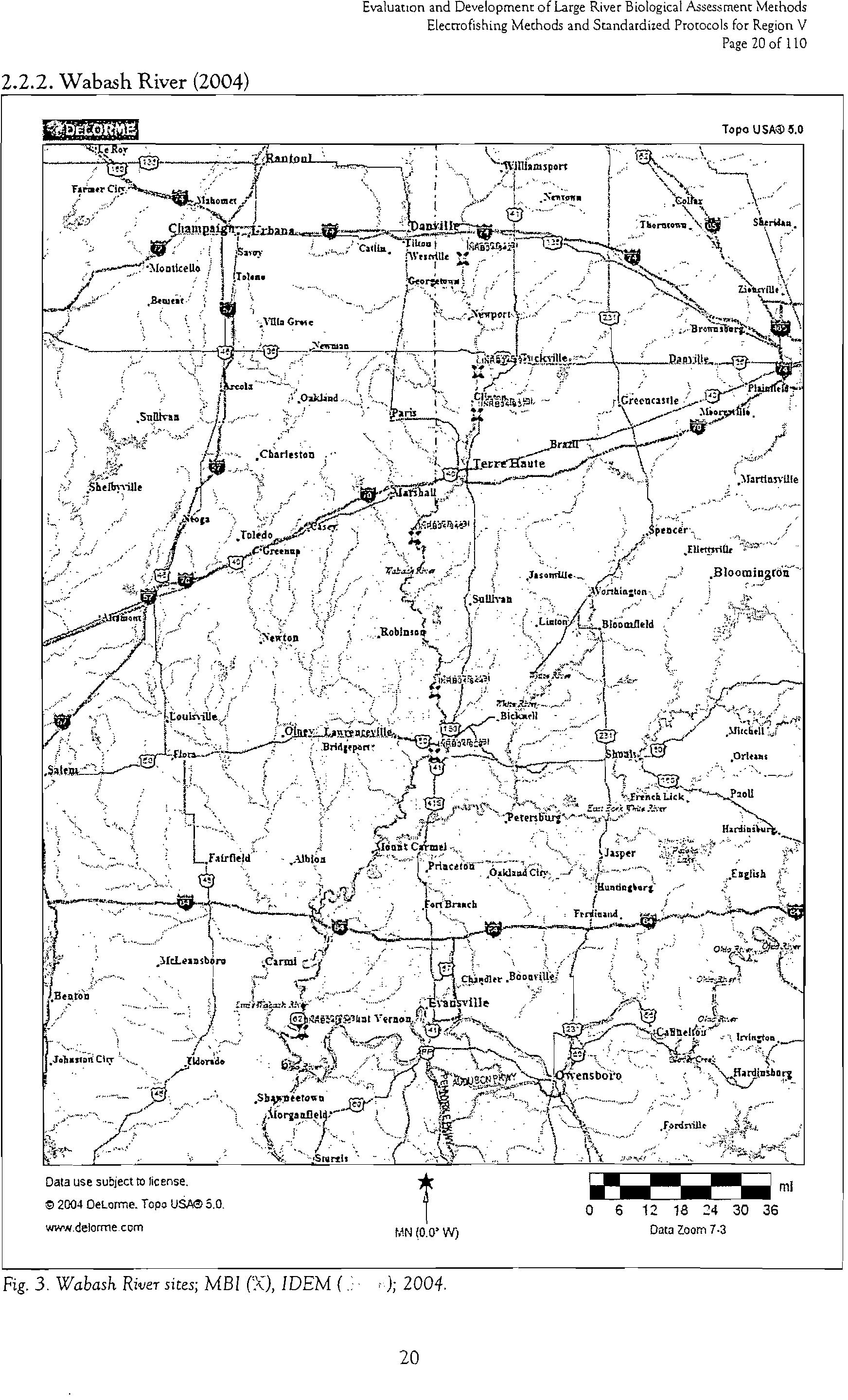
2.2.2. Wabash River
20
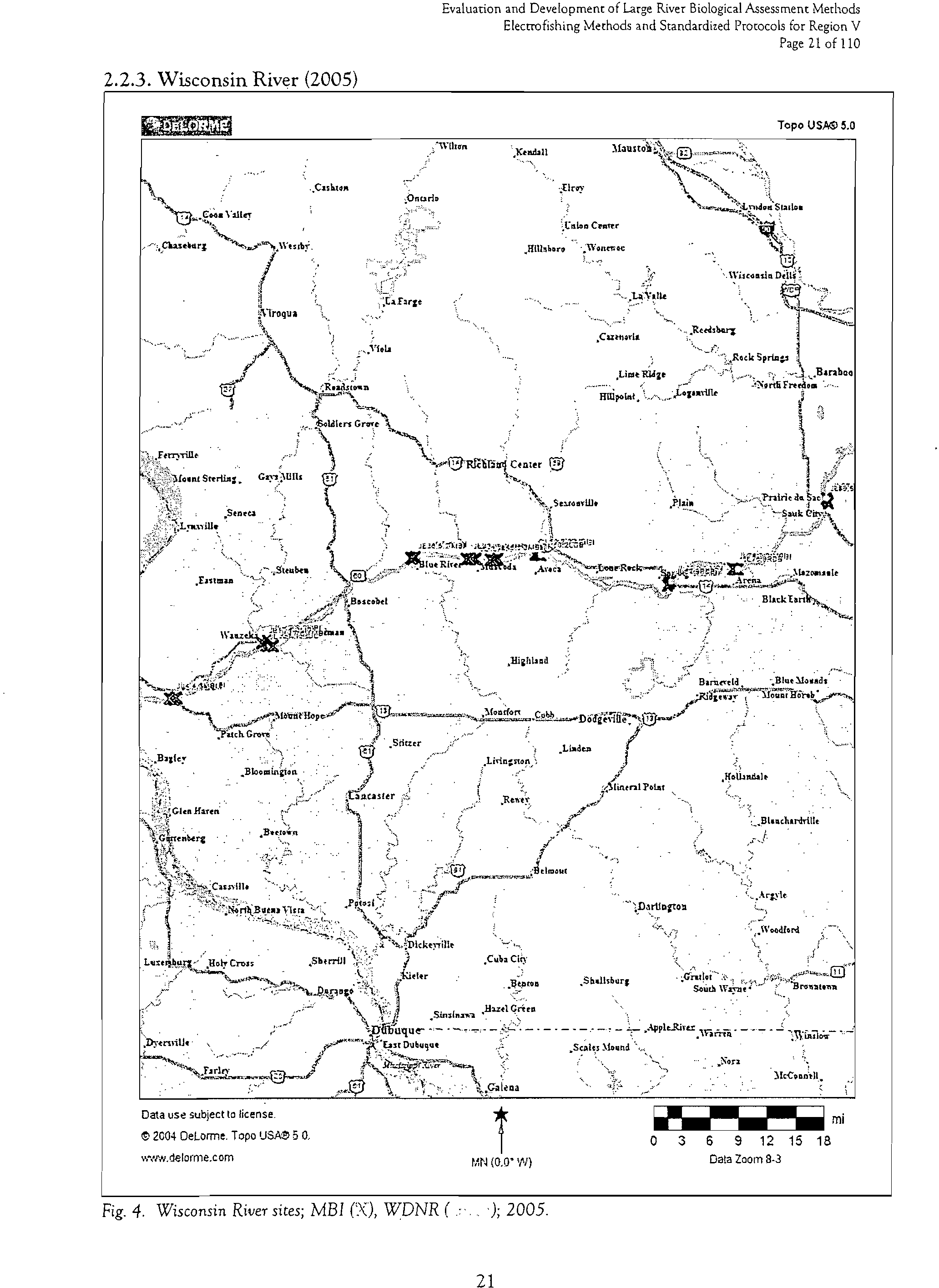
2.2.3. Wisconsin River
21
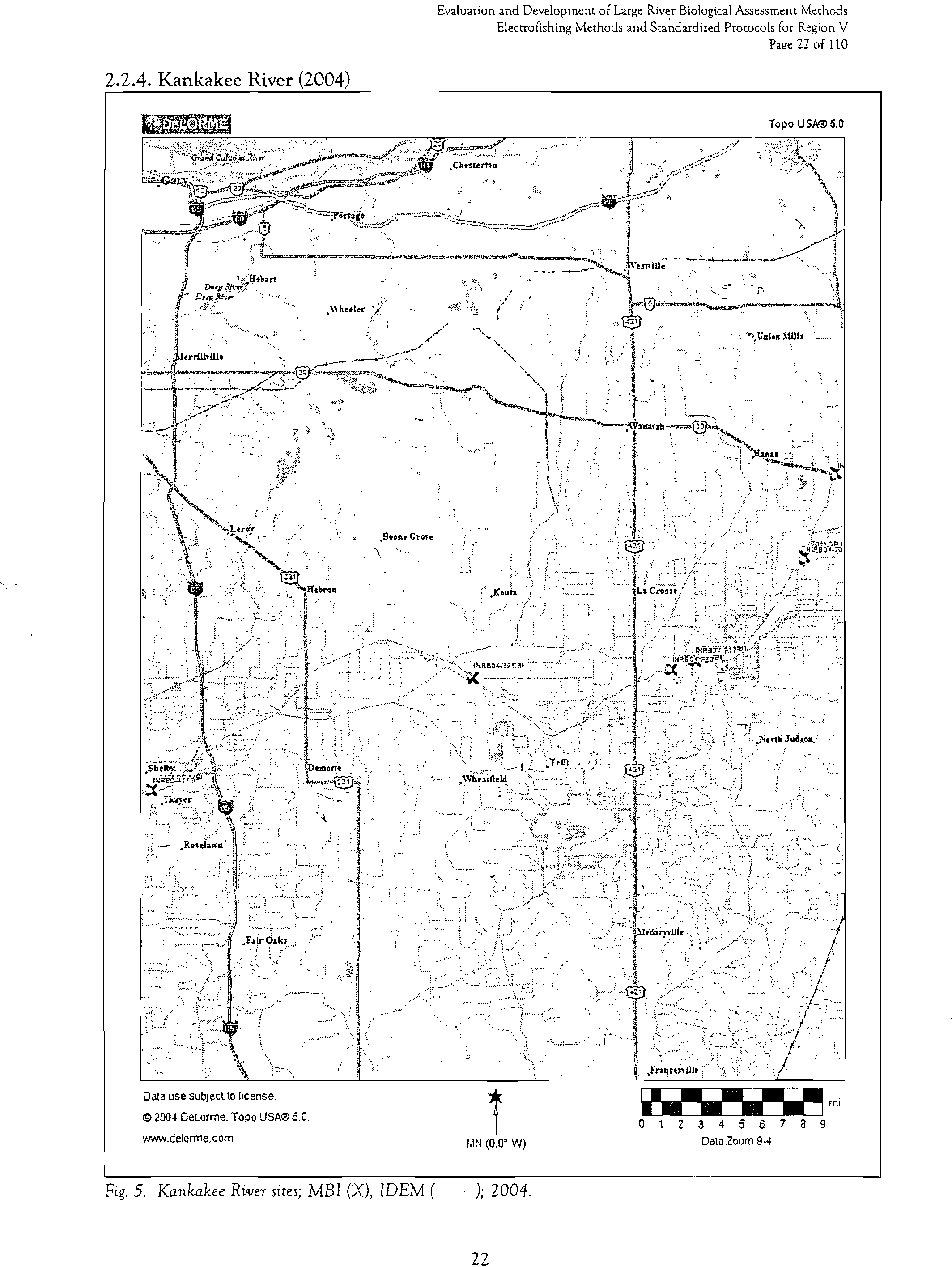
2.2.4. Kankakee River (2004)
22
2.2.5. Kankakee River (2005)
23
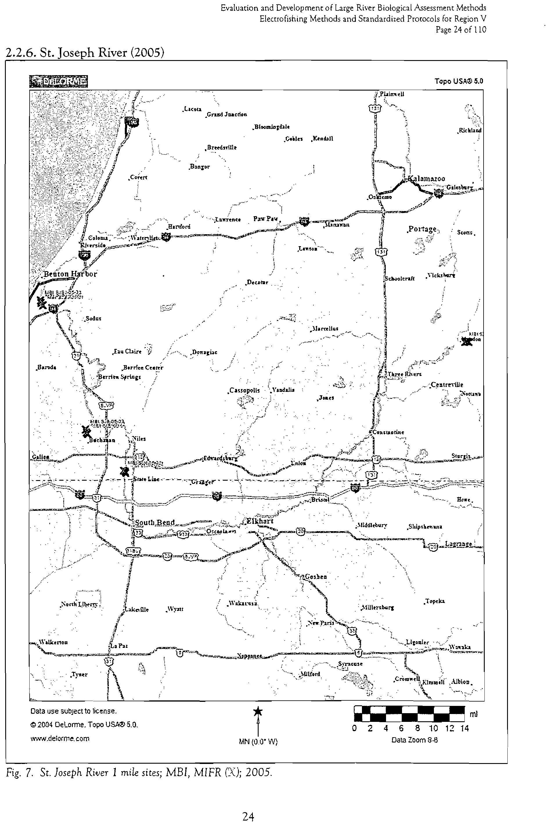
2.2.6. St Joseph River; 1 Mile sites
24
2.2.6. St Joseph River; 500m sites
25
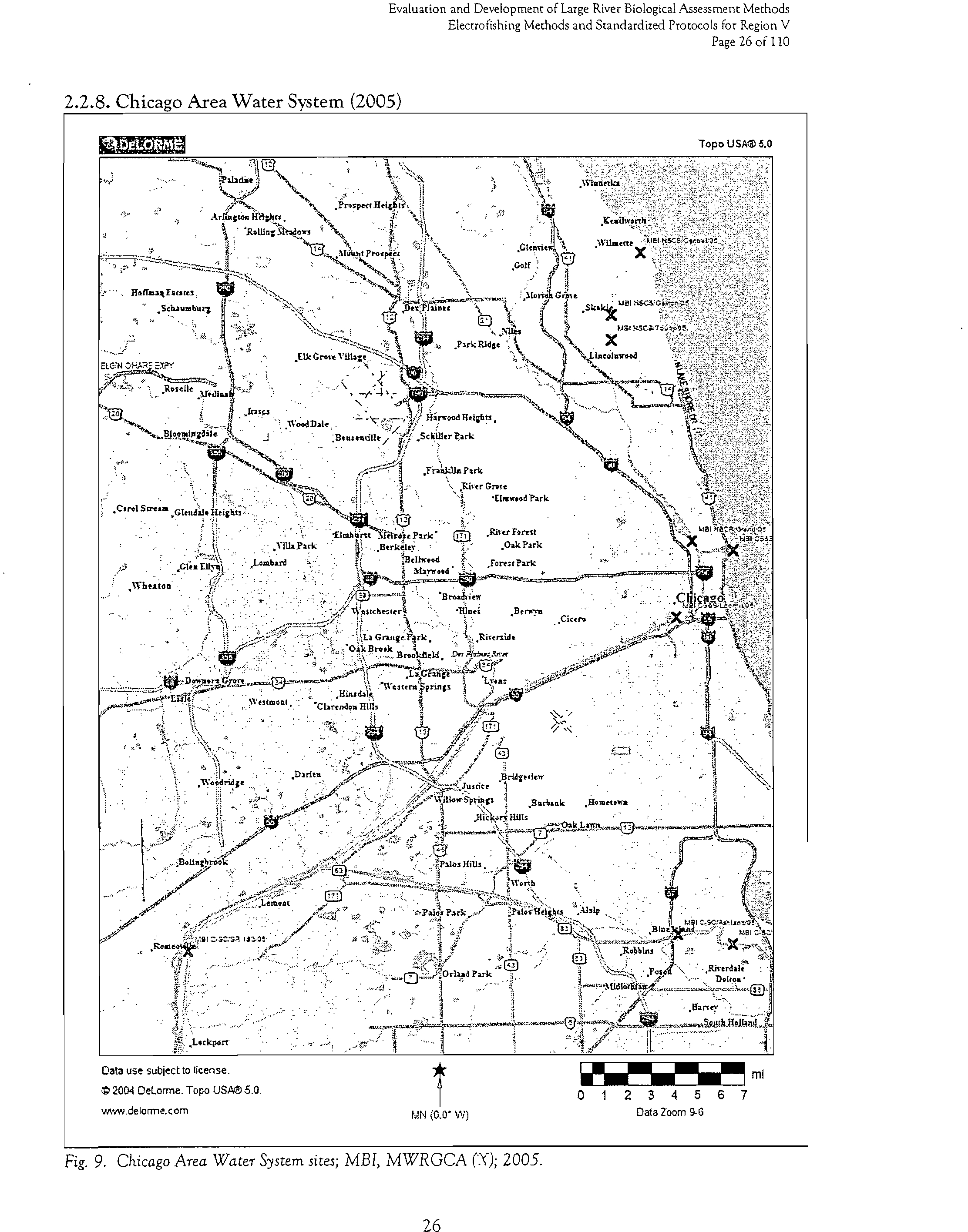
2.2.8. Chicago Area Water System (CAWS)
26
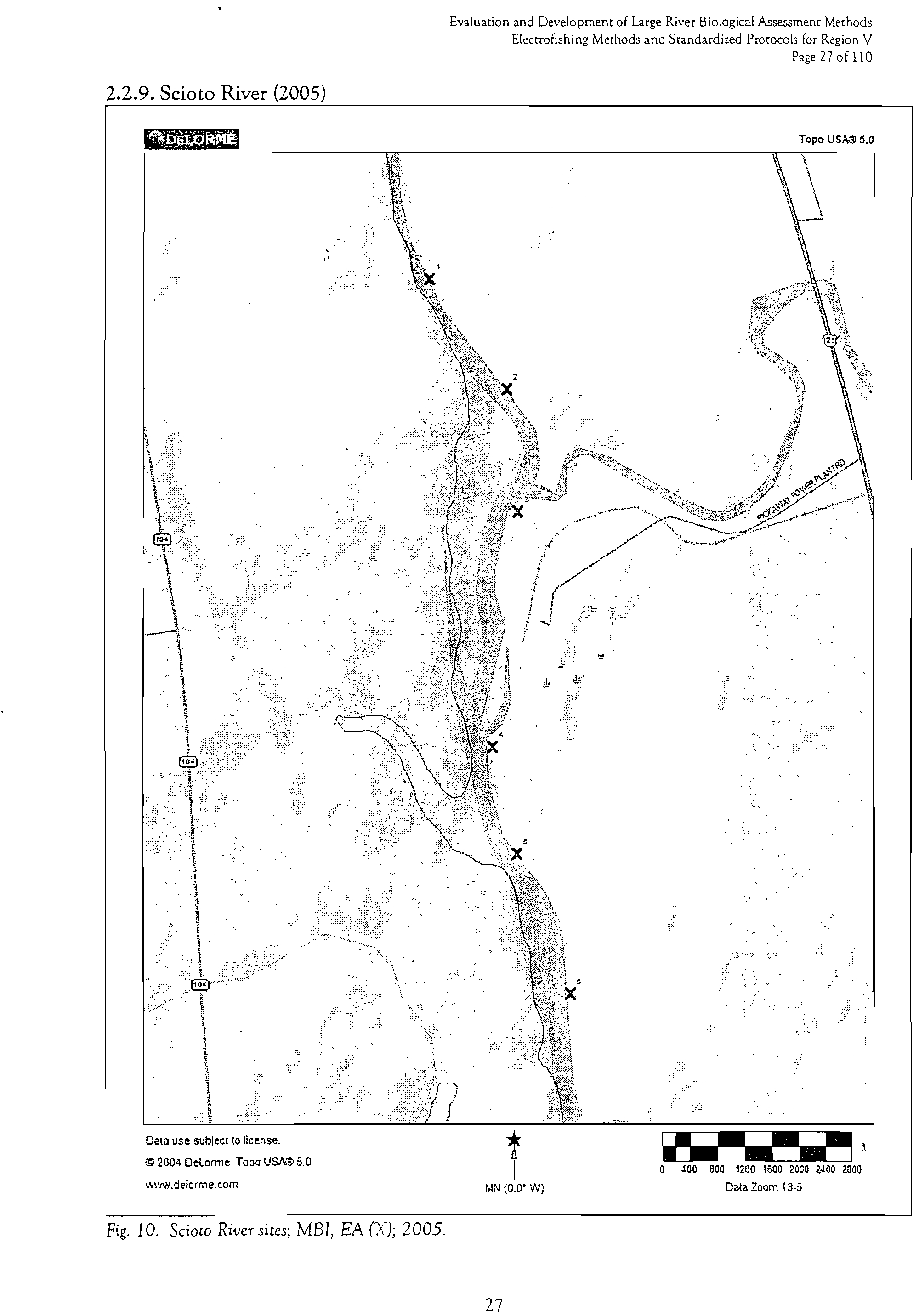
2.2.9. Scioto River
27
2.3. Sampling Equipment/ Protocols
28
2.3.1. Midwest Biodiversity Institute
28
2.3.2. Minnesota DNR
32
2.3.3. Minnesota PCA
33
2.3.4. Indiana DEM
34
2.3.5. Wisconsin DNR
35
2.3.6. Illinois DNR
36
2.3.7. Michigan Institute for Fisheries Research
36
2.3.8. City of Elkhart
37
2.3.9. Metropolitan Water Reclamation District Greater Chicago
37
2.3.10. American Electric Power
38
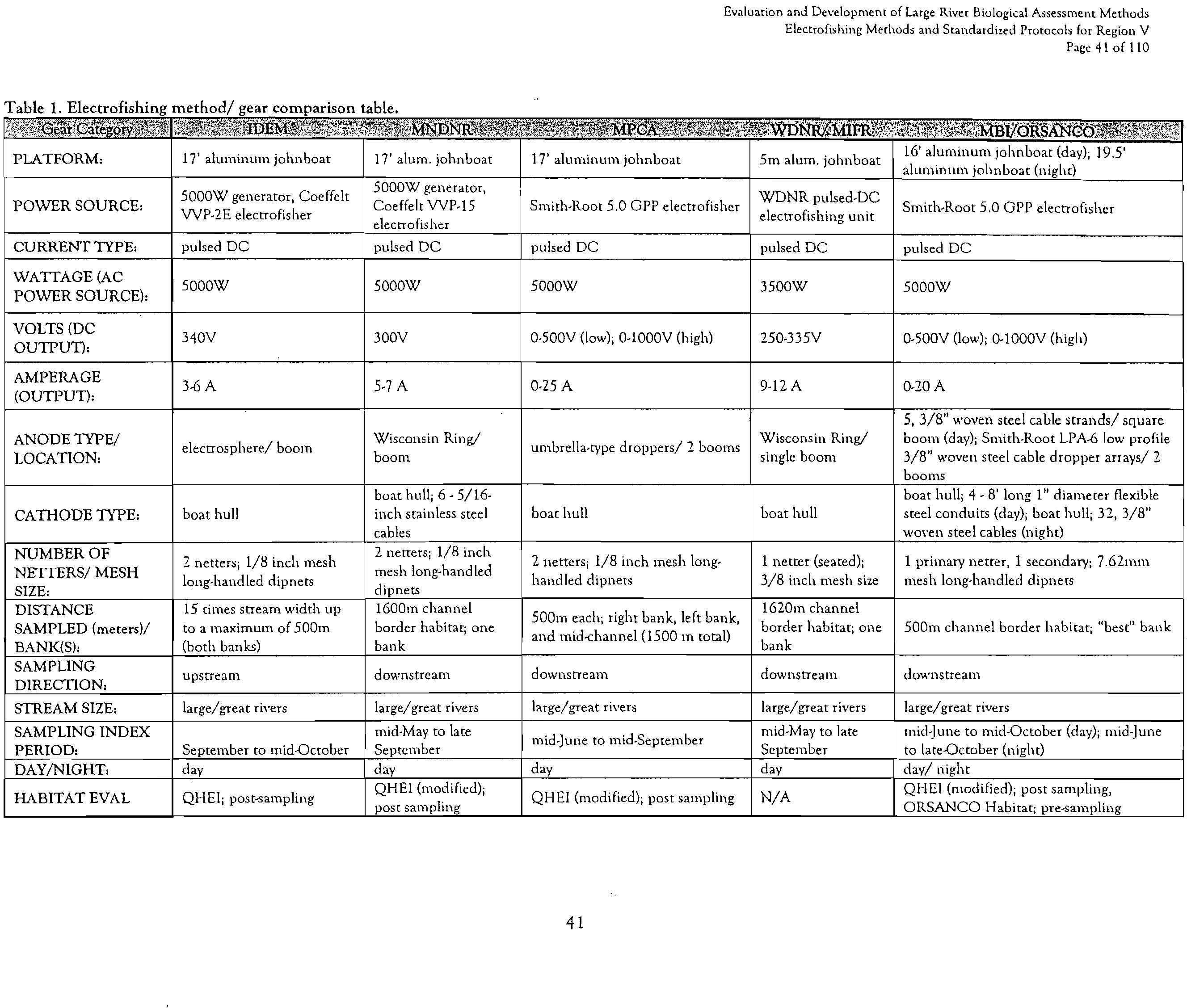
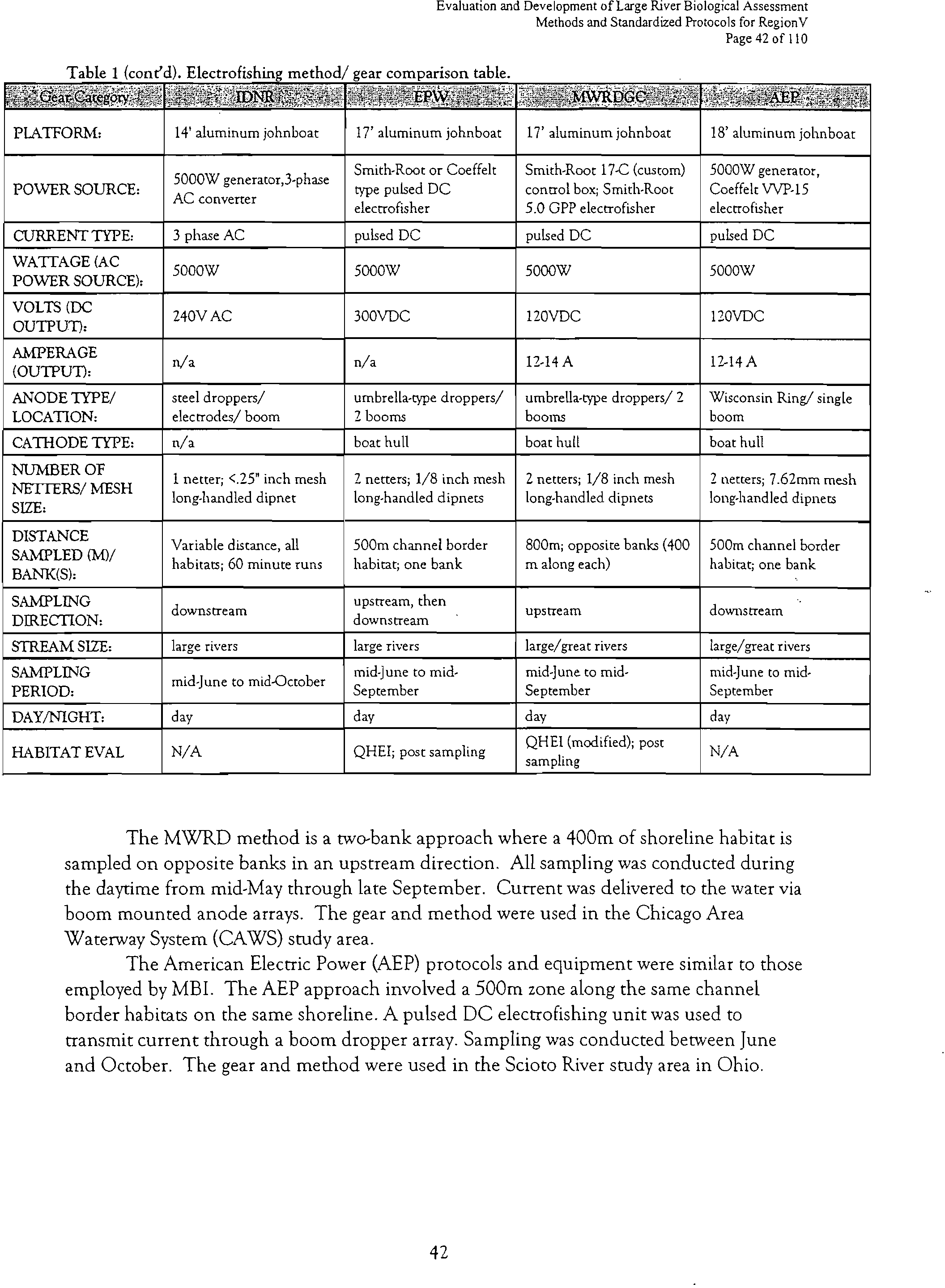
2.3.11. Principal Differences (Electrofishing Method Summary)
39
2.4. Analytical Methods
43
2.4.1. Data Compilation
43
2
Evaluation and Development of Large River Biological Assessment Methods
Electrofishing Methods and Standardized Protocols for Region V
Page 3 of 110
2.4.2. Data Analysis
?
43
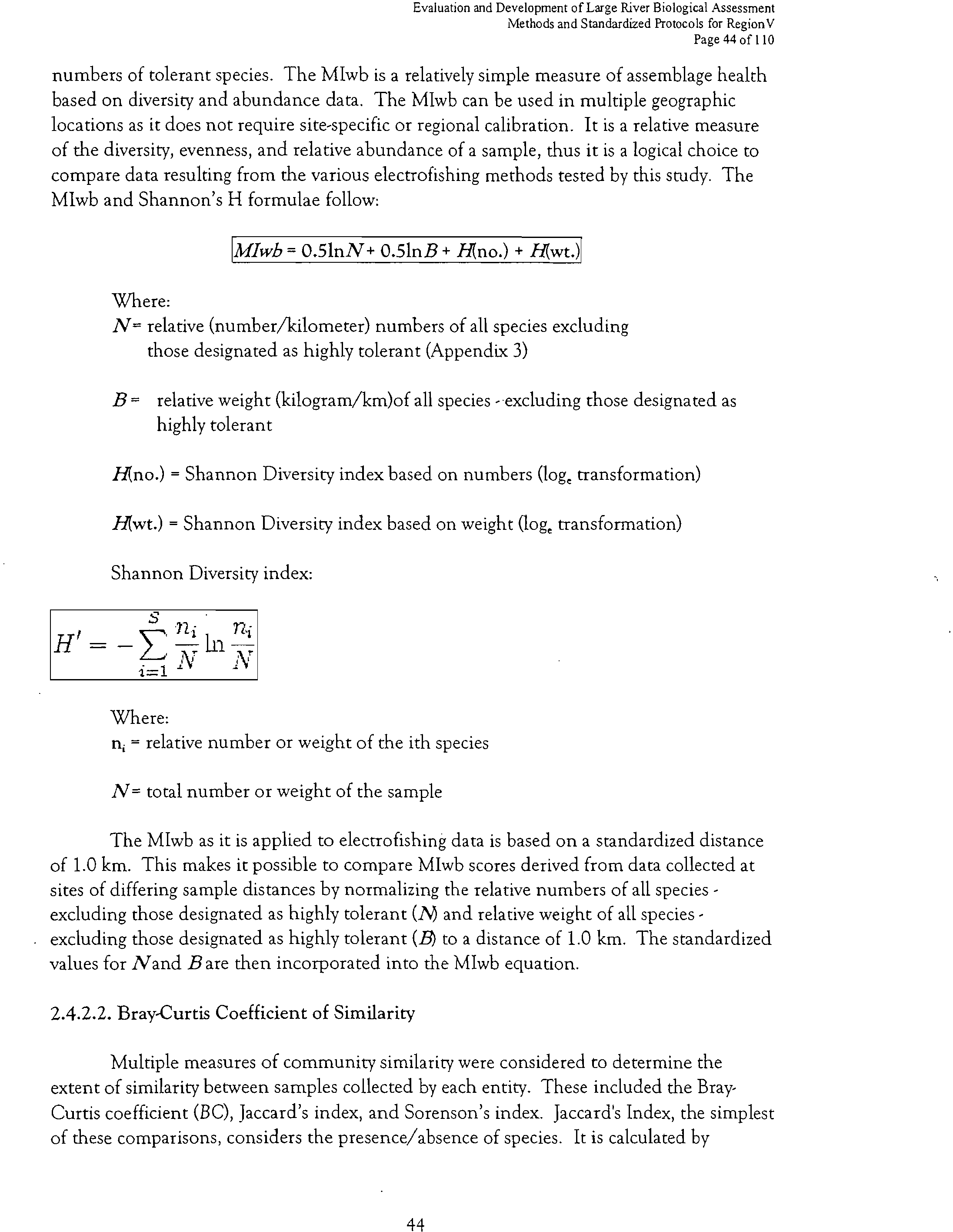
2.4.2.1. Modified Index of Well Being (MIwb)
?
43
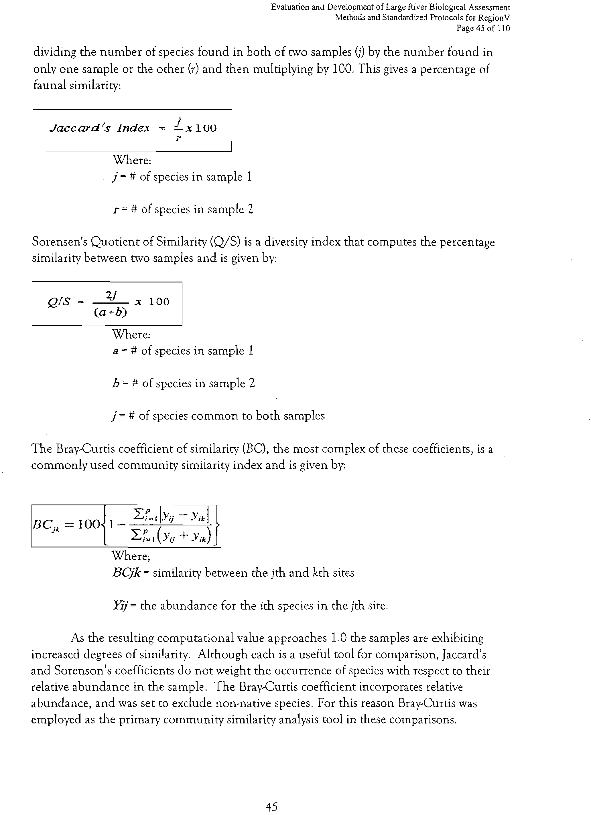
2.4.2.2. Bray-Curtis Coefficient of Community Similarity
?
44
2.4.2.3. Establishing Normal Variation in Assemblage Parameters
?
46
3. RESULTS
3.1. St. Croix River
?
49
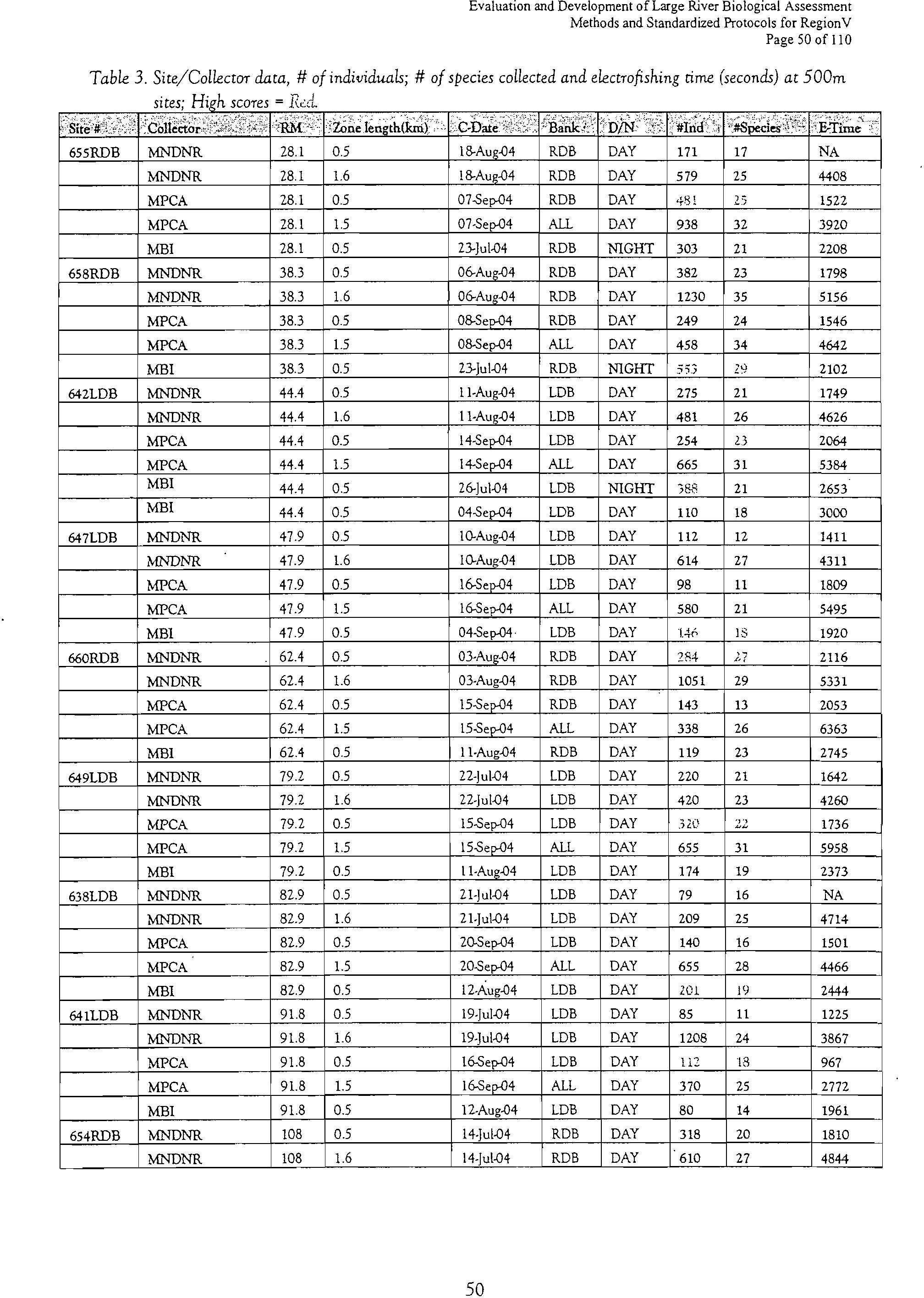
3.1.1. Species Composition / Metrics; #species, #individuals, electrofishing
time per site (10)
?
49
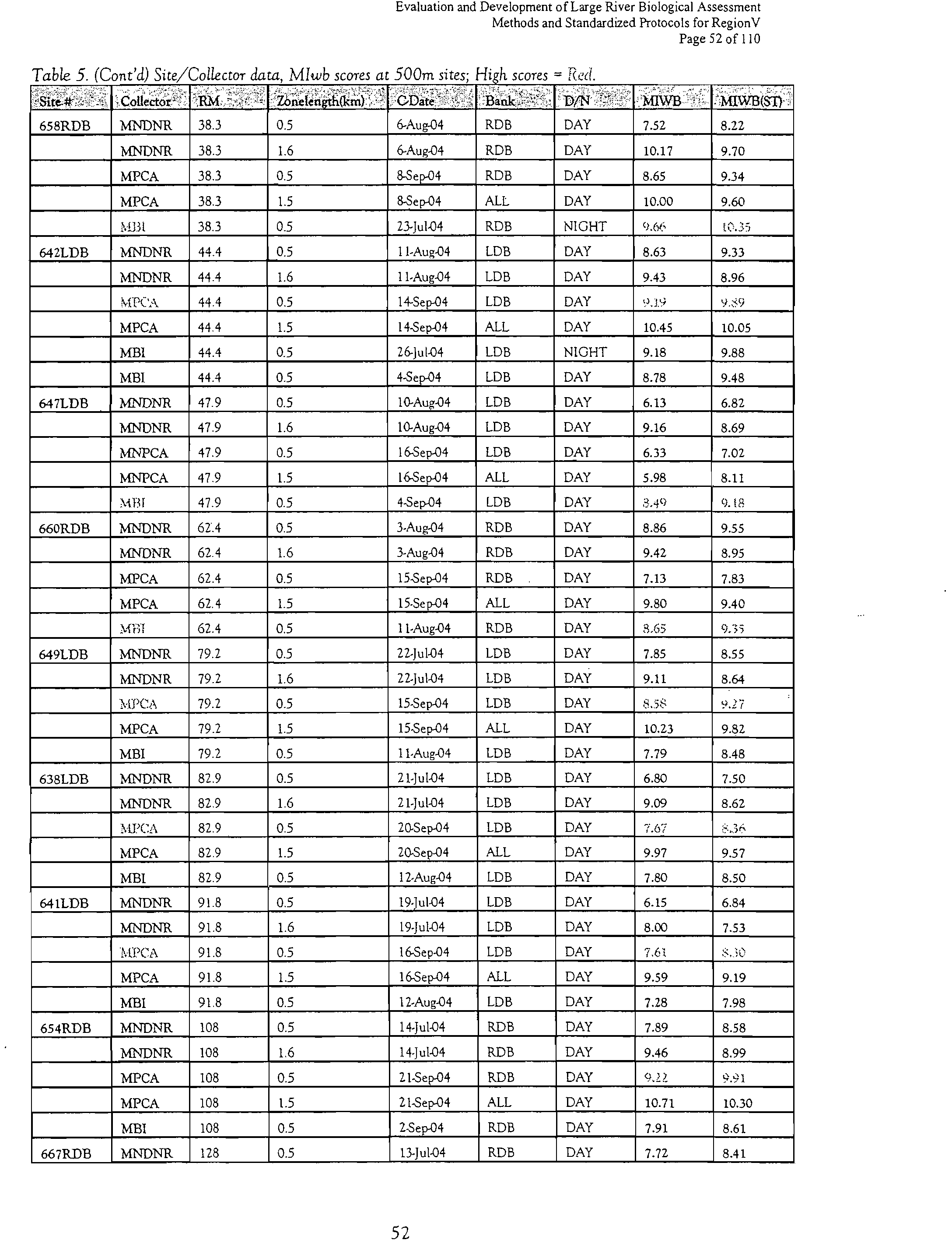
3.1.2. Mlwb Scores ?
51
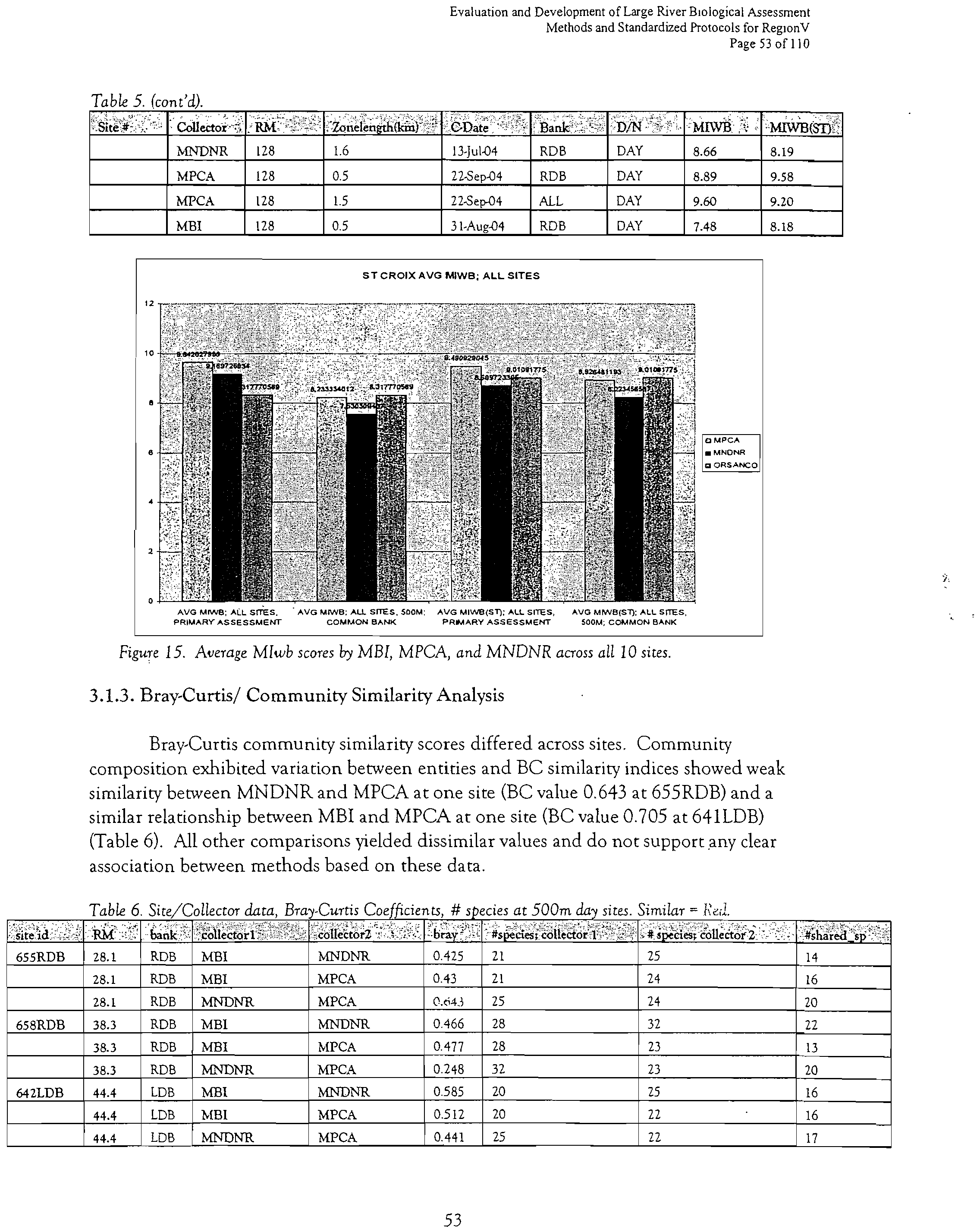
3.1.3. Bray-Curtis/ Community Similarity Analysis
?
53
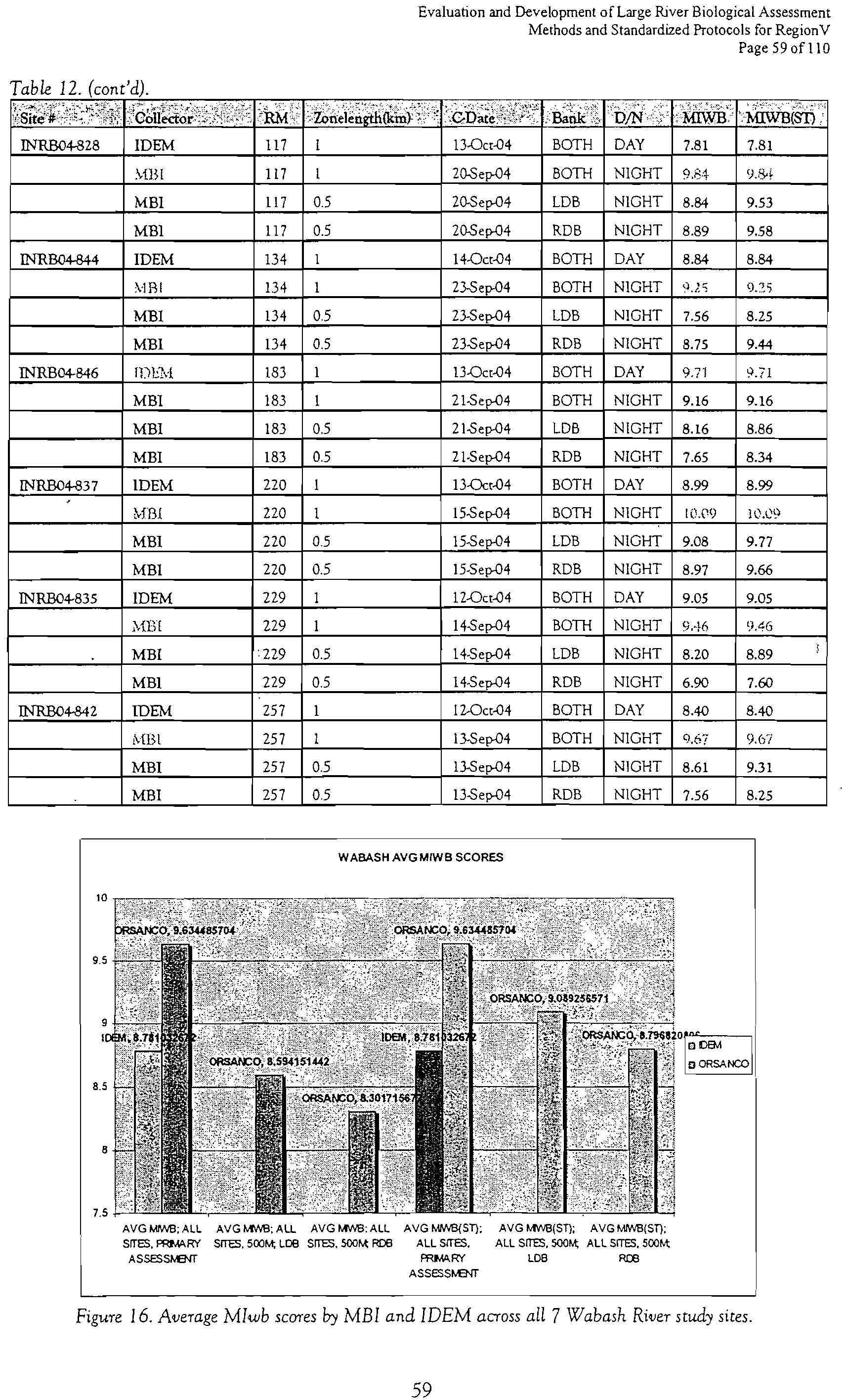
3.2. Wabash River ?
57
3.2.1. Species Composition / Metrics; #species, #individuals, electrofishing
time ?
57
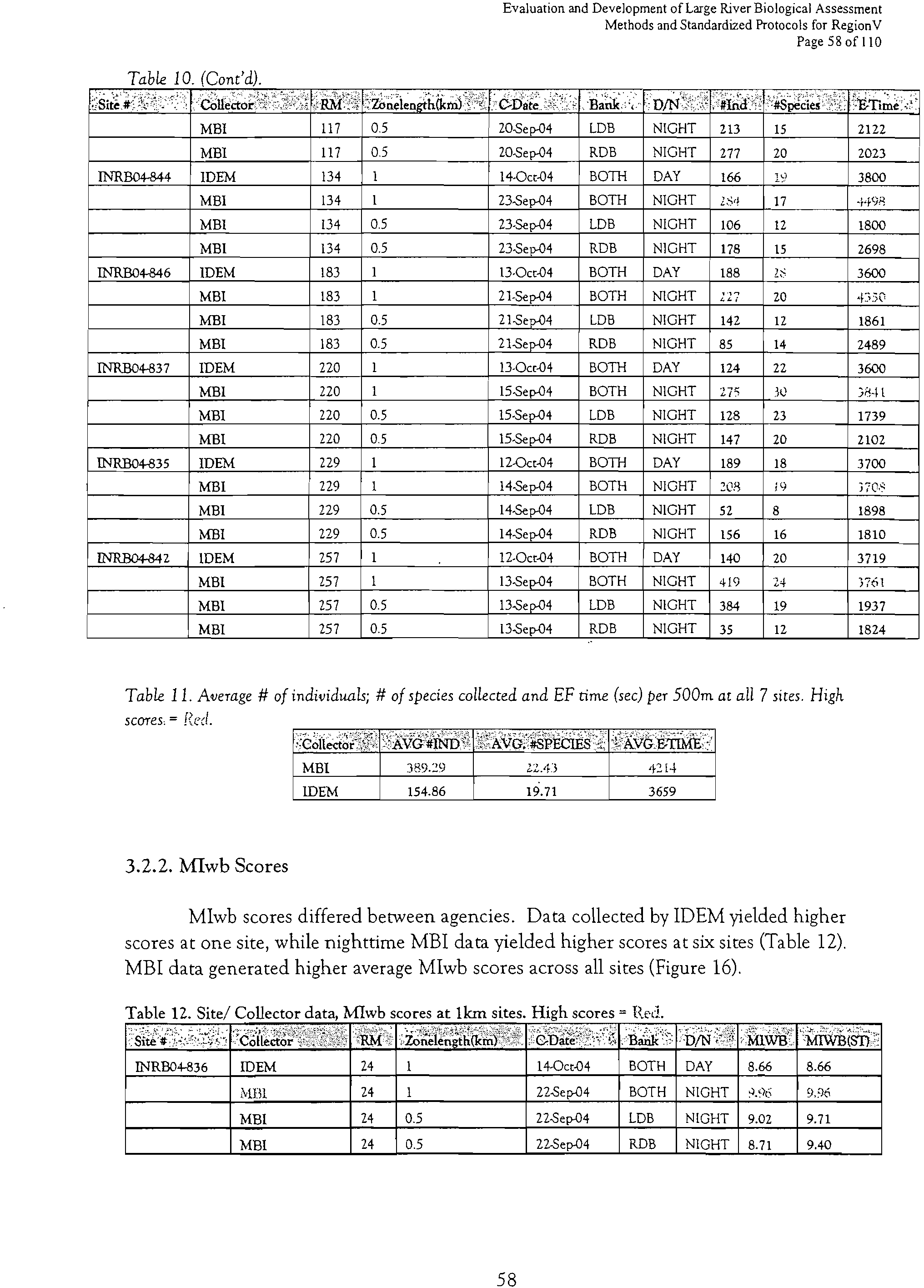
3.2.2. Mlwb Scores
?
58
3.2.3. Bray-Curtis/ Community Similarity Analysis
?
60
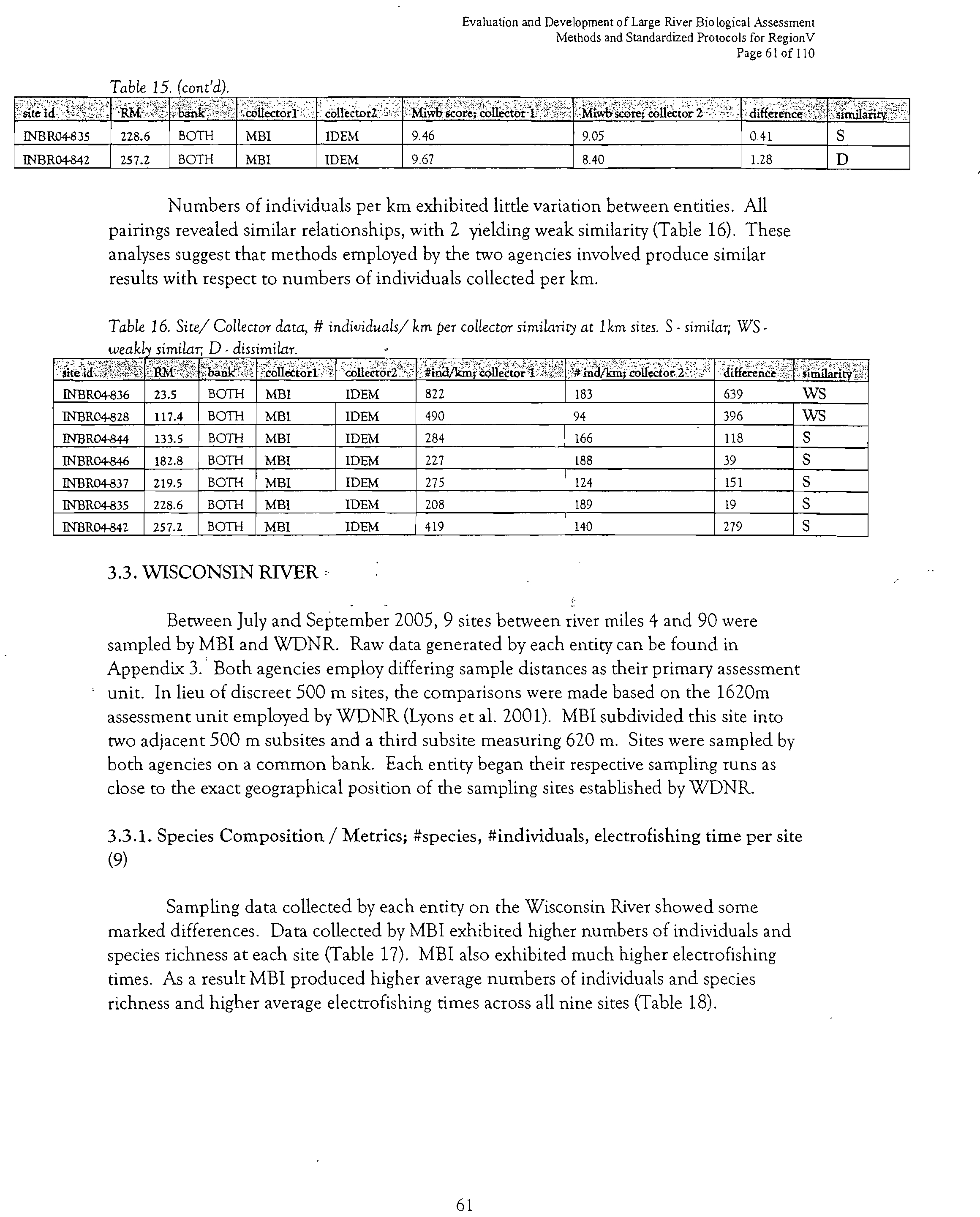
3.3. Wisconsin River ?
61
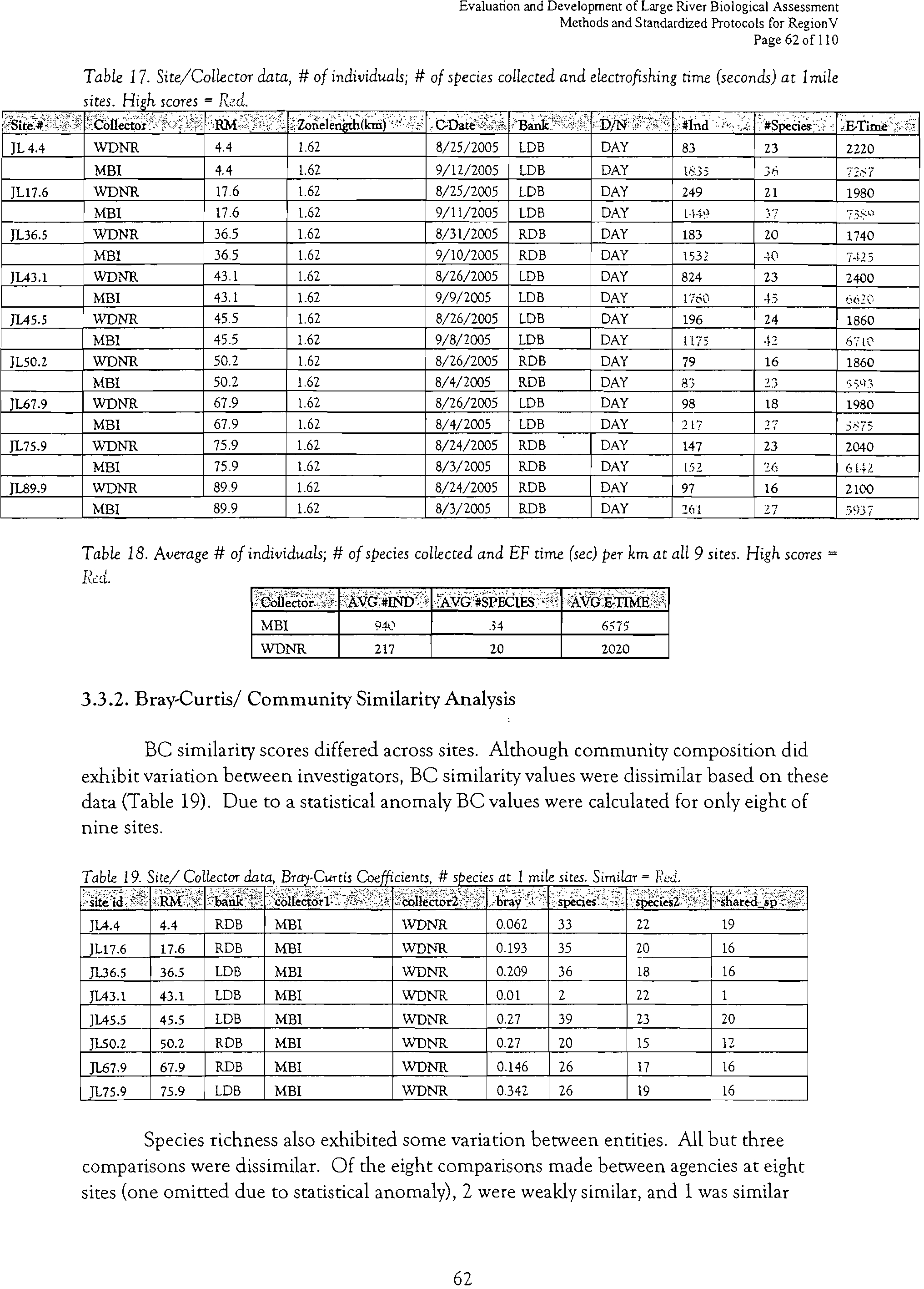
3.3.1. Species Composition / Metrics; #species, #individuals, electrofishing
time
?
61
3.3.2. MIwb Scores ?
62
3.3.3. Bray-Curtis/ Community Similarity Analysis
?
63
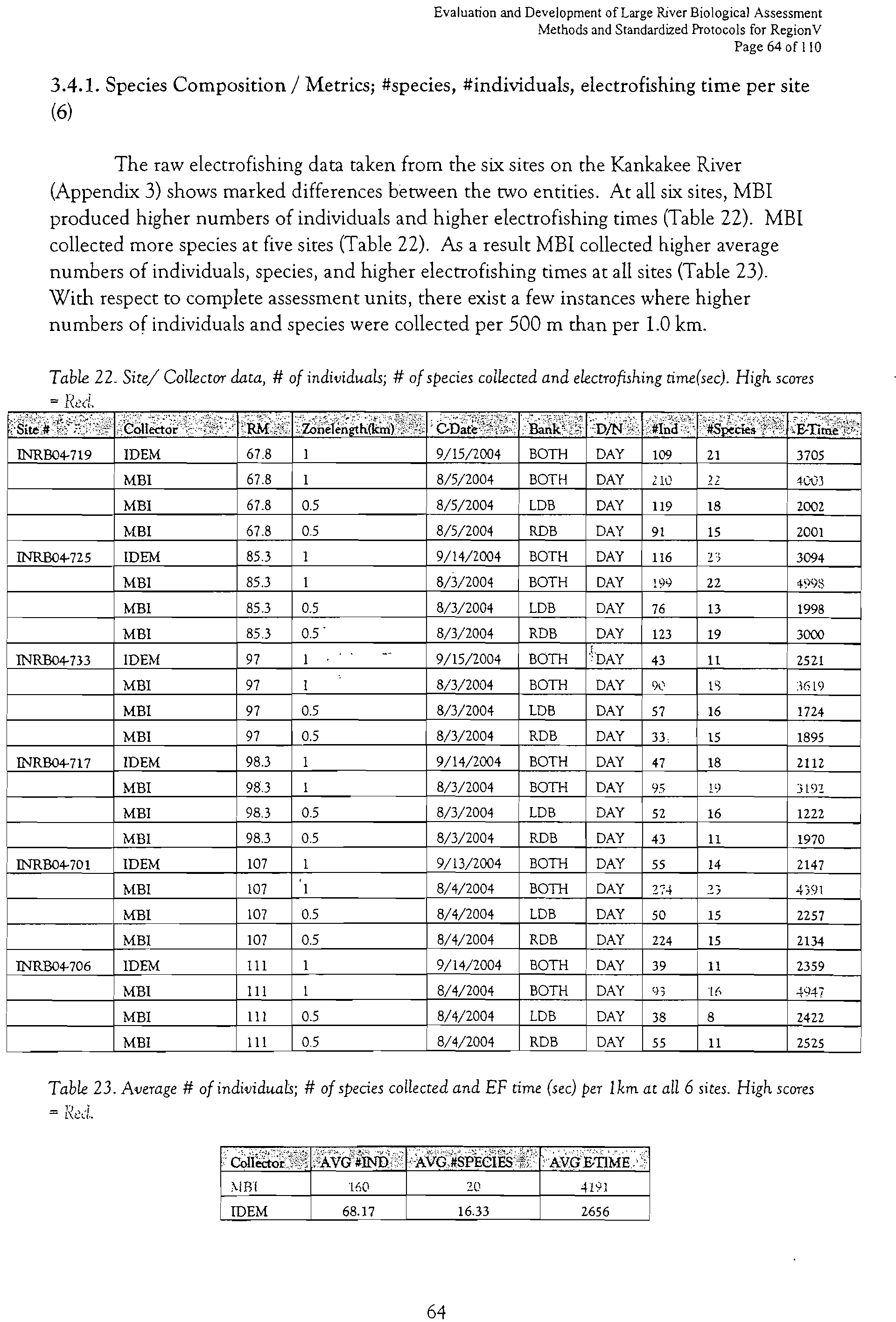
3.4. Kankakee River (2004)
?
64
3.4:1. Species Composition / Metrics; #species, #individuals, electrofishing
time
?
?
64
3.4.2. MIwb Scores
?
65
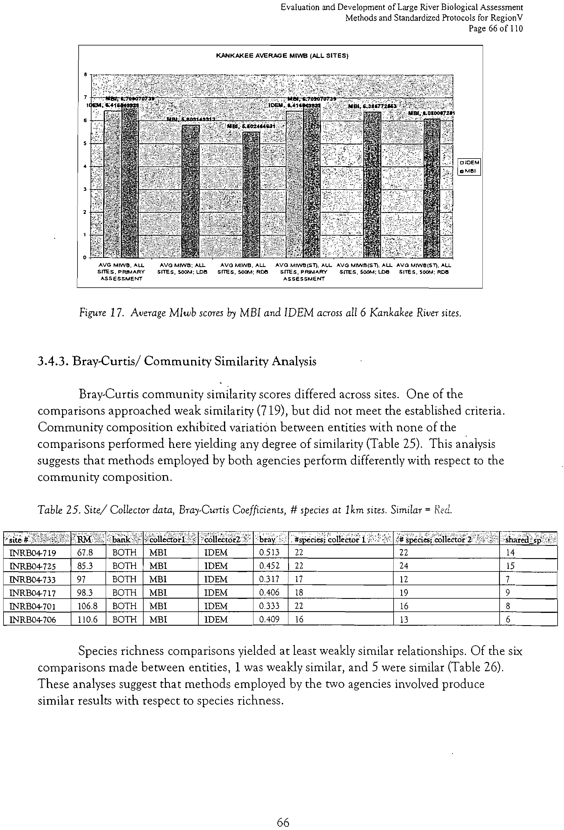
3.4.3. Bray-Curtis/ Community Similarity Analysis
?
66
3.5. Kankakee River (2005) ?
68
3.5.1. Species Composition / Metrics; #species, #individuals, electrofishing
time
?
68
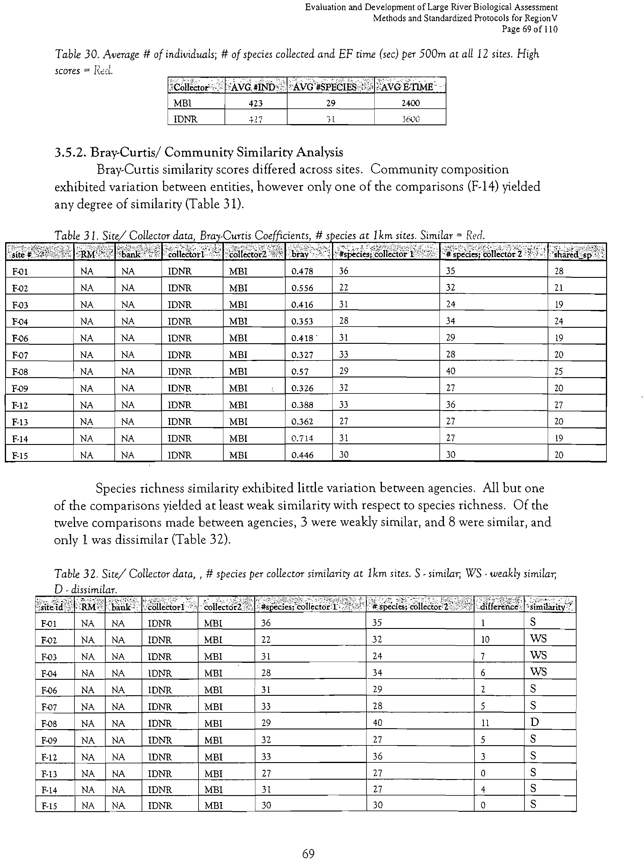
3.5.2. Bray-Curtis/ Community Similarity Analysis
?
69
3.6. St Joseph River (Indiana)
?
71
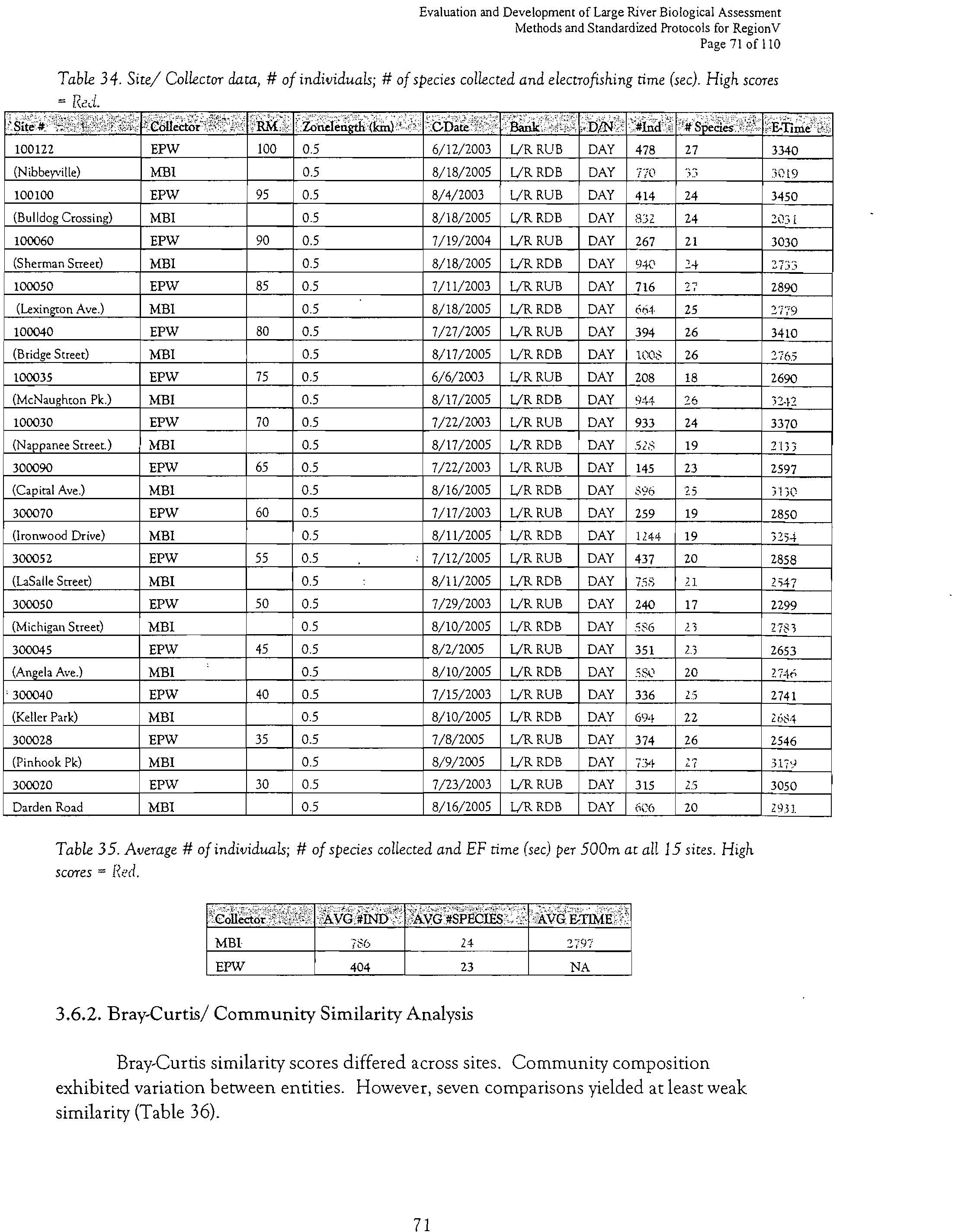
3.6.1. Species Composition / Metrics; #species, #individuals, electrofishing
time
?
71
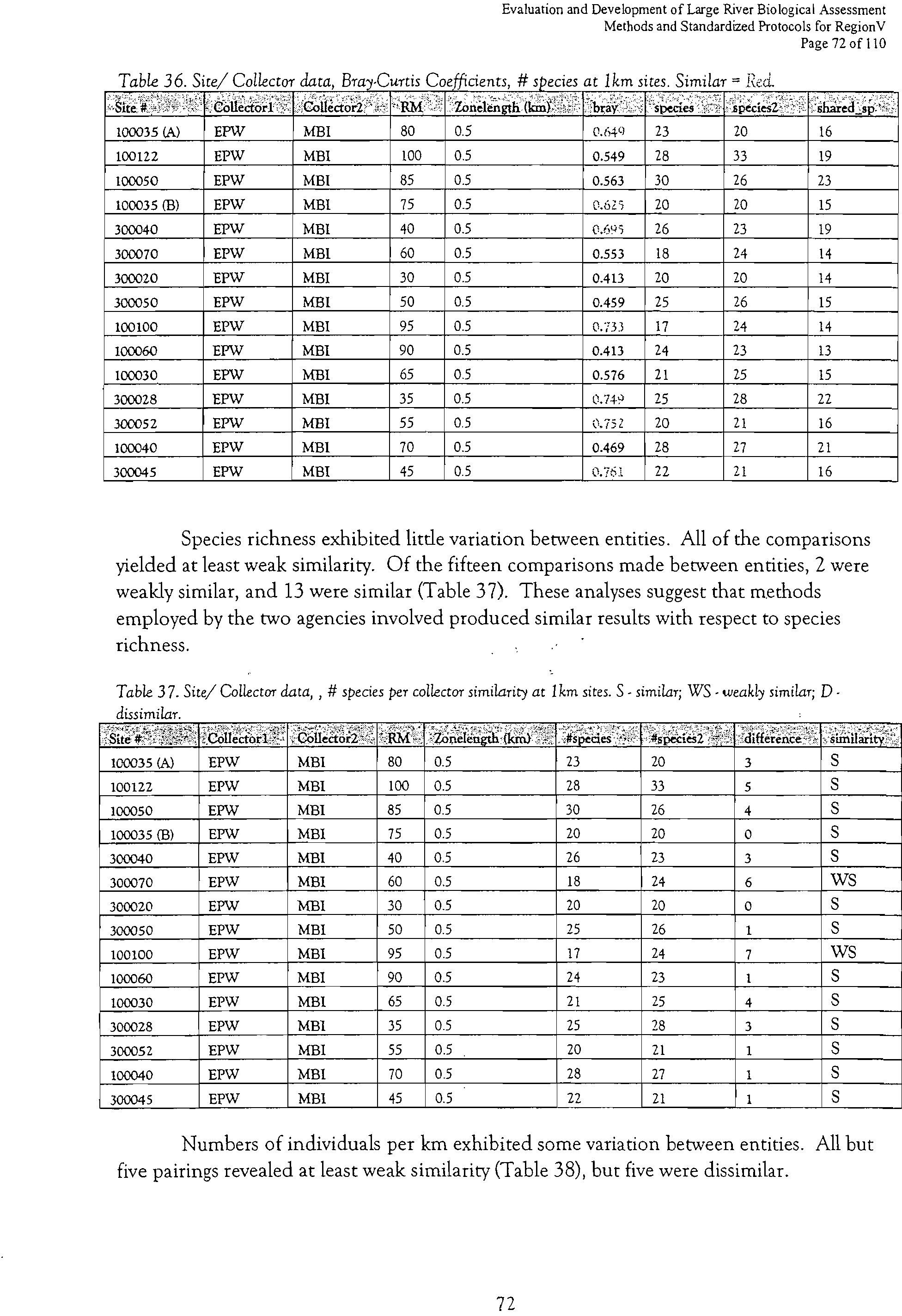
3.6.2. Bray-Curtis/ Community Similarity Analysis
?
72
3.7. St Joseph River (Michigan)
?
74
3.7.1. Species Composition / Metrics; #species, #individuals, electrofishing
time
?
74
3.7.2. Bray-Curtis/ Community Similarity Analysis
?
74
3.8. Chicago Area Water System (CAWS)
?
75
3.8.1. Species Composition / Metrics; #species, #individuals, electrofishing
time
?
75
3.8.2. Bray-Curtis/ Community Similarity Analysis
?
76
3.9. Scioto River
?
77
3
Evaluation and Development of Large River Biological Assessment Methods
Electrofishing Methods and Standardized Protocols for Region V
Page 4 of 110
3.9.1. Species Composition / Metrics; #species, #individuals, electrofishing
time per site (6) ?
77
3.9.2. Bray-Curtis/ Community Similarity Analysis ?
78
4. DISCUSSION
4.1. St. Croix River
?
81
4.2. Wabash River
?
84
4.3. Wisconsin River ?
87
4.4. Kankakee River (2004)
?
89
4.5. Kankakee River (2005)
?
90
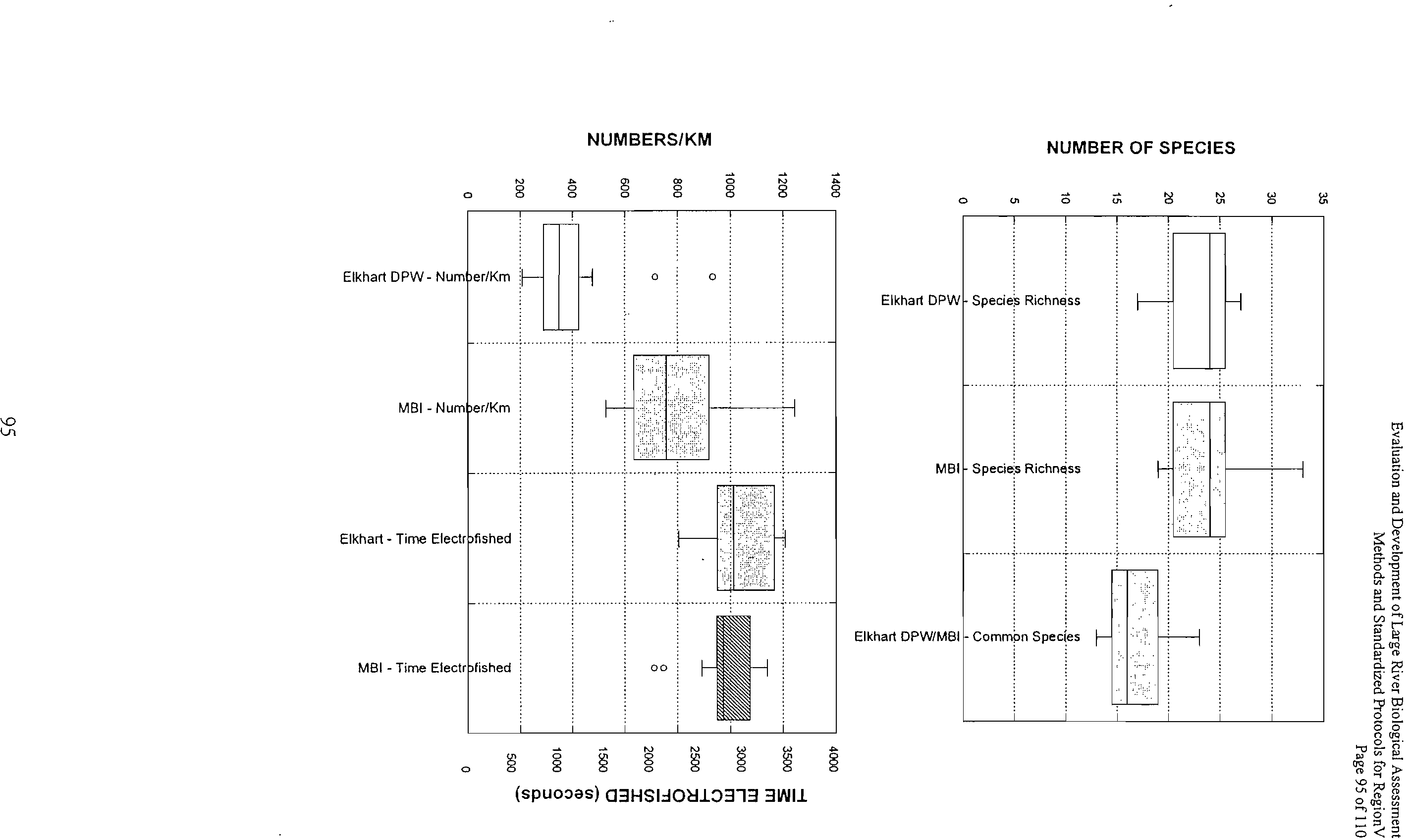
4.6. St Joseph River (Indiana) ?
94
4.7. St Joseph River (Michigan)
?
96
4.8. Chicago Area Water System (CAWS) ?
96
4.9. Scioto River ?
98
5.
SYNTHESIS OF RESULTS ?
102
6. REFERENCES
?
105
ACKNOWLEDGEMENTS
This study was made possible by the cooperation of the organizations and individuals who
agreed to participate by providing sampling effort, data, logistical support, and report
review. This includes the following organizations and personnel: Minnesota PCA (Dan
Helwig, Scott Niemela, Mike Feist), Minnesota DNR (Nick Proulx), Wisconsin DNR (John
Lyons), Illinois DNR (Steve Pescitelli), Indiana DEM (Stacey Sobat), Elkhart Department
of Public Works (Len Kring, Joe Foy), Metropolitan Water Reclamation District of Greater
Chicago (Jennifer Wasik, Sam Denison), Michigan DNR/IFR (Dana Infante), and
American Electric Power (Alan Gaulke). This study would not have been possible without
the direct participation and cooperation of these organizations and individuals. Ed
Hammer, U.S. EPA, Region V provided technical assistance and project oversight.
Funding for this study was provided by U.S. EPA, Region V under Section 104(b)(3) of the
Clean Water Act via grant CP-96510501.
4
Evaluation and Development of Large River Biological Assessment Methods
Electrofishing Methods and Standardized Protocols for Region V
Page 5 of 110
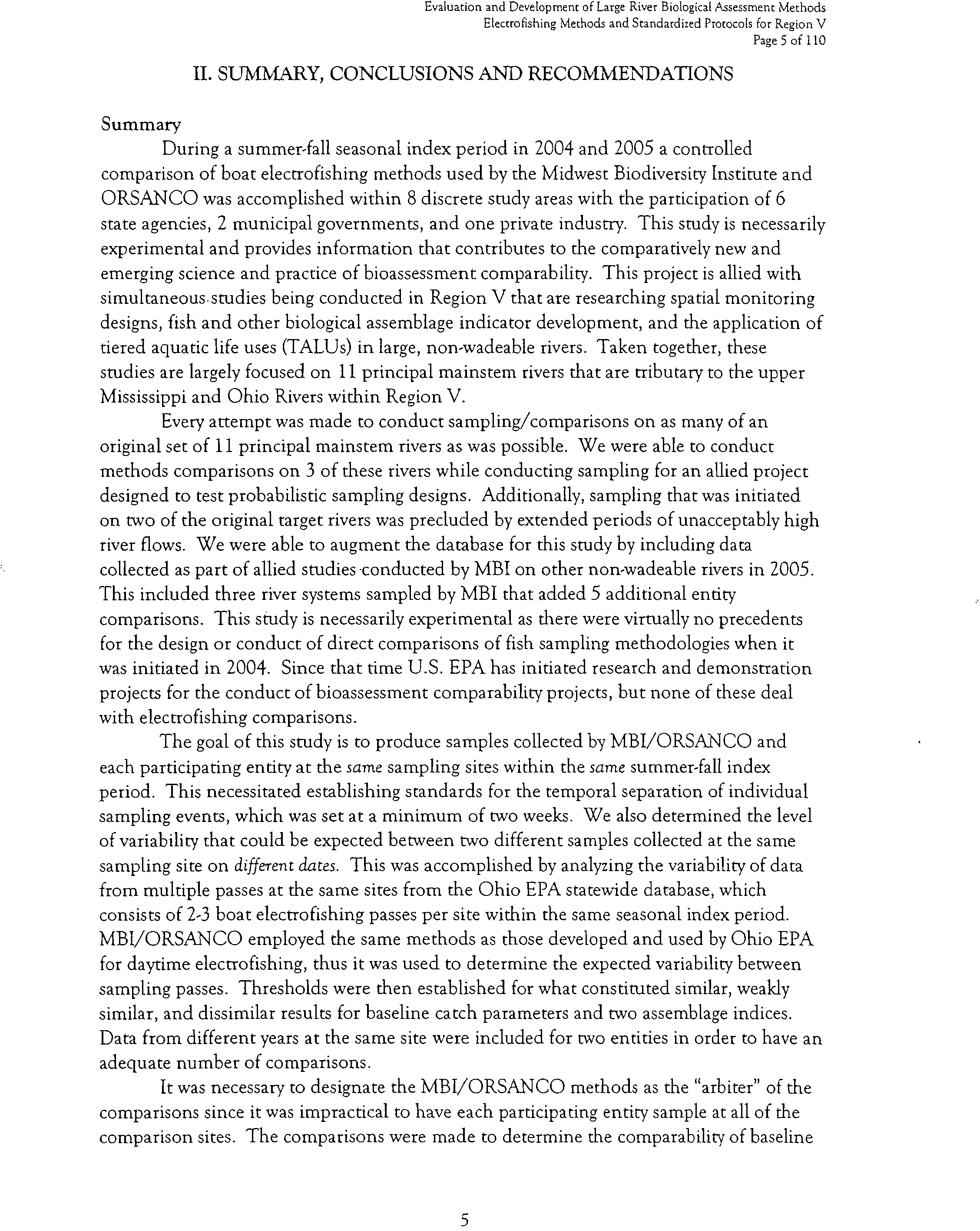
II. SUMMARY, CONCLUSIONS AND RECOMMENDATIONS
Summary
During a summer-fall seasonal index period in 2004 and 2005 a controlled
comparison of boat electrofishing methods used by the Midwest Biodiversity Institute and
ORSANCO was accomplished within 8 discrete study areas with the participation of 6
state agencies, 2 municipal governments, and one private industry. This study is necessarily
experimental and provides information that contributes to the comparatively new and
emerging science and practice of bioassessment comparability. This project is allied with
simultaneous.studies being conducted in Region V that are researching spatial monitoring
designs, fish and other biological assemblage indicator development, and the application of
tiered aquatic life uses (TALUs) in large, non-wadeable rivers. Taken together, these
studies are largely focused on 11 principal mainstem rivers that are tributary to the upper
Mississippi and Ohio Rivers within Region V.
Every attempt was made to conduct sampling/comparisons on as many of an
original set of 11 principal mainstem rivers as was possible. We were able to conduct
methods comparisons on 3 of these rivers while conducting sampling for an allied project
designed to test probabilistic sampling designs. Additionally, sampling that was initiated
on two of the original target rivers was precluded by extended periods of unacceptably high
river flows. We were able to augment the database for this study by including data
collected as part of allied studies -conducted by MBI on other non-wadeable rivers in 2005.
This included three river systems sampled by MBI that added 5 additional entity
comparisons. This study is necessarily experimental as there were virtually no precedents
for the design or conduct of direct comparisons of fish sampling methodologies when it
was initiated in 2004. Since that time U.S. EPA has initiated research and demonstration
projects for the conduct of bioassessment comparability projects, but none of these deal
with electrofishing comparisons.
The goal of this study is to produce samples collected by MBI/ORSANCO and
each participating entity at the
same
sampling sites within the
same
summer-fall index
period. This necessitated establishing standards for the temporal separation of individual
sampling events, which was set at a minimum of two weeks. We also determined the level
of variability that could be expected between two different samples collected at the same
sampling site on
different dates.
This was accomplished by analyzing the variability of data
from multiple passes at the same sites from the Ohio EPA statewide database, which
consists of 2-3 boat electrofishing passes per site within the same seasonal index period.
MBI/ORSANCO employed the same methods as those developed and used by Ohio EPA
for daytime electrofishing, thus it was used to determine the expected variability between
sampling passes. Thresholds were then established for what constituted similar, weakly
similar, and dissimilar results for baseline catch parameters and two assemblage indices.
Data from different years at the same site were included for two entities in order to have an
adequate number of comparisons.
It was necessary to designate the MBI/ORSANCO methods as the "arbiter" of the
comparisons since it was impractical to have each participating entity sample at all of the
comparison sites. The comparisons were made to determine the comparability of baseline
5
Evaluation and Development of Large River Biological Assessment Methods
Electrofishing Methods and Standardized Protocols for Region V
Page 6 of 110
sample parameters such as species richness, relative numbers, and relative biomass. As
such these are the baseline "ingredients" of a fish assemblage assessment regardless of the
techniques used to analyze that data. We are focused here on determining if differences
exist, characterizing their magnitude, and attempting to determine what might be the
sources of variation in the results of a respective methodology and its execution beyond
that expected. We analyzed the Ohio EPA boat electrofishing database to determine the
expected variability between sampling passes conducted at the same site on different dates
within the same summer-fall seasonal index period and the same site sampled in different
years. Some variation in baseline sample parameters (species richness, numbers, biomass)
is to be expected even with the same crew and equipment. Thus making comparisons
between two different entities on different dates had to factor this into the comparison of
results.
The comparisons were made using species richness, relative density (numbers/km),
and biomass (kg/km) when the latter was available. We also used two transformations of
the relative abundance data in the comparison analyses, the Modified Index of Well-Being
(MIwb) and the Bray-Curtis coefficient of similarity. The comparisons were made on a
sampling site basis as an average and as a distribution of data for all sites combined. Each
comparison was designated as being similar, weakly similar, or dissimilar. The criteria for
similar results was the 75
th
percentile of the analysis of the Ohio EPA multiple pass data
used to establish the expected variation in results between different dates within the same
seasonal index period or different years for species richness, density, biomass, and the
MIwb. The 25 th
percentile was used for the Bray-Curtis results as a statistically consistent
threshold for that index. Weakly similar results were between the 75
th
and 95
th
percentiles
(25
th and 5
th
for Bray-Curtis), and dissimilar results were outside of the 95
th
percentile (5th
percentile for Bray-Curtis). Using these criteria reflects an increasing deviation of results
between each comparison to the point where the results are either comparable or not for
bioassessment purposes.
Results and Conclusions
It is clear from the information compiled here that there are a variety of differences
between the boat electrofishing protocols used by the different entities involved in this
study. Some of these are easily distinguished and include sampling distance, sampling
direction (upstream vs. downstream), site location (single bank, both banks, mid-channel),
equipment specifications (pulsator specifications, settings, dip net mesh size), number of
netters (1 vs. 2 primary netters, assist netters), and time electrofished. Other differences
were not as apparent, but can be inferred from other information and include the
"thoroughness" of sampling, i.e., how thoroughly were all available habitats (e.g., woody
debris, riffles, gravel shoals, deep runs, pools, all cover types, etc.) sampled. This may be
one of the most important, yet difficult to document variables that contributed to some of
the observed differences in the results.
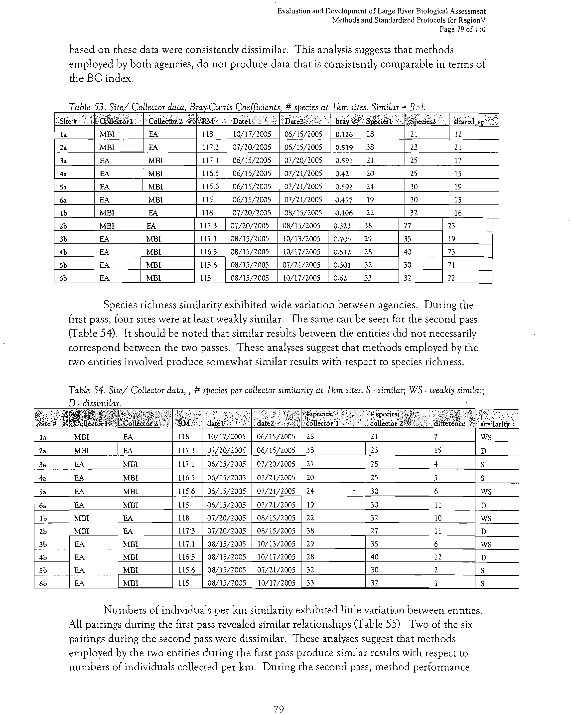
The results indeed showed a wide range of comparability from similar to dissimilar
results for individual sites and to a lesser extent for the overall average and range of results
for all sites combined with respect to each entity comparison. Raw catch differences
ranged from similar to dissimilar for species richness, density, biomass, and the MIwb. The
6
Evaluation and Development of Large River Biological Assessment Methods
Electrofishing Methods and Standardized Protocols for Region V
Page 7 of 110
Bray-Curtis coefficient showed mostly dissimilar results which may be an artifact of this
tool and the current thresholds for what constitutes "similar" results. This will require
further examination beyond the scope of this study. Nevertheless, it was the only
parameter that we felt was amenable to making comparisons among and between all
entities.
The results were deemed "comparable" with MBI in terms of average and site-
specific results for 3 of the 8 participating entities. For the remaining 5 entities, MBI
produced higher species richness and relative abundance, some by one order of magnitude
margins or greater. MBI electrofishing times exceeded most of the other entity times when
that data was available and seemed to be one of the factors associated with dissimilar
results in some, but not all of the comparisons.
We can make some preliminary conclusions at this time pending further analyses of
the results (see recommendations below), but it would appear that the factors involved in
the weakly similar and dissimilar results are electrofishing time (as a reflection of the
"thoroughness" of sampling), sampling procedures (e.g., sampling upstream vs.
downstream, daytime vs. nighttime, habitats sampled), equipment specifications and
settings (wattage, pulse settings, % of duty cycle), electrode configuration (anode array, use
of the boat hull as the cathode, etc.), site conditions (i.e., temporal water quality and flow
variations), and the general "intensity" of the sampling protocol and its execution. The
latter is not possible to conclusively confirm as we did not observe the operations of all of
the participating entities, but it may be inferred from electrofishing time results and the
descriptions and inherent nature of the cooperating entity sampling protocols. If these
conclusions hold pending more detailed investigation, gaining better comparability may be
a matter of standardizing the execution of the sampling protocols as opposed to making
wholesale changes in equipment. Standardizing results between different entities for
attaining consistent bioassessment outcomes would more likely be achieved by adherence
to a standardized sampling protocol. This would also be enhanced by conducting on-site
training as a mechanism for assuring consistency in the execution of the protocol. This
will be an important consideration for the upcoming U.S. EPA national large rivers survey
in 2008-9.
Cooperator Feedback
We afforded an opportunity for each participating entity to offer feedback and
make suggestions based on an earlier draft of this report. Concern was expressed by some
cooperators about the potential impact that this study might have on the status of their
current protocol and bioassessment program by extension. The bioassessment indices used
by each entity are to varying degrees
method and protocol dependent,
hence the impact of a
substantial change in methods is of concern. In at least one study area the potentially
confounding influence of temporal water quality conditions was raised as an undesirable
factor that might have compromised the comparability of the results. We agree that
minimizing external and potentially uncontrollable influences is a necessity in conducting
comparability studies. Ideally the comparisons would have been better controlled by
limiting the number f sampling locations, but that was impractical to accomplish for this
initial study.
7
Evaluation and Development of Large River Biological Assessment Methods
Electrofishing Methods and Standardized Protocols for Region V
Page 8 of 110
Perhaps the most significant concern was about the effect of the observed
differences on the resulting assessment of overall assemblage condition - do the observed
differences in raw catch statistics translate to a significant difference in the assignment of
condition for bioassessment purposes? We did not conduct sufficient analyses to answer
this question due to the limitations of the data analyses and the priority that was placed on
collecting the baseline comparison data. This is quite likely a non-linear phenomenon that
addresses not only the accuracy of a "pass/fail" presumption (at least one commenter
indicated the differences did indeed affect their assessment outcome), but also includes the
capacity to accurately measure along a continuous gradient of biological quality, i.e., the
U.S. EPA Biological Condition Gradient (U.S. EPA 2005; Davies and Jackson 2005). It
has been shown that the capacity to accurately measure across this gradient is a product of
the overall rigor of the bioassessment protocol that includes the aggregate effect of
methods, natural classification, reference condition, taxonomy, and other detail in the data
(Barbour and Yoder 2006). Two different protocols may well yield the same ability to
function within a general pass/fail dichotomy, yet be dissimilar in their capability to
accurately depict multiple categories of condition such as excellent, very good, good, fair,
poor, and very poor conditions and the margins between each. This capability is a
consistent prerequisite for supporting the development and application of tiered aquatic
life uses and a bioassessment framework that measures incremental change along a
biological condition gradient. Without first testing each resulting dataset across a gradient
of environmental quality, it will be difficult to determine how much the basic sampling
protocol and resulting dataset actually play in this issue. This could be examined at the
assessment outcome level of analysis that is recommended to follow this study.
Recommendations
In order to answer the important question about condition assessment
comparability, we recommend that further analyses be conducted, in particular calculating
Index of Biotic Integrity (IBI) values using the most applicable
calibrated
and
verified
IBI.
This would fulfill a key missing analysis by basing comparability on the
resulting
assessment of
condition,
rather than singularly focusing on baseline catch statistics. While this study
focused on making comparisons over a standardized sampling effort based on the same
unit of distance, comparisons of the net effect of each entity's protocol would also be of
value since this is a reality of the current state of electrofishing methods in Region V.
We also recommend that the results from each study area be discussed in greater
detail with each cooperator in an effort to more closely ascertain what factors the
differences are most attributable and what the impact of any implied changes in an existing
protocol might have. This will require detailed interactions with each entity that would be
enhanced by making observations of their sampling procedures in the field. We believe
this is one way of ensuring that the data collected by different entities is comparable for
bioassessment purposes across Region V. It would also have the benefit of being useful in
the development of applicability of QAPPs, training curricula, and methods for ensuring
comparable results and the resulting bioassessments that are produced.
8
Evaluation and Development of Large River Biological Assessment Methods
Electrofishing Methods and Standardized Protocols for Region V
Page 9 of 110
1. INTRODUCTION
1.1. Problem Definition and Background
Conducting biological assessments in large, non-wadeable rivers is widely regarded
as being more difficult and resource intensive than for smaller, wadeable streams, hence
the historical emphasis on this latter waterbody type by most states and EPA guidance for
aquatic bioassessments. The intent of this and its allied projects is to develop and evaluate
a process by which systematic and standardized methods for the biological assessment of
large, non-wadeable rivers can be made available to the states and EPA. This was and is an
important and requisite first step to attaining the goal of having fully developed and
calibrated biological assessment tools and biological criteria, which in turn supports
specific water quality management programs within the states and Region V. Of particular
interest here is the assessment of the effectiveness of NPDES permits on an individual and
collective basis by using the health of the biota as a keystone measure of response. This
will also have value to the national assessment of large rivers that is planned for 2008 and
2009 by U.S. EPA.
This project consisted of an assessment of fish assemblage electrofishing methods
used by selected Region V states, municipalities, research groups, private organizations,
ORSANCO, and U.S. EPA. The primary goal of this project was to evaluate a
methodology for determining the comparability of the different methods and protocols
and if the first order data produced by each is similar. This is a critical first step towards
the development and production of biological criteria and scientifically and statistically
valid assessments of the large river resources in the basins of the Ohio and Upper
Mississippi rivers within Region V. This project was designed to deliver a standardized
methodology that can be used by the EPA, the states, and other organizations in assessing
and managing their large river resources.
A systematic approach to assessing large, non-wadeable riverine resources is
presently an unmet need throughout much of the region (Yoder 2004). The knowledge
gained by this project is particularly useful in determining the ability of existing fish
assemblage assessment protocols to address water quality and aquatic resource management
concerns including status and trends, water quality standards (WQS), use attainability
analyses (UAAs), watershed planning, and NPDES permits. Collaborating organizations
included the states of Illinois, Indiana, Minnesota, Michigan, Wisconsin, and Ohio, all of
which contain large rivers that are tributaries to the Ohio and/or upper Mississippi Rivers.
Collaboration with U.S. EPA-ORD also took place as appropriate via a separate, but allied
project initiated by ORSANCO in 2004. Collaboration with the states and EPA occurred
with monitoring and studies already planned by each and as facilitated by the Region V
State Bioassessment Working Group. It should also be noted that this was intended to
serve as a possible first step towards the eventual determination of a standardized biological
assessment methodology and biological criteria, each of which are necessary to produce a
valid assessment of the large river resources of the region. We expect that the products of
this grant will be useful to the states for conducting long-term assessments of their riverine
resources.
9
Evaluation and Development of Large River Biological Assessment Methods
Electrofishing Methods and Standardized Protocols for Region V
Page 10 of 110
Large rivers are an important ecological resource and constitute a significant water
quality management challenge in the U.S. and elsewhere. They are the focus of numerous
environmental and natural resource management issues, which can be attributed in part to
their highly visible economic and natural resource values. In particular, numerous major
and significant NPDES permitted discharges occur in the large rivers of Region V. Despite
their importance and visibility, biological assessment methodologies are not as well
developed nor as widely employed in Region V as they are in smaller, wadeable streams,
and hence are only recently receiving emphasis by EPA and the states (Yoder 2004). This is
not to imply that the states are not interested or that some have not sampled large rivers,
when in fact most have some type of effort ongoing. However, sufficiently robust, refined,
and systematic large river fish assemblage assessment approaches and coverages that can
support biocriteria and TALUs have been developed and implemented by only two Region
V states and ORSANCO on a statewide or regional basis (Yoder and Smith 1999; Lyons et
al. 2001; Emery et al. 2003; Yoder et al. 2005). These were developed entirely within the
jurisdiction of each entity and are based on methods and equipment that may or may not
be transferable across the region. Ohio EPA developed standardized methods and adopted
numeric biocriteria based on calibrated multimetric indices (i.e., fish IBI) and adopted
numeric and TALU-based biocriteria in their WQS. Routine assessments of large river fish
assemblages have been conducted for more than 25 years (Ohio EPA 1987; Yoder and
Smith 1999; Yoder et al. 2005) and are accompanied by similarly developed
macroinvertebrate assessments. ORSANCO developed a fish assemblage method and
calibrated index for the Ohio River (ORFIn; Emery et al. 2003) for routine application
within their monitoring program and eventual adoption of biocriteria. Wisconsin DNR
developed a fish assemblage method and index (Lyons et al. 2001) that supports a
consistent statewide assessment of their large rivers. All three efforts are conceptually
similar, but exhibit differences in equipment and methods. Indiana DEM has developed a
working IBI for the Wabash River (Simon and Stahl 1998). The remaining Region V
states (Illinois, Michigan, and Minnesota) also sample large rivers, but not as extensively,
nor have they developed calibrated indices or numeric biocriteria. More importantly, each
state employs different equipment and methods, some of which are markedly different
from the other states and ORSANCO.
If the goal of having comparable assessments for the large rivers of Region V is to
be reasonably achieved, methodological issues need to be assessed. While there are
conceptual similarities in the different approaches presently employed by each state (e.g.,
all use boat-mounted electrofishing, all use it to generate assemblage level data in support
of bioassessment), there are important differences in the configuration and application of
the equipment, differences in the manufacture and design of the equipment, differences in
site sampling protocols, and differences in the execution of the sampling. The cumulative
result of these differences leaves important questions about the comparability of the data
and the resulting biological assessments unanswered. Besides the in-common issues of the
adequacy and comprehensiveness of individual approaches, the comparability of the
assessments produced by different protocols also needs to be established. For example, the
methods used by ORSANCO and the Region V states are generally similar, yet exhibit
explicit differences that potentially could produce different assessments of fish assemblage
10
Evaluation and Development of Large River Biological Assessment Methods
Elecrrofishing Methods and Standardized Protocols for Region V
Page 11 of 110
condition. Night electrofishing is one such variation in these methods that may affect
assessment results in the lower sections of the large river tributaries to the Ohio and Upper
Mississippi Rivers. Sanders (1991) discovered the advantages of night electrofishing in the
Ohio River while initially using a daytime methodology, an approach that ORSANCO
eventually adopted (Emery et al. 2003). It is therefore possible that the application of this
method may have merit over daytime electrofishing in the lower sections of the large river
tributaries to the Ohio and Upper Mississippi Rivers. Another variation is with sampling
distance covered at a site. Ohio EPA and ORSANCO sample fixed distances of 0.5 km,
which was developed based on extensive methods testing first accomplished by Gammon
(1976), which they independently retested (Yoder and Smith 1999; Emery et al. 2003).
Wisconsin uses a fixed distance of 1 mile, which is based on initial methods testing as well
(Lyons et al. 2001). This protocol is followed by Minnesota DNR and Michigan DNR and
IFR. EPA's EMAP program and some states employ a river width formula for determining
the dimensions of a sampling site. Some states sample both banks and the mid-channel
whereas others sample the "best habitat" available. Some states sample river sites in both
an upstream and downstream direction. Differences also exist in electrofishing gear
specifications, boat platforms, and electrode configurations. Finally, the execution of the
methodology at a site may also comprise a major factor in any observed variations between
protocols. This factor includes how deliberately and intensively a site is sampled. All of
these were examined and tested as much as was practicable in order to determine if
methodological differences alone could produce differences in the baseline data upon
which assignments of quality and condition (status) are ultimately based, thus making
comparability across the region more challenging.
It should also be noted here that assemblage level data is also used to characterize
and quantify reference condition, which plays a critical role in how the various assessment
tools are developed and calibrated in the process of establishing numeric biological criteria.
Evaluating the comparability of individual organization practices is very important in
determining the utility of bioassessments as a major program support tool. Large rivers
also present challenges in terms of shared and multiple jurisdictions. Therefore, a
regionally consistent approach to biological assessment and reference condition would
constitute a major advancement in the management of large rivers.
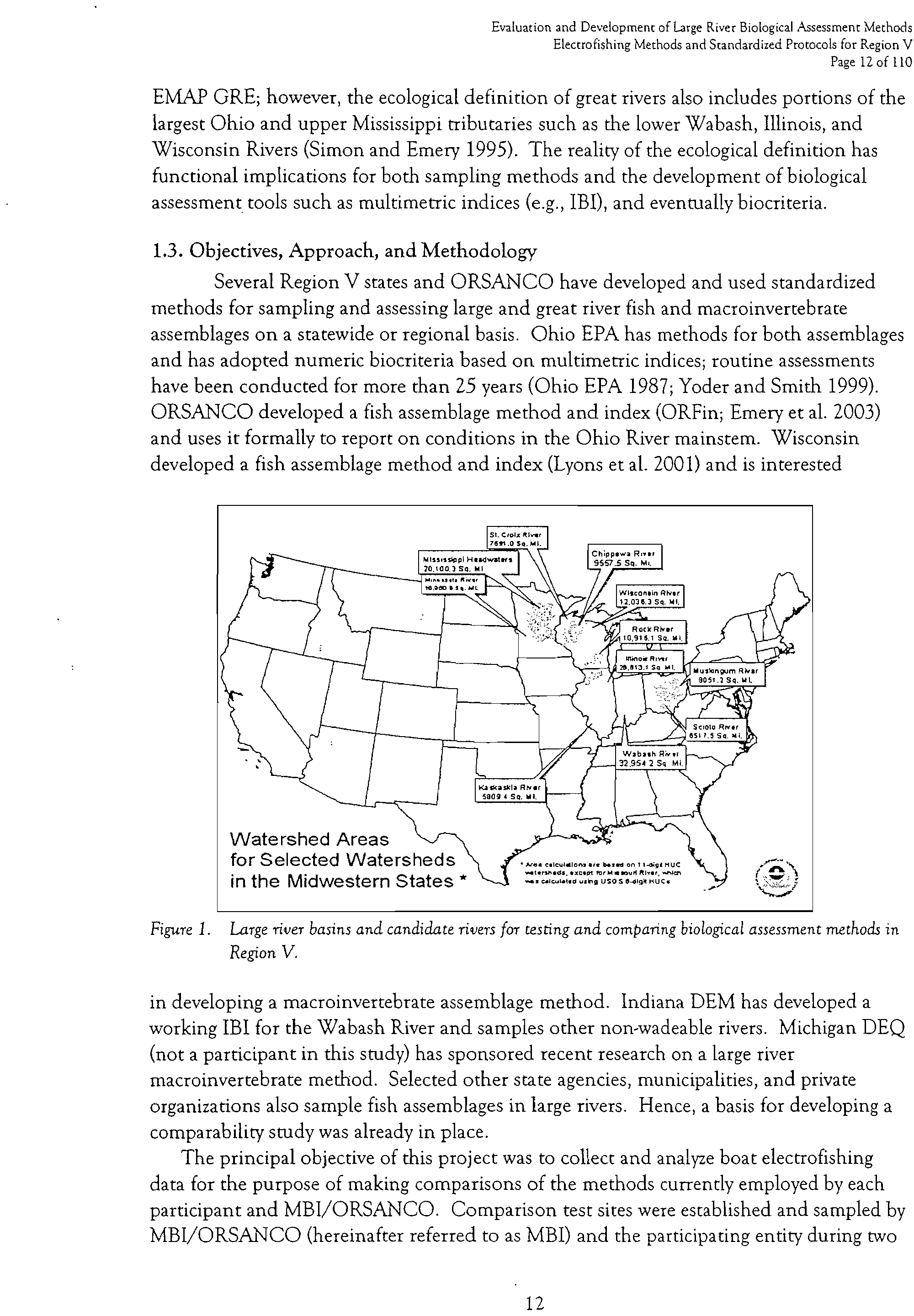
1.2. Geographic Area of Coverage
The geographic area of coverage of this study primarily included the large, non-
wadeable rivers that are tributary to the Upper Mississippi River (above the confluence
with the Ohio River) and the Ohio River that occur within Region V states (Figure 1).
One Great Lakes tributary and two entities were also included in the study in recognition
of this drainage within Region V. For the purposes of this project, large rivers are defined
as the primary tributaries of the Ohio and upper Mississippi Rivers and the Great Lakes,
and subsequent tributaries that drain land areas >500-1000 square miles. Non-wadeable
rivers that require boat electrofishing to secure an adequate assemblage assessment can
include drainage areas <500 square miles, but none were included in this study. An
interest of this and our allied river studies is to address the transition between great and
large rivers.. The Ohio and Mississippi are considered to be great rivers for the purposes of
1 1
St. <lo-lx /flyer
7601.0 SQ.
hi
I.
Allssess1901,11554.'"S
?
Chippewa River
20.100.3 Sq. MI
95575 Sq. 7711.
aill lira
?
WIscono,t ;Nor
lir?
12,035.3 Sq. MI.
R.1787.57
l0.916.1
AI
ScL
?
MI.?
liri
11104
17.55.7 ft vt
O
P '
25 5 31 SQ
Q. MUSIonpUrn RMar
0051.7 SQ. MI.
i'rilk(
‘?
"f
11.
?
CS MO R a
I
5517 5 SQ AI
11 il
liS
r al irl
1
ia
I
S k a Mr k
la a •1
0r
7
dp
•
I
Wabas
Sal' :
*AP
N
.
5009 4 Sq. MI.?
cue
• Nen. cal.1.11era •re 15.Q. en /1-aint.
....t•ran•..•QCOrn tar 1.1 • aw it lye
q
r,
I
...s Wunatetl using. LIS° S 64101 HU< Q.
....cr.
■
Watershed Areas
for Selected Watersheds
in the Midwestern States *
Evaluation and Development of Large River Biological Assessment Methods
Electrofishing Methods and Standardized Protocols for Region V
Page 12 of 110
EMAP GRE;
however, the ecological definition of great rivers also includes portions of the
largest Ohio and upper Mississippi tributaries such as the lower Wabash, Illinois, and
Wisconsin Rivers (Simon and Emery 1995). The reality of the ecological definition has
functional implications for both sampling methods and the development of biological
assessment tools such as multimetric indices (e.g., IBI), and eventually biocriteria.
1.3.
Objectives, Approach, and Methodology
Several Region V states and ORSANCO have developed and used standardized
methods for sampling and assessing large and great river fish and macroinvertebrate
assemblages on a statewide or regional basis. Ohio EPA has methods for both assemblages
and has adopted numeric biocriteria based on multimetric indices; routine assessments
have been conducted for more than 25 years (Ohio EPA
1987;
Yoder and Smith 1999).
ORSANCO developed a fish assemblage method and index (ORFin; Emery et al. 2003)
and uses it formally to report on conditions in the Ohio River mainstem. Wisconsin
developed a fish assemblage method and index (Lyons et al. 2001) and is interested
Figure
1. Large
river basins
and
candidate
rivers for testing and comparing biological
assessment methods
in
Region V.
in developing a macroinvertebrate assemblage method. Indiana DEM has developed a
working IBI for the Wabash River and samples other non-wadeable rivers. Michigan DEQ
(not a participant in this study) has sponsored recent research on a large river
macroinvertebrate method. Selected other state agencies, municipalities, and private
organizations also sample fish assemblages in large rivers. Hence, a basis for developing a
comparability study was already in place.
The principal objective of this project was to collect and analyze boat electrofishing
data for the purpose of making comparisons of the methods currently employed by each
participant and MBI/ORSANCO. Comparison test sites were established and sampled by
MBI/ORSANCO (hereinafter referred to as MBI) and the participating entity during two
12
Evaluation and Development of Large River Biological Assessment Methods
Electrofishing Methods and Standardized Protocols for Region V
Page 13 of 110
distinct periods within a summer-fall seasonal index period in 2004 and 2005. These sites
were established in various rivers in accordance with the detailed work plan and as
opportunities arose via allied projects and where other sampling was already planned by
the participating entities. What approximates "split samples" were obtained by sampling
each site using the ORSANCO nighttime method (Emery et al. 2003) and/or MBI daytime
method (Ohio EPA 1989; Yoder and Smith 1999) as the basis for comparison with the
participating entities. The decision about which of these two methods to use was based on
a site-specific judgment by the MBI crew leader, but was largely determined by where
mainstem rivers functionally transitioned from a large river to a wider and deeper great
river. At sites located at this transition both night and day methods were employed. Data
from two previous years was included for two cooperators in order to enhance the data
analyses.
In each comparison, sites were subdivided as needed to accomplish the protocols of
each participating organization. This yielded a side-by-side comparison of equivalent effort
based on cumulative sampling distance, which provided the weighted comparisons needed
to evaluate the basic data attributes and characteristics produced by each of the
methodologies. A minimum two-week period was used to separate sampling by MBI and
the participating entity for data collected in the same year. Of critical interest was
determining the minimum sampling effort needed to produce a reliable assessment of
biological quality and condition, which is an important prerequisite to producing
assessments at the regional and river reach scales. We spent a minimum of two weeks
sampling in each of the comparison study areas, based on detailed sampling plans
developed as part of the Quality Assurance Program Plan (QAPP). There were three
principal areas of testing and comparison:
1)
Equipment and design specifications - differences in electrofishing units (power,
output, duty cycle, efficiency), electrode configurations, boat size, etc.
2)
Protocols - differences in site configuration (best shoreline, both shorelines,
runs/riffles or pools, fixed distance vs. variable distance), CPUE basis (time or
distance), day vs. night, river flow or turbidity restrictions, net mesh size, number of
netters, single or multiple passes, taxonomic procedures, data recording and
custody, etc.
3)
Execution - "thoroughness" of the sampling, intensity of sampling within a site,
attention to detail, crew leader and crew member qualifications, skill and
knowledge, quality of workmanship, QA/QC adherence and documentation, etc.
This allowed us to evaluate potential differences yielded by key methodological and
technological issues and then determine if existing state methods are both adequate and
comparable, or if a different or modified set of methods should be adopted uniformly
across the region. Given the more advanced and broader application of fish assemblage
methods in the large rivers of Region V, we focused the study on this assemblage group.
13
Evaluation and Development of Large River Biological Assessment Methods
Electrofishing Methods and Standardized Protocols for Region V
Page 14 of 110
2.0. MATERIALS AND METHODS
2.1.
STUDY AREA/SITE DESCRIPTIONS
2.1.1. St. Croix River
The St. Croix River is a sixth order tributary to the upper Mississippi River that
originates at St. Croix Lake near Solon Springs, Wisconsin. The St. Croix River lies within
the Superior Upland and Central Lowland physiographic provinces. It is approximately
170 mi (276 km) long with a mean discharge of 131 m
3/s. Approximately 80% (129 miles)
of the St. Croix River forms part of the boundary between Wisconsin and Minnesota. The
upper 20% of the river is entirely within Wisconsin. The watershed covers approximately
20,098
km'
(7,760 mil) and extends from near Mille Lacs Lake in Minnesota on the west
to near Cable, Wisconsin, on the east. Approximately 46% of the watershed is located in
Minnesota. Originating in Upper St. Croix Lake near Solon Springs, Wisconsin, at an
elevation of 337 m(1,105 ft); it flows southwest to its confluence with the Mississippi River
at Prescott, Wisconsin (elevation 206 m, 675 ft) (Young and Hindall 1973). The
Namekagon River is a 5th order stream that drains northwestern Wisconsin and joins the
St. Croix above Danbury, Wisconsin. The St. Croix River is a National Wild and Scenic
Riverway and is considered one of the best recreational rivers in the Midwest. The river
exhibits moderate sinuosity and winds through primarily forested regions of Wisconsin
and Minnesota in a series of rapids and pools. The riverbed is primarily tillage with coarse
substrates throughout (DeLong 2005).
Comparisons were made on the St. Croix River between three agencies at a total of
ten sites between river miles 28 and 92 during the 2004 sampling season (index period)
(Figure 2). The participating entities included the Minnesota Pollution Control Agency
(MPCA) and the Minnesota Department of Natural Resources (MNDNR). Throughout the
index period, all three agencies executed their respective sampling protocols once (single
pass) at each site.
2.1.2. Wabash River
The Lower Wabash River is a seventh order tributary to the Ohio River and
incorporates the drainage basin between Honey Creek in Vigo County and the mouth of
the Wabash River at the Ohio River in Posey County. The river is approximately 475 mi
(765 km) long with a mean discharge of 1001 m
3
/s. The basin has an area of 1,339 mi.'
(Hoggatt 1975) and includes most of Sullivan and Posey Counties, plus parts of Vigo,
Greene, Knox, Gibson, and Vanderburgh Counties in southwestern Indiana. The major
cities and towns in the basin are Vincennes, Sullivan, and Princeton. The Lower Wabash
River valley is a broad, flat glacial drainage channel that includes winding channels, a wide
flood plain, and adjacent terrace levels. The valley floor ranges from 3 to 10 mi in width.
Local relief on the valley floor is typically less than 50 ft except for isolated hills (Fidlar
1948). Undulating, rolling plains with a thin cover of till, loess, and silt characterize the
area east of the Wabash terraces. Local relief is greater in the uplands of southern Posey
14
Evaluation and Development of Large River Biological Assessment Methods
Elecrrofishing Methods and Standardized Protocols for Region V
Page 15 of 110
County beyond the maximum extent of glaciation. Broad, flat lake plains that form present
day bottomlands east of the terraces were created during Wisconsinan time when tributary
valleys became ponded by the rapid aggradation of the valley floor (Fidlar, 1948, p. 102). In
the surrounding uplands, bedrock terraces were eroded on resistant limestone and shale.
Comparisons were made on the Wabash River with one entity at a total of seven
sites between river miles 23 and 257 during the 2004 sampling season (Figure 3). The
Indiana Department of Environmental Management (IDEM) executed their sampling
protocols once (single pass) at each site.
2.1.3. Wisconsin River
The Wisconsin River is an eighth order tributary of the Mississippi River,
approximately 430 mi (692 km) long, in the state of Wisconsin and drains an area of
31,080 km''. It originates in the forests of the Lake District of northern Wisconsin, in Lac
Vieux Desert near the border of the upper peninsula of Michigan. It flows southward
across the glacial plain of central Wisconsin, passing Wausau and Stevens Point. In
southern Wisconsin it encounters the terminal moraine formed during the last ice age,
where it forms the Dells of the Wisconsin River. North of Madison, it turns to the west,
flowing across the hills of southwest Wisconsin and joins the Mississippi approximately 10
mi (16 km) south of Prairie du Chien. It is navigable up to the town of Portage, 200 mi
(320 km) from its mouth, where it is separated from the Fox River by only 2 mi (3.2 km),
furnishing an important early route between Lake Michigan and the Mississippi for Native
Americans and early French explorers. The Wisconsin is impounded in 26 places for
hydroelectric power. The lower Wisconsin River is a shallow, sandy river of braided
channels among numerous vegetated islands. Turbulent currents create and obliterate
sandbars and bank holes with unpredictable frequency. Near Muscoda (RK 71.5), the
average discharge is 247 m
3
/s (Holmstrom et al. 1996). As the Wisconsin River passes
under a railroad bridge at RK 2.6, it becomes nearly indistinguishable from the side
channels and backwaters in Navigation Pool 10 of the upper Mississippi River.
Methodological comparisons were made on the Wisconsin River at a total of nine
sites between river miles 4 and 90 sampled by the Wisconsin Department of Natural
Resources (WDNR) during the 2005 sampling season (Figure 4) once (single pass) at each
site.
2.1.4. Kankakee River
The Kankakee River basin, located in northwestern Indiana, is the sixth largest
(2,989 mil) of the 12 water-management basins in the State. The basin includes most of
Newton, Jasper and Starke Counties and one-half to two-thirds of Lake, Porter, LaPorte, St.
Joseph, Marshall and Benton Counties. Most of the towns in the basin are farming
communities; the largest cities are LaPorte, Plymouth, Knox, and Rensselaer. It
encompasses approximately 3,000 square miles of river basin which includes at least
thirteen northwestern Indiana Counties. The topography of the watershed is flat to
15
Evaluation and Development of Large River Biological Assessment Methods
Electrofishing Methods and Standardized Protocols for Region V
Page 16 of 110
moderately rolling, expressing the effects of extensive glaciation. Sand and gravel river
bottom and scoured bedrock are indicators of glacial activity.
Land use in the river basin is predominantly agricultural, with over 75% of the
land used for cropland, pastureland, or forest land. Extensive corn, soybean, wheat, and
hay fields surround the Kankakee River. The Kankakee River drains 5,165 mi2 in
northeastern Illinois and northwestern Indiana (State of Indiana and others, 1976, p. III-
1). Within Indiana, the Kankakee River basin has an area of 2,989 mi2 (Hoggatt, 1975).
The Kankakee River begins in northwestern St. Joseph County and flows southwest for
about 80 mi before reaching Illinois. Before development of the area, the Kankakee River
was a large, meandering river surrounded by marshes. Now the river in Indiana is ditched,
has a gradient of about 1 ft/mi, and has been shortened to about one-third of its natural
stream length (State of Indiana and others, 1976, p. 111-24). The Kankakee River in Illinois
remains a naturally meandering stream. Principal tributaries are the Iroquois River,
Singleton Ditch, and the Yellow River with the Iroquois being the largest. The Kankakee
River in Illinois drains 2169 square miles and travels a distance of 62 miles from the state
line generally west to merge with the Des Plaines River and form the Illinois River. Almost
the entire Kankakee River basin in Illinois falls within the Kankakee Plain
physiogeographic subdivision. Most of the riverbed in Illinois is on or near bedrock.
Comparisons were made on the Kankakee River with the Indiana Department of
Environmental Management at a total of six sites between river miles 67 and 111 during
the 2004 sampling season (index period) once (single pass) at each site (Figure 5).
Comparisons were also made on the Kankakee River with the Illinois Department of
Natural Resources (IDNR) at a total of 13 sites between the Illinois/Indiana state line and
the Des Plaines River during the 2005 sampling season (index period) (Figure 6) once
(single pass) at each site.
2.1.5.
St. Joseph River (Lake Michigan tributary)
Although it is known locally as "the St. Joe River", it is associated with Lake
Michigan here because of the close proximity (less than 5 miles) of its headwaters to the
headwaters of the Saint Joseph River of the Maumee River watershed. The St. Joseph River
of Lake Michigan rises near Baw Beese Lake in Hillsdale County in southern Michigan.
While its course is generally westward to Lake Michigan, it is not direct.
From its headwaters, the St. Joseph flows northwest to southeastern Calhoun
County, passing the city of Hillsdale. It then turns directly southwest passing near the
Kalamazoo-Portage metropolitan area, eventually arriving at Three Rivers, so named for the
confluence in this vicinity of the Portage River from the north, and the Prairie River from
the southwest. Continuing southwest, it crosses the Indiana border and heads west
through the metropolitan areas of Elkhart - Goshen and South Bend, (named for the
river's abrupt turn north). Once back in Michigan the St. Joseph meanders roughly
northwest through the town of Niles, past the town of Berrien Springs and on to the
metropolitan area of St. Joe - Benton Harbor where it empties into Lake Michigan.
Approximately one mile from the mouth of the St. Joseph, it receives the Paw Paw River
from the north.
16
Evaluation and Development of Large River Biological Assessment Methods
Electrofishing Methods and Standardized Protocols for Region V
Page 17 of 110
The St. Joseph River watershed drains 4685 square miles in 15 counties, 8 in
Michigan and 7 in Indiana. Over 70 percent of the riparian habitat is agricultural / urban
and the rest (25-30 percent) is forested. Historically it furnished two important portages
that allowed for continuous river travel in the regional watersheds. The first, as has been
alluded to, was in the headwaters where portage could be made to the St. Joe of the
Maumee River which empties into Lake Erie. The second was in South Bend where a short
portage was all that was necessary to put in on the Kankakee River which flows into the
Illinois River, a tributary of the Mississippi River. In modern times, the damming of the St.
Joe restricts river traffic to the pools they form. From source to mouth there are 18 dams
on the mainstem, 14 in Michigan and 4 in Indiana.
Comparisons were made on the St. Joseph River during the 2005 sampling season
with the Michigan Institute for Fisheries Research (MIFR) (using methods described in
Lyons 2001) and the City of Elkhart Office of Public Works (EPW) (using standardized
IDEM protocols). MIFR and MBI executed their respective sampling protocols once
(single pass) at four sites, each 1 mile in length in Michigan (Figure 7). EPW sampled 15
sites of 500m each in Indiana (Figure 8).
2.1.6. Chicago Area Water System (CAWS)
The Chicago Area Water System (CAWS) comprises both natural and man-made
waterways, and it could be argued that the natural waterways are, in fact, only so in origin.
They lie within the Central Lowlands physiographic province which is divided into two
physiogeographic sections: the Great Lake Section and the Till Plains Section (Fenneman
1938). Leighton and others (1948) divided the Illinois part of these sections into two
subsections each. In the Illinois, the Great Lake Section was divided into the Chicago Lake
Plain and the Wheaton Morainal Plain. Most of the sampled waterways lie within the
Chicago Lake Plain subsection. Only the Sanitary - Ship Canal below its confluence with
the Des Plaines River and the Cal - Sag Channel below Worth, Illinois flow into the
Wheaton Morainal Plain. The Chicago Lake Plain consists of poorly drained lake clay and
silt and lake sand and gravel. Clayey till of the Wedron Formation also is present and is
deposited as moraines. The Wheaton Morainal Plain is predominately clayey till, sandy
loamy till, and sand and gravel. Limestone and dolomite bedrock underlies both of these
subsections. A large portion of the Sanitary - Ship Canal and the lower Cal - Sag Channel
were carved from this bedrock.
The topography of the land in the study area is relatively flat. It generally does not
vary more than 50 feet. This precipitates serious waste management problems for urban
areas. In 1822 Canal legislation was passed and the Illinois and Michigan Canal was
opened for river traffic in 1848. Up to the 1860's the city of Chicago had dumped its waste
into the Chicago River and ultimately into Lake Michigan, but in 1865 obtained
permission to pump sewage from the Chicago River into the Illinois & Michigan Canal. By
1881 the canal had become a health hazard. In 1889 the Chicago Sanitary District was
formed to build the Chicago Sanitary and Ship canal, the main channel of which was
completed in 1900. The Sanitary and Ship Canal extended from the Des Plaines River to
the Chicago River's south branch, causing a reversal of flow in the Chicago River, and
17
Evaluation and Development of Large River Biological Assessment Methods
Electrofishing Methods and Standardized Protocols for Region V
Page 18 of 110
diverting lake water into the Mississippi River system. Later, an additional North Shore
Channel was constructed from the north branch of the Chicago River to Lake Michigan.
Prior to 1900, the City of Chicago discharged sewage directly into Lake Michigan, the
Chicago River, and Calumet River. In 1922, the Sanitary District completed the Calumet-
Sag Channel extending the Sanitary and Ship Canal, and reversing the flow of the Calumet
and Little Calumet Rivers resulting in another diversion of lake water into Illinois. Today
sewage treatment plants treat most of the sewage before it reaches the waterways, but
combined sewer overflows remain a problem during flood events. The recently proposed
Tunnel and Reservoir Plan (TARP) is designed to ease that problem.
Comparisons were made the Aquatic Ecology Section of the Research and
Development Department of the Metropolitan Water Reclamation District of Greater
Chicago (MWRGC) on the North Shore Channel, the North Branch of the Chicago River,
the mouth of the Chicago River, the Sanitary Ship Canal, The Cal - Sag Channel and the
Calumet River at a total of 8 sites during the 2005 sampling season (index period) (Figure
9) once (single pass) at each site.
•
2.1.7. Scioto
River
The Scioto River is a sixth order tributary to the Ohio River, approximately 225 mi
(364 km) in length and drains an area of 16,882 km
2
. Mean discharge is 189 m 3/s. It is
contained entirely within Ohio, originating in the glacial till plains of the Central Lowland
physiographic province of Ohio in Auglaize County flows to its confluence with the Ohio
River at Portsmouth in Scioto County. It flows southeast across west-central Ohio,
becoming entrenched in the sloping landscape. From Chillicothe downstream the river
runs through the heavily forested Appalachian Plateaus physiographic province. Major
tributaries to the Scioto River include Big and Little Darby creeks; large portions of which
are designated as National Wild and Scenic River. The Scioto River is shallow and
generally sandy with some larger glacial till. The Scioto has not been heavily impounded
with the exception of two places in Franklin and Delaware counties respectively, creating
reservoirs for flood relief. Impacts from impoundments on the mainstem are low. However
middle portions near the confluence with the Olentangy River exhibit impacts from
increasing agriculture and urbanization (White et al. 2005).
Comparisons were made on the Scioto River between June and October during the
2005 sampling season at a total of six 500m sites with EA Engineering, Science and
Technology (on behalf of AEP (American Electric Power)) using methods similar to those
established by OEPA and employed by MBI. EA executed their protocol twice (two passes)
at each of six sites during June and August. MBI conducted two sampling runs at the exact
same geographic locations (Figure 10) during July and October.
18
tROtst.0.01E,
Tope
usn 5,0
•••
.Prairie Form ,
Adria. >a Satoc Croix
N,77".Cal
Oak Park
'Ile Grath
,Sanas toot
,Break Park 1
•Mori
F.'ioe?
r1-
;Ci-iifsburg
Reck Creek..
St.<1111e14.
a=S;eis'Io4c
Srandy
,
Flarranertq
_Cambridge
,Norh BriaZi
,Beltel•
una. ;B.ilsarii Lake
:•.
.,t7 •
?
xS+1.,CrvIzt Falls
.,•27f,:,;1-;;
L
"".r SChl`f
r31
W7110,
Willeraie
n4agolls
,L•ke Fla"
I
ftydsoa
a.,LF4
••keland
?
I
•
Data use subject to license.
02004 Detca-me. Topo LISPS 5.0,
www.delorme.com
MN (0.0' W)
IN MI MIN
•
MO?11111111
mi
0?
3?
6?
9 12 15
Data Zoom 8-4
Evaluation and Development of Large River Biological Assessment Methods
Electrofishing Methods and Standardized Protocols for Region V
Page 19 of 110
2.2.
SITE MAPS
2.2.1. St. Croix River (2004)
Fig. 2. St. Croix River
sites;
MBI (X), MNDNR
?
), MPCA (
?
); 2004.
19
Evaluation and Development of Large River Biological Assessment Methods
Elecrrofishing Methods and Standardized Protocols for Region
V
Page
20 of 110
Ri
ver (200
40#.6*;
?
Topa U SAT 4.0
Ag
u
e
.
Roy
'?
1St?
001'
?
..ill ^7
?
4?
..
:Wiamsport
,
?
,
Farmer Ciry44,,,
?
: ,.?
i
?
4'.C.: -
.:'
?i?
'44131-..,.)faholuet?
i
?
1,?
•?
Tr
n.
?.Colter?
\,...—
t
9■A_14
"'e4Qir.:7;u
'xbanally,—,=,;.,---.2?)4,-.4,--,-?
,Theratosnt: \
0?
Stif64,..
.
i"-
1?
s.„„
?
4.,,,,,,/ ‘c..tii..
-
-"fi
km
i
?
' iwasr,:iir
-13
?
..'4,
?
\
',.
-llontizeb
1?
i:
?
i?
1
?
:•!.
?
1"---
?
-,..:?
\
Telma?
IGO.trara 1 :
?
Le?
Me
'-`•c.
';
,Berueit i
?
:.•?
,.,
'...---•
?
1?
".
'Yllta Creme?
'''......—,.-",:iiarport,..
:..
,..B io;r1
:7674
•
?5
Newman
[loin!??
Paioill.C.1,-.....
Rangy
,..---
,
,fi.lert,–
la
..: Oakland
?
,C!AltrO,P,
?
-?
riditeSIC1Stie ?
..I'
?
,,../
.."'
?
e
'-'
;Sullivan
?
j
7.— ?
\
?
..,-*"."'"1.irerroactili
;
?
'
.10---.
.Cbarlestan
re-Ern-
1g
.......Br
e
.„,....„,,e;7".'
5hellmille
...
,,..„.....--,,
?
7 ;?
llartins vIlle
.lati
?
11?
-
V4 ga
?
.?,
.
?
..4Ca•O'aire;%31 I
Jelido
?
A. e ner,
z
?
.:,., .
e•
?
ree
p
F?
:
?
.Elleqtrille
?
'-,,-'
.
IV'
r2.-...,,,■
3
.?
.
.?
',Tut.
?
I
?
.Blooraiogrdu
'..-?
1 Sullivan?
It'orthinztort
;Ude:1m
?
Z '.4?
'?
L
?
e...,.._Illidattleld
;Celiton?
.11obluserr
4 iii1V:a■?
1?
/?
,
,
.1.
-t
?
'lets R.:.rt.
„Saukville, .:?
'?
.Bici:.a.ell
‘,.,
?
,
?
'0
?
::::liaritiaMiiler,
Brirliepert •?
1
?
,54,.,
?
'
).(itcl.eli ...;
f1...
.....;t
?
:
hn
is '?
orients
..: f ■-rnen Lick ?
Pa°li
ti
?
.•
?
:?
.:
?
.:.•k r,i.?
,vcr
';Yeterlliurg
Hardiailu
:?
cant Carmel•
?
F
__FalrfirId '?..,,Able.a
;Jasper
!'(
\
1
,,
'
Princeton
?
0 klaall
'cir •
, _ .?
'?
:..Eaglish
jiunria g1orf
?
.'
teratmech
1?
•
:
?
Frriirialul .
•...
.
.1.1cLeansbera?
C?
mi
Ohi(„f
A.
I
Chandler
?
Baconvil(e"
,..,•,•irt
Beaton
gt*a,), NI,-?
mosville?
It
■Zde7,1112e
—
skaL Vern
?
04...,u,s,
t
.,....
.•-c-?
it
JelvesiaTi Ciry ',
?
'Monde
?
.?
I
''
?
./.'
?
A,,,. ''/
?
..Ct;?
---?
A-?
• nsbiii•o,?
,...'
2rPr
?
'
?
' '
..-yc
ia,inilit11
—?
.Shi}:neetoo, n
1.i■lorganfleldP
i?
.?
'
Jrorrissine
....?
'..
i
Sna
?
•
rtis
?
'
1
?
,
Data use subject
to license.
S 2004
oeLorrne. Tops
?
U
A<!) 5.0.
111 MO
?
MIN?
MO
IN?
MIII
?
•
?
mi
0?
6?
12?
18
?
24?
30?
36
WWW .delorme
corn?
F.% (00'
W)
?
Data Zoom 7.3
Fig. 3. Wabash
River
sites; MBI (X),
IDEM?
, ); 2004.
20
Evaluation and Development of Large River Biological Assessment Methods
Electrofishing Methods and Standardized Protocols for Region V
Page 21 of 110
2.2.3. Wisconsin River (2005)
Topo USA
?
5.0
.
'Mum?
,}CeezIal/?
liauSta .
,...
';-
„Cashion
?
Jlray
Pncarla?
A,
„CUOu Vallee
`', 3.. den Sudo.
talun Cesare
„,„,',..",,,WesIV.
?
„lilllabero?
•-•Wanruec
1-
WS.021111oati7.
...
' :
,Lafarie
?
Lii,alLe
•
?
,
?Viroqua
.,..
•
Summit?
"-lit:..i'4'-;
,..,,i,lela
Rock Spilup
,
Cirat Alelie
?
.1.
?
••.
•
A
`
Baraboo
Rea
"
41scenat
',
L
i
p".
...,:,_„1.,evurellle
•\ortfi Freres-
.".tuldlers Gr•nse
.?
..
2 „Ferrvrille?
\-.'
-;•
idAaRMiTti
?
Crater
0
310•Itt S itr 1 fa :?
,
G.Y,
Yin.?
.
,ta7
;Learlille
...
?
?
Seneca .
,
(
Seltutrat
?
.?
_ ,
?Plain
_...
Prairie
?Sauk
iu Sae
ein.,
j
•
?•
.:t2es.:rktUY -itkl,iliq!ttu..-19;15.,'727Wi'l
e
i
?
ACI
a
?
?
A,.-::......Ittua.R.c1::*e
"
?
...
Eastman
?
,?
•?
Steuben?
..
.
s....•
lezcanasle
escebet
Black tan
.Wa
r.
?
f-,,
e
t l.
r?
•
,
Ilighlaad
Barnewld
,Bluel/aeude
'd ,?
'''Clgigrilirek:„."-,,,,
',..
,,,,..TINIatrat llopc?
t""''""""?
''',..2,M,""i
?•C°ik......Diittigiffg';‘,.
'
:kach
.
Grere . ,
,Sricztr
Lluden
.:.
,
Bagle!?
.I..irenrman ',.
Blo?mingin
?
.,
?
,,...: ?
i
,Hollandale
...,9'
d
?
rAlineral 'Point
;Laacasler ?
•
?
t?
Reuel'
?
;
?
•
.
Glen Haren
carenberg?
3.
',. ,Bleucherthille
1
W
I
:-•21
u• •
?
aslant
-..
Casa.111.
;ti
rkButut
.?
-
VIcra
-"IDati.logtol
5%...11. c. Di
iblckepille?
..
Luxer,kurk
4?
?
.
Holy Cross?
;Slat rrl/I
,1
?
Sulaa Cliy
.?
....?
„Iileler
?
„Ile,,atou
?
,Shullsburg
''1..P,;C4.C.,?
South
Waeue
?
raaatena
'
?
V.
?
Hazel Criett
el3tlque
^?-'-
.^:-'' -.- - _?
•?
- - - - , - - - , - 7.-- .491.-Iti.r.11-th.r?
-....-faifois-•-•'-
.11-
,
veriville
?
''''?
'''' East Dubuque
?
Scales .Nlound
i
a
ILT-.12-,...,..,
?
,,..a..._„."
?
McCoun'ell
„;
Gefeaa
Data use subject to license
?
711.?
IN
?
MIN
?
NOM
?
MEI
ml
MI?
OM
?
MIN
0 2004 OeLorme. Tops USA
?5 0.?
0?
3?
6?
9?
12?
15?
18
iii,-.•ividelornle.com
Mll 0.0' W)
?
Data Zoom 8-3
Fig. 4. Wisconsin River
sites;
MBI (X), WDNR (
?
);
2005.
21
51141:16„A
r
?
Topo U SAM 5.0
Data use subject
to
license.
fg
, 2004 DeLorne..Topo USAt 5 0.
www.delorrne.com
III?
■
IN
MI
II
MI
II
MI
MI
mi
0
?
2 3 4 5 6 7 8 9
MN (0.0° W)
?
Data.Zoom 9-4
Evaluation and Development of Large River Biological Assessment Methods
Elecrrofishing Methods and Standardized Protocols for Region V
Page 22 of
110
2.2.4. Kankakee River (2004)
Fig. 5. Kankakee River
sites;
MBI (X), IDEM (
); 2004.
22
4
4.:4110.
Top°
USAZ)
5.0
mi
10
MN (0.0* VV)
"";tfiratt;r<ii...,
Morena.
liossenteoel
C.)
,Floe smear?
_Cleanest
lfakeoa
,Frak.fort,_„,
,Otsepia Beide
,Parkforest
• Riclava Pick
,Sts-ger
..Elsrooel
Pecroae
/
tl7lath:aa
'>Istoieno
nu; Perk
•
Mal Y'PF431:!•1.1.
,
Boalle?
•`,,
ye,
1,..Rvi.17
.Caiest Hill
Hetlids
!Ai
?ark
Buckle gilase
eases:dile
.Kesapien
S51.4a7"s:,
=III
0?
2?
4?
6?
8
Data
Zoom 9.2
Data use subject to license.
0 2004 Delorme. Topo USA0 5.0.
mvw.delorme.com
Evaluation and Development of Large River Biological Assessment Methods
Electrofishing Methods and Standardized Protocols for Region V
Page 23 of 110
2.2.5. Kankakee River (2005)
Fig. 6. Kankakee
River
sites;
MBI,
IDNR (X.);
2005.
23
Topo USAF
5.0
4.PLyilrovell
.Laccga
,GrasclJusction
_Bloomingdale
,Cnitics
Scrert
••.y.
!
Vy,
?tyylesbur;,..
A?
4
lamazoo
.0alauatt
jlareford
yortaget,
•
•;Lawirnet
?
Parr Fait
/
Suns,
,Decatur
.11arce/lus
W
ou
•
ers
..
_Centre-cam
lames
cCeacuerine
rate
Lisa - —?
•
St
Fm.
Ilarre
JAV141tt:
• akcy
:Wyatt
Waturusi
.NtUlersburg
.Tafelca
New:Paris
a Pat
?
ye"""--
,,,NI
&Bums
Syracuse
•
Cromwell
z?
,Albion,
2.2.6. St. Joseph River (2005)
Data use subject to license.
02004 DeLorme. Topo USA 5.0.
swror.detorme.com
1
C.
MN (0
W)
•
•
•
NI
EN
NI
I=
•III
ml
0 2 4 6 8 10 12 14
Data Zoom 8
-
8
Evaluation and Development of Large River Biological Assessment Methods
Electrofishing Methods and Standardized Protocols for Region V
Page 24 of 1.10
Fig. 7. St. Joseph
River I mile
sites;
MBI, MIFR (X);
2005.
24
Evaluation and Development of Large River Biological Assessment Methods
Electrofishing Methods and Standardized Protocols for Region V
Page 25 of 110
2.2.7.
St. Joseph River 500m Sites (2005)
pso
Topo U SAID 5,0
in
.
1
i
e?
1
?
c:—"
(
_.,---
c
,s.,_
.
i
..,?t
,
?.-->
--.
IA
',.../7-1,
-
:?ft
..,
1
'
alnes
‘:Wakar42
-
I
3• 1
w
.,
...
---:-
.A.
EEEit
:.=-4--.
?
=.: ---.
?
_-.-..:
—?
,
,n'cr,
Cr2
f
k
,
.-...
-
!...0
••
■V•
?
I
?
-,
2.,
L
1
?
,:i
.
.-■
??
S5
.
..
-79.1
(
•?J
,
1-kevine
41.81.5■1S
i
G orfetowz
11,1?
_,_-,_..
,
0a...v...-oe.
PS,S21-C
1110,13
.
?l.fl ,
_
,.....
si
ss;
!.-.3.t
:
.0
A.,-
',..
Duct/
71?1?
\
..
.....?
.,.
\■-;
G u liv I?
P;FI
I.
?
rt
•
!.■
ctzt.
,?
P,
,
Data use subject to license,
e 2004 DeLorrne. Topo USA
?
5.0.
mvw.delorme.corn
j (0.0'W)
NI?
MIN?
MIIII
MI?
Mil?
MN MI
0
?
1
?
2
?
3
?
4?
5
Data Zoom 10-0
Fig. 8.
St.
Joseph
River 500m
sites; MBI, EPW (X); 2005.
25
Evaluation and Development of Large River Biological Assessment Methods
Electrofishing Methods and Standardized Protocols for Region V
Page 26 of 110
2.2.8. Chicago Area Water System (2005)
b
g
bditrift?
Topo U SAO 5.0
–r
a
Er
Oaladie .?
Willossks
-.2.
,:d''
11
_,
...* '''Ae.,..?
„irospeelRe4,1•11,.?
.
'?
ArAagtall
:?
,
?
Rolling
Ireighas
,,
Stevie.,
?
?
'
?
t'
?\`
''1
?
Xeoiliseeth
.11
-,..?
.wil.,,,,,?
41!I I.V.54E:v.
...U.13";
...?
.0tesavie
,c.ir
\
'
l
?
*
Earns; rotates .?
.
:`?
Schauroburi
,
?
,DetTlaless
.,..,...i.—,'-aa......,
?
,,,,„.
?
34''',,./?
C
'F'
?
'.?
.12172,5C5!C:i.;..-
.':,;,!
''
?
.r.
..Milks
?
1,1311.45Cit.T..
li.
g 5
,
I
'..... —,
Elk Greve Villa;?
,..
..
.-,?
"ark Ridge .?
1111Cilitreqi
X
ELVN o HAR7 EXPY '?
.
7,
.,,-"
-- -77
.?'.
?,?
•,;? ,I` "?
,
I..
?
•
Roselle
?
?
Midi.
'
?
,
•..
—r.
?
4 ,...?'?
..a...
-
..,....,,,,
?
? ?7r.,..,..---1
.....
'?
sso
?
,:„,
1.
.
WrOod Dale
?
— : \--.•:•:—
?
Harwood
?
.
pl000llog?
le?
,
?
marine /
?.Schiller Rork?
•
,Fraltslin Park?
.
.
?
i.
,
?
?
.
•
-
Riser Groat'El...rood:Park.
?
Zi,
',.
?
.c
""fl S.*'?
lesidalo?ieigkis?
St:.
:
Illa Park
?
•
Eloshisrsz
fi
?
?
,Berkiley
giaeo:e Park
:?'.?
'
?
Ila?
•Rh
;ask
'i"
Park
."'?
?
8,
Naza.o..,,,n!
0',
,?
:: .:.1..i31::-.
.
..s.:
Gin Filly?
.1-?
.
Ilellorsosl?
,ForestPark
•Whelion
...
i?
/11-yer014•
•-st=?
wor,..:
NS estekever
. .?
?
Beearbitts
likes?
?
„BtroTo
I
C
O
.1
?
ix
:: i L3
Graag,Fark .?
,Riverxida?
,Cisero
?
..x
,,
:'Oak Brook
?
Besokllai
a
?
?
= ` . ,:rTst,,fr
.?,.
.
?
.1....Crails.`''"-1
,,,
......_ ... ..._ ,.
?
°:":-
?
.
6
2:?:'••
•?
• '''`'..".
?
,Hinsdale
:■.:?
-Westers4prings?
4
..'"
ci.,,,,a.. Hid.
,....,
an
,?
CB
„WoOdridgeustiee
:sO"''
.?
Brklgedele
"wills?
sprint:
\"
.
.1
?j
?
?
'
?
BarOsak?
'
lioloeloosa
jIrc4
:4
1
. '111111'?
..--;-Oak Lawn
?
s...,.........
BoUngtra
?
o
epoles Hills,
Worth
ens
.opok, Rork
r^S
?
,Paloelieliso.it.
„Rea
3117...az.sP. 152-2:
,Rotlalos
••■
rlavl Park?
R?
,Ril eniale
"NtitIllisfilit4"
Doke..
11
...
..a....?
. a ..?
,??
a9AChg
ell
an4...
..
Lockport?
..
Data use subject to license.
?
Ilit
?
■
■
NM
MI
NM
MI
MN
NE ml
To 2004 Delorme. Topo USA
?
5.0.
?
0?
1?
2?
3?
4?
5?
6?
7
www.delorme.com
?
LAN
air
NO?
Data Zoom 9-6
Fig. 9.
Chicago Area
Water
System
sites;
MBI, MWRGCA (X);
2005.
26
150:Pkitiit
Topo
USk
5.0
Data use subject to license.
2004 DeLorme. Topa t.ISA4
www.deforme.com
0
1.11
MI -
400 800 1200 1000 2000 2400 2800
MN (0.0' W)
Data
Zoom
13-5
Evaluation and Development of Large River Biological Assessment Methods
Elecrrofishing Methods and Standardized Protocols for Region V
Page 27 of 110
2.2.9. Scioto River (2005)
Fig. 10.
Scioto River
sites;
MBI, EA (X);
2005.
27
Evaluation and Development of Large River Biological Assessment Methods
Electrofishing Methods and Standardized Protocols for Region V
Page 28 of 110
2.3.
SAMPLING EQUIPMENT/ PROTOCOLS
2.3.1. Midwest Biodiversity Institute (MBI) and ORSANCO
Sampling
Procedure
The standard MBI and ORSANCO large river (non-wadeable) sampling protocols
include boat electrofishing and habitat evaluation at each site. The methods and
approaches described by Ohio EPA (1989) and Yoder and Smith (1999) for the collection
of daytime samples and Emery et al. (2003) for the collection of nighttime samples were
used to generate the baseline data that served as a comparison to the individual
cooperating entity methods. As such, the MBI and ORSANCO methods are the default
arbiter of comparability.
A boat-rigged, pulsed D.C. electrofishing apparatus was the single gear employed in
this study. This consisted of a 16' (daytime) or 19.5' (nighttime) aluminum boat
specifically constructed and modified for electrofishing. Electric current was converted,
controlled, and regulated by Smith-Root 5.0 GPP alternator-pulsator that produced up to
1000 volts DC at 10-20 amperes depending on relative conductivity and power output.
The latter was adjusted to the maximum range that could be produced given the relative
conductivity of the water. The pulse configuration consisted of a fast rise, slow decay wave
that can be adjusted to 30, 60, or 120 Hz (pulses per second). Generally, electrofishing was
conducted at 120 Hz, but other settings were used depending on which selection was
producing the optimum combination of voltage and amperage output and most effectively
stunning fish. This was determined on a trial and error basis at the beginning of each boat
electrofishing zone and the settings generally held for similar reaches of the same river. On
the 16' daytime boat, the electrode array consisted of four 8' long cathodes (negative
polarity; 1" diameter flexible stainless steel conduit) which were suspended from the bow
and 5 anodes (positive polarity; 3/8" by 4" in length woven stainless steel cable) suspended
from a retractable aluminum boom that extended 2.75 meters in front of the bow. These
could be added, detached, and replaced as conditions changed. The width of the array was
0.9 meters. Anodes and cathodes were replaced when they were lost, damaged, or became
worn. For the 18' nighttime boat, the boat hull, in combination with 32, 3/8" woven steel
cable strands bolted to angle iron welded to the bow, served as cathodes. The anodes
consisted of a pair of Smith-Root retractable fiberglass standard GPP booms each fitted
with removable Smith-Root LPA-6 low profile 3/8" woven steel cable dropper arrays.
Illumination for nighttime sampling was provided by 12 volt DC lights supplemented by
auxiliary headlamps worn by the sampling crew (which consists of a driver and 2 netters)
and hand held lamps of at least 1,000,000 candle power. •
The sampling procedure was to slowly and methodically maneuver the
electrofishing boat in a
down
-
current
direction along the shoreline of the bank with the "best
habitat" following the original design of Gammon (1973, 1976). This generally included
sampling along the outside bends of meandering rivers and/or the bank with deeper water
and the most diversity of cover types. It also included sampling deep run habitats which
are what might be regarded as mid-channel habitats. Sampling was performed by
maneuvering the boat in and around submerged cover to advantageously position the
28
Evaluation and Development of Large River Biological Assessment Methods
Electrofishing Methods and Standardized Protocols for Region V
Page 29 of 110
netter to pick up stunned and immobilized fish. At times this required frequent turning,
circling back upstream, backing in and out of cover, shifting between forward and reverse,
changing speed, etc. depending on current velocity and cover density and variability. The
driver's task was to maneuver the electrofishing boat in a manner that advantageously
positioned the netter(s) to pick up stunned and immobilized fish. The driver also
monitored and adjusted the 5.0 GPP pulsator to provide the maximum, yet safe
operational mode in terms of voltage range, pulse setting, and amperage. In areas with
extensive woody debris and submergent aquatic macrophytes, it was necessary to maneuver
the boat in and out of these "pockets" of habitat and wait for fish to appear within the
netter's field of view. In moderately swift to fast current the procedure was to electrofish
with or slightly ahead of the current through fast water sections and then return upstream
to more thoroughly sample eddies and side edges of the faster water. It was often necessary
to pass over these swift water areas 2-3 times to ensure adequate sampling.
Electrofishing efficiency was enhanced by keeping the boat and electric field
moving with or at a slightly faster rate than the prevailing current velocity. This allowed
the field to remain vertically extended as opposed to being collapsed against the bottom of
the boat by the resistance of the current. In addition, fish are generally oriented into the
current and must turn sideways or swim into the approaching electric field to escape. As
such they present an increased voltage gradient making the fish more susceptible to the
electric current. Sampling these areas in an upstream direction was avoided as this
collapses the electrical field upwards against the boat, which significantly diminishes the
effective volume of the field. Based on visual observations and our experience, fish can
avoid capture more easily when sampling against the current. Although sampling effort is
measured by distance, the time fished was an important indicator of adequate effort. Time
fished could legitimately vary over the same distance as dictated by cover and current
conditions and the number of fish encountered. In most cases; there was a minimum time
spent sampling each zone regardless of the difficulty or size of the catch. In our experience
this was generally in the range of 2000
.
2500 seconds of electrofishing time (time during
which current is actively applied to water) for 500 meters, but could range upwards to
3000-3500 seconds or more where there was extensive instream cover and slack flows.
Time was recorded in seconds on the 5.0 GPP control unit and recorded on each
electrofishing data sheet.
Safety features included easily accessible toggle switches on the pulsator unit and
next to the driver and a foot pedal switch operated by the primary netter. Netters wore
jacket style personal floatation devices and rubber gloves. Sampling was conducted
between June 16 and October 30. This represented the seasonal index period developed
for the Ohio River for assessing the overall fish assemblage in keeping with the goals and
objectives of the study. However, earlier cutoff dates were adhered to when established by
individual states.
Netters were required to wear polarized sunglasses during daylight to facilitate
seeing stunned fish in the water during each daytime boat electrofishing run (not required
for nighttime runs). Smith-Root heavy duty dip nets with 2.5m long fiberglass handles and
7.62mm Atlas mesh knotless netting were used to capture stunned fish as they were
attracted to the anode array and/or stunned. A concerted effort was made to capture every
29
Evaluation and Development of Large River Biological Assessment Methods
Electrofishing Methods and Standardized Protocols for Region V
Page 30 of 110
fish sighted by both the netters and driver. Since the ability of the netters to see stunned
and immobilized fish was partly dependent on water clarity, sampling was conducted only
during periods of "normal" water clarity and flows. Periods of abnormally high turbidity
and flows were avoided due to their negative influence on sampling efficiency. If high flow
conditions prevailed, sampling was postponed until flows and water clarity returned to
seasonal, low flow norms.
Field
Sample
Processing Procedures
Captured fish were immediately placed in an on-board live well for processing.
Water was replaced regularly in warm weather to maintain adequate dissolved oxygen levels
in the water, reduce waste by-products, and minimize mortality. Aeration was provided to
further minimize stress and mortality. Fish that were not retained for vouchers for
laboratory identification were released back into the water after they were identified to
species, examined for external anomalies, weighed, and measured for total length. Every
effort was made to minimize holding and handling times. Invasive alien species were kept
and appropriately disposed of out of the water as required by state collecting permits. The
majority of captured fish were identified to species in the field; however, small specimens
(mostly Cyprinidae) were preserved for later laboratory identification to ensure both
accurate identifications and enumeration.
Any uncertainty about the field identification of individual fish also required their
preservation for later laboratory identification, except for unusually large specimens that
were photographed. Fish were preserved for future identification in buffered 10%
formalin and labeled by date, river, collector(s) and geographic identifier (e.g., river mile,
site number). Identification was required to the species level at a minimum and to the sub-
specific level in certain instances if necessary. We followed the scientific naming
nomenclature in Nelson et al. (2006). A number of regional ichthyology keys were used
and included Page and Burr (1991), Trautman (1981), Lee et al. (1980), Etnier and Stames
(1993), and Tomelleri and Eberle (1990). Questions were pursued with the recognized
taxonomical expert in each state.
The sample from each site was processed by counting individuals and recording
weights and total lengths by species. Total lengths of each specimen were recorded to the
nearest 3 cm size class, with 0.1 cm to 3 cm representing size class 1, and so on. Fish
weighing less than 1000 grams were weighed to the nearest gram on a spring dial scale
(1000 x 2g) with those weighing more than 1000 grams weighed to the nearest 25 grams on
a 12 kg spring dial scale (12 kg x 50 g). Scales were properly zeroed prior to each individual
sampling run. Individuals of the same species within the same size class were weighed
together. If too many individuals of a given species were encountered to make individual
weighing and measuring practical, mass weights were taken via a systematic subsampling
process. Larval fish were excluded in the data, as these are not only difficult to identify,
but offer questionable information to an assemblage assessment (Angermier and Karr
1986).
The incidence of external anomalies was recorded following procedures outlined by
Ohio EPA (1989) and refinements made by Sanders et al. (1999). All external
abnormalities were recorded and included any type of deformity, lesions, tumor, parasite,
30
Evaluation and Development of Large River Biological Assessment Methods
Electrofishing Methods and Standardized Protocols for Region V
Page 31 of 110
or other body part anomaly. The frequency of DELT anomalies (deformities, eroded fins
and body parts, lesions, and tumors) is an essential indicator of stress caused by chronic
agents, intermittent stresses, and chemically contaminated sediments. The percent DELT
anomalies is a metric in most of the large river fish assemblage assessments that have been
developed across the U.S. Crew members were trained to recognize anomalies prior to
each field season.
Habitat
Evaluation
Prior to conducting electrofishing at each site, the field crew completed
ORSANCO's Habitat Data Collection Protocol (2003) as outlined in Appendix 2. This
procedure is a physical evaluation of the benthic macrohabitat features and immediate
riparian characteristics within the designated sampling area. This is a thorough yet rapid
evaluation technique employed by agencies for the purpose of developing expectation of
site specific performance. Habitat characteristics were recorded after the completion of
sampling at each site using a qualitative, observation based method (Rankin 1989, 1995)
under seasonal low flow conditions. Attributes of the Qualitative Habitat Evaluation
Index (QHEI) include substrate diversity and composition, degree of embeddedness, cover
types and amounts, flow velocity, channel morphology, riparian condition and
composition, and pool and run-riffle depths. The original QHEI (QHEI; Ohio EPA 1989;
Rankin 1989) was modified for application to non-wadeable rivers (Appendix 2) and was
completed by the crew leader at the completion of each electrofishing event. The QHEI is
a physical habitat index designed to provide an empirical, qualified evaluation of the lotic
macrohabitat characteristics that are important to fish assemblages. The QHEI was
developed within several constraints associated with the practicalities of conducting a large-
scale monitoring program, i.e., the need for a rapid assessment tool that yields meaningful
information and which takes advantage of the knowledge and insights of experienced field'
biologists who are conducting biological assessments. This index has been used widely
outside of Ohio and similar habitat evaluation techniques are in widespread existence
throughout the U.S. It incorporates the types and quality substrate, the types and amounts
of instream cover, several characteristics of channel morphology, riparian zone extent and
quality, bank stability and condition, and pool-run-riffle quality and characteristics. Slope
or gradient is also factored into the QHEI score. We followed the specific guidance and
scoring procedures outlined in Ohio EPA (1989) and Rankin (1989). A QHEI habitat
assessment form was completed by the crew leader for each zone over the standard 500
meters of sampling distance (see Appendix 2).
Local gradient was determined from USGS 7.5' topographic maps and water
clarity was measured with a secchi disk. Water quality included basic field parameters such
as temperature, dissolved oxygen, and conductivity. These were determined at each
sampling location with portable meters and at fewer locations using continuous
monitoring devices. The habitat evaluation methods provide an ancillary benefit to the
sampling crew by revealing various features within the sampling reach that must be
included, but may not be considered upon initial visual inspection. These data help
facilitate a thorough execution of the electrofishing protocol.
31
Evaluation and Development of Large River Biological Assessment Methods
Electrofishing Methods and Standardized Protocols for Region V
Page 32 of 110
Field Data
Recording
Field data and observations were recorded on water resistant data sheets. Fish
assemblage data including species, size class, numbers and weights by species and size class,
external anomalies, chemical/physical data, site name and numeration, sampling crew
membership, time of day, time sampled, distance sampled, and electrofishing unit settings
and electrode configurations will be recorded on the fish sampling data sheet (Appendix 2).
Data sheets are retained by ORSANCO and MBI. Voucher specimens collected by
ORSANCO crews were deposited at ORSANCO for a period of one year then moved to
the Center for Ohio River Research and Education at the Thomas More College Ohio
River Biological Field Station for storage/ archiving. Samples collected by MBI were
permanently deposited at the Ohio State University Museum of Biodiversity. As such they
provide a permanent record. The vouchers served to validate new species distribution
records and for verification of questionable field identifications. Each set of vouchers were
labeled with the same location data recorded on the field sheet and they are also denoted
on the field sheet. All data were entered into an electronic data format maintained and
supported by ORSANCO. At this time we are using a Microsoft Access database, which is
translatable to spreadsheet formats such as Microsoft Excel.
2.3.2. Minnesota
DNR
Sampling Procedure
The Minnesota Department of Natural Resources (MNDNR) large river (non-
wadeable) sampling protocol includes both electrofishing and habitat evaluation at each
site. A modification of the method and approach described by Lyons et al. (2001) for the
collection of fish by boat electrofishing was used at each site to generate the data that
would be incorporated into the state's monitoring initiative. The principal modifications
include a smaller dip net mesh size and two netters.
Fish were collected using a boat-mounted, VVP-15 Coeffelt pulsed-DC
electrofishing unit. A 17-foot long aluminum boat with 6, 5/16-inch stainless steel cables
serving as the cathode was the primary electrofishing platform. The anode was a single 4m
boom with a "Wisconsin ring", from which 16 cylindrical, 17mm diameter stainless steel
droppers were suspended (Lyons et al. 2001). About 125mm of each dropper was in
contact with the water. This cathode array is not commercially available. Electricity was
provided by a gasoline-powered AC generator rated at 5,000W. The sampling crew
maintained 300 volts at 5-lamps, 30% duty cycle, and 60% frequency through the control
box. Electrofishing time was recorded in seconds on the control box and recorded on the
data sheets.
During sampling, two crewmembers used 1/8" mesh dip nets and attempted to
capture all of the stunned fish. Captured fish were identified to species, counted, and
weighed in the aggregate by species. Most specimens were released after processing.
At each sampling site 1,600m (1 mile) of channel border habitat was sampled on one bank
with the first 500m processed separately for the purpose of this study. MNDNR chose
1,600m as a standard length based on methods described by Lyons et al. (2001). Sampling
occurred in daylight and was done in a downstream direction as close to the channel
32
Evaluation and Development of Large River Biological Assessment Methods
Electrofishing Methods and Standardized Protocols for Region V
Page 33 of 110
border shoreline as possible. Fish collections were made between mid-May and late
September. Sampling did not occur if the river stage was more than 1 m above normal,
but it did take place at below-normal flows. Turbidity was not a sampling criterion.
Habitat Evaluation
At each site MNDNR crews completed an appropriately modified version of the
Qualitative Habitat Evaluation Index (QHEI; Ohio EPA 1989; Rankin 1989). Habitat
evaluation is conducted after electrofishing is completed at each site in order to provide the
crew a perspective of the fish habitat within the zone. MNDNR utilizes the same modified
version of this index as MPCA. A QHEI assessment form was completed by the sampling
crew for each zone (see example in Appendix 2).
2.3.3. Minnesota PCA
Sampling
Procedure
The Minnesota Pollution Control Agency (MPCA) large river (non-wadeable
stream) sampling protocol includes boat electrofishing and habitat evaluation/
reconnaissance at each site. The methods and approaches described by the MPCA for the
collection of fish by boat electrofishing were used at each site to generate basic data
necessary for biological assessment (Appendix 2).
The MPCA's Biological Monitoring Program utilizes four electrofishing gear types.
Care is taken to select the gear type that will most effectively sample the fish assemblage
within a selected reach. For the purposes of this study, and as dictated by the study area
within which methods comparisons were made, a boat-mounted electrofishing apparatus
was the only sampling gear employed. Fish were collected using a 17' aluminum johnboat
fitted with a Smith-Root 5.0 GPP electrofishing unit. The boat hull served as the cathode,
and the anode array consisted of two umbrella-type droppers. Electrofishing time was
recorded in seconds on the 5.0 GPP control box and recorded on the data sheets.
Three electrofishing runs are made at each site in a downstream direction, one each
along the right bank, left bank, and mid-channel. Personnel consist of one person to drive
the boat, monitor the control box, and ensure the safety of the two fish collectors on the
bow. Netters capture fish with 1/8 inch mesh long-handled dipnets. The location and
length of the sampling reach is determined during site reconnaissance (see SOP—
"Reconnaissance Procedures
for
Initial Visit
to
Stream
Monitoring Sites" (Appendix 2)). For the
purposes of this study each of the three electrofishing runs was 500m in length. The
complete protocol SOP, gear list, and processing procedure are outlined in detail in the
MPCA Fish
Community Sampling Protocol (Appendix 2).
Sampling is conducted during daylight hours within the summer index period of
mid-June through mid-September. The sampling crew conducts detailed reconnaissance at
each site prior to sampling to describe stream status and determine sampleability. Sampling
occurred when streams were at or near base-flow. All habitat types available to fish within
the reach in the approximate proportion that they occurred were sampled. An effort was
made to collect all fish observed. Fish < 25 trim in total length were not counted as part of
the catch. All fish that were alive after processing were immediately returned to the stream,
33
Evaluation and Development of Large River Biological Assessment Methods
Electrofishing Methods and Standardized Protocols for Region V
Page 34 of 110
unless they were needed as voucher specimens. Substantial efforts to minimize handling
mortality were taken, including using a live well, and quickly sorting fish into numerous
wet containers. Fish survey results were recorded on the Fish Survey Record data sheet
(Appendix 2).
Habitat
Evaluation
Physical habitat assessment was conducted after electrofishing each site. At each
site the field crew completed an appropriately modified version of the Qualitative Habitat
Evaluation Index (QHEI; Ohio EPA 1989; Rankin 1989). All MPCA SOPs can be found
in Appendix 2.
2.3.4. Indiana DEM
Sampling Procedure
The Indiana Department of Environmental Management (IDEM) large river (non-
wadeable stream) sampling protocol includes both electrofishing and habitat evaluation at
each site. The methods and approaches employed by the IDEM Office of Water Quality/
Biological Studies Section were established and refined in 1996 to collect a representative
fish community sample for IBI analysis with probabilistic sampling and stressor
identification projects (Appendix 2).
The IDEM Office of Water Quality/ Biological Studies Section utilizes three
electrofishing gear types. In similar fashion to other agencies physical reconnaissance is
necessary to determine which gear will most effectively sample the fish community. For the
purposes of this study, and as dictated by the study area within which methods
comparisons were made, a boat-mounted electrofishing apparatus was the only sampling
gear employed. Fish were collected using 16' Lowe Olympic Jon boat powered by a 25 h.p.
outboard motor and outfitted with a 5000 X Honda generator producing 5000W, a
Coeffelt WP-2E box producing pulsed DC at 340 volts and 3-6 amps. In this
configuration the boat hull serves as the cathode while the anode consists of a boom-
mounted electrosp here. Electrofishing time was recorded in seconds on the control box
and recorded on the data sheets.
Two electrofishing runs are made at each site in an upstream direction, one on
each bank. Sampling distance on each bank is calculated as15 times the stream width up to
a maximum of 500m. All zones sampled by IDEM for this study were 500m in length.
Personnel consist of one person to drive the boat, monitor the control box, and ensure the
safety of the two fish collectors. The driver maneuvers the boat in a slow upstream
direction, frequently circling around to allow netters to capture fish that surface behind the
boat. Netters capture fish with 1/8 inch mesh long-handled dipnets. All habitat types
available to fish within the reach in the approximate proportion that they occurred were
sampled. An effort was made to collect all stunned fish.
Sampling was conducted during daylight hours within the summer index period of
mid-June through mid-September. Captured fish were identified to species, counted, and
weighed in species batches (fish <20 mm in length were not included). After processing, all
live fish were immediately returned to the stream, unless required as voucher specimens.
34
Evaluation and Development of Large River Biological Assessment Methods
Electrofishing Methods and Standardized Protocols for Region V
Page 35 of 110
Considerable efforts were taken to minimize handling mortality, such as maintaining and
replenishing a live well, and quickly sorting fish into numerous wet containers. Detailed
reconnaissance was conducted at each site prior to sampling events to determine location
and length of sampling reach. This was also necessary in order to describe stream status
and sampleability. Sampling occurred when streams were at or near base flow. High flow
and turbid conditions were important sampling criteria as incidence of these conditions
prevented sampling efforts.
Habitat
Evaluation
A general site evaluation is made while sampling each location using an appropriate
modification of the QHEI, with all findings reported in a Qualitative Habitat Evaluation
Index (QHEI) field sheet. Habitat evaluation is conducted after electrofishing is completed
at each site in order to provide the crew a perspective of the fish habitat within the zone.
Physical measurements of maximum depth, percentage of substrates, or exact widths of
riparian vegetation are not taken. Instead these values are estimated based on knowledge of
the river system, geology of the surrounding area, and conditions during sampling both
banks. (Indiana Department of Environmental Management (IDEM). How to complete the
Qualitative Habitat Evaluation Index (QHEI) modified from (OHIO EPA 1989). Indiana
Department of Environmental Management, Office of Water Quality, Assessment Branch,
Biological Studies Section, Indianapolis, Indiana. IDEM/OWQ/ Assessment Branch/BSS-
SOP, June 2002, revision number 2). All IDEM SOPs are detailed in Appendix 2.
2.3.5. Wisconsin
DNR
Sampling Procedure
The WDNR large river (non-wadeable) sampling protocol is based on boat
mounted electrofishing. The methods and approaches described by Lyons et al. (2001) for
the collection of fish by boat electrofishing were used at each site to generate the data that
would be incorporated into the state's monitoring initiative.
Fish were collected with a boat-mounted, custom made, pulsed-DC electrofishing
unit manufactured by the University of Wisconsin Engineering Department. WDNR used
a 5m aluminum johnboat powered by a l5hp or 25hp outboard motor, with the boat hull
serving as the cathode for the electrofishing unit. The anode was comprised a single 4m
boom with a "Wisconsin ring", from which 16 cylindrical, 17mm diameter stainless steel
droppers were suspended. In normal operation, about 125mm of each dropper was in
contact with the water. Electricity was provided by a gasoline-powered AC generator that
was rated at 3500W. WDNR prefers to maintain 3000W of output through a control box
that converted AC to DC. The DC current was pulsed at 60Hz with a 25% duty cycle
(Lyons et al. 2001). Electrofishing time was recorded on the data sheets.
At each sampling site, WDNR crews sampled 1620m (1 mile) of contiguous
shoreline in a single run. Electrofishing was confined to main-channel-border habitats.
Sampling distance was not divided into segments. Personnel included one person to drive
the boat, monitor the electrofishing control box and ensure the safety of a single netter.
The netter used a 17mm mesh (stretch) dip net and attempted to capture all fish observed.
35
Evaluation and Development of Large River Biological Assessment Methods
Electrofishing Methods and Standardized Protocols for Region V
Page 36 of 110
All sampling occurred during the day and was performed in a downstream
direction as close to the shoreline as possible. All fish that were alive after processing were
immediately returned to the water, unless retained as voucher specimens. Efforts to
minimize handling mortality included using a live well and sorting fish quickly. All fish
collections were made within the seasonal index period of mid-May through late
September. Sampling did not occur if the river stage was more than lm above normal
stage, but did occur at below normal flow and stage. Turbid conditions were not
considered in their sampling criteria. WDNR did not conduct a standardized habitat
evaluation at their electrofishing zones.
2.3.6. Illinois DNR
Sampling Procedure
The IDNR non-wadeable stream sampling protocol is based on boat electrofishing.
Guidelines for IDNR stream sampling help standardize the collection of stream-fish
information, allowing for valid comparisons among sites by minimizing variability in
sampling technique. Such comparisons are necessary for effective management and
stewardship of stream resources throughout the state. The IDNR Stream Sampling
Guidelines address the three main objectives of fish sampling. These objectives are: 1)
Fish community composition, 2) Sport fishery characterization and 3) Special (targeted)
fish studies (Appendix 2).
For the purposes of this comparison, fish were collected using a 16'-18' johnboat
and fitted with a three- phase AC electrofishing unit. Electricity was provided by a
gasoline-powered AC generator and delivered to the water at 240VAC via boom-mounted
electrodes. AC output was regulated by a control box coupled to the generator. It should
be noted that IDNR also employs pulsed DC with a Smith-Root type system. This system
was not, however used on the Kankakee River in 2005.
At each site IDNR crews conducted a 0.25 to 1.0 mile long sampling reach that
includes all available habitats including open water and mid-channel areas in addition to
shoreline habitats. Zone length was predicated on 15 to 30 minute timed sampling runs
rather than a fixed distance. Boat electrofishing runs were conducted in a general
downstream direction, but circling back upstream and into various habitats as needed.
Personnel included one person to drive the boat, monitor the electrofishing control box
and ensure the safety of one netter. The netter used a long-handled, 1/4" mesh dipnet to
capture all fish observed within the field. Frequent circling and backing of the watercraft
was necessary to retrieve all stunned fish. Electrofishing time was accurately recorded and
was the principal basis for determining CPUE. The length of stream sampled (combined
length along both banks and mid-channel) was estimated (to within 10ft with tape measure
or rangefinder) or was measured on USGS topographic 7.5 minute quadrangle.
Sampling was conducted during daylight hours within the summer index period of
early July through mid-September. After processing, all live fish were immediately returned
to the stream, unless required as voucher specimens. Considerable efforts were taken to
minimize handling mortality. In most cases, an oxygen supply was required to prevent
undo stress, and the use of a 0.5% solution (0.04 lbs per gallon) of non-iodized salt was
36
Evaluation and Development of Large River Biological Assessment Methods
Electrofishing Methods and Standardized Protocols for Region V
Page 37 of 110
also used. Detailed reconnaissance was conducted. at each site prior to sampling events to
obtain permission from landowners where applicable and to determine location and length
of sampling reach. All sampling was conducted under low flow conditions. Turbidity was a
sampling criterion.
2.3.7. Michigan Institute for Fisheries Research (Michigan DNR)
Sampling Procedure
The Michigan DNR large river (non-wadeable stream) sampling protocol is based
on electrofishing. The methods and approaches described by Lyons et al. (2001) for the
collection of fish by boat electrofishing (as used by WDNR) were used at each site to
generate the data that would be incorporated into the state's monitoring initiative.
Equipment, personnel and sampling guidelines are outlined in the WDNR subsection of
Appendix 2.
2.3.8. City of Elkhart Department of Public Works (EPW)
Sampling
Procedure
The City of Elkhart EPW non-wadeable sampling protocol is based primarily on
boat electrofishing. The methods and approaches employed are intended to collect a
representative fish community sample for stressor identification purposes (Appendix 2).
Fish were collected with boat-mounted DC electrofishing. The hull of the boat
served as the cathode while the anode consisted of two removable booms, each fitted with
an array of steel droppers. Electricity was provided by a 5000W gasoline-powered AC
generator. DC output was determined by a control box coupled to the AC generator.
At each site EPW crews conducted a single 500m electrofishing run on opposite
banks. Sampling is conducted in an upstream direction close to the shoreline and in and
around cover, then drifting downstream further from the shore over vegetated areas and
ledges. Each site is sampled two times with a minimum of 5 weeks between passes and
within a late-May/early June to mid/late August seasonal index period. Personnel
included one person to drive the boat, monitor the electrofishing control box and ensure
the safety of two netters. The netters used long-handled mesh (stretch) dip net and
attempted to capture all fish observed within the electrical field.
Sampling was conducted during daylight hours within the summer index period of
mid-June through mid-September. After processing, all live fish were immediately returned
to the water, unless required as voucher specimens. As with all other agencies involved,
considerable efforts were taken to minimize handling mortality.
Habitat Evaluation
The EPW uses the QHEI to assess habitat at each site. The QHEI data form is
completed after each electrofishing run.
37
Evaluation and Development of Large River Biological Assessment Methods
Electrofishing Methods and Standardized Protocols for Region V
Page 38 of 110
2.3.9. Metropolitan Water Reclamation District of the Greater Chicago Area (MWRD)
Sampling
Procedure
The MWRD large river (non-wadeable stream) sampling protocol is based on
electrofishing and habitat evaluation at each site. The methods and approaches employed
by the MWRD were used at each site to generate data that would be incorporated into
specific monitoring initiatives and biological assessments (Appendix 2).
Fish were collected with a boat-mounted, pulsed DC electrofishing unit. The hull
of the boat served as the cathode while the anode consisted of two removable booms, each
fitted with an array of steel droppers. Electricity was provided by a gasoline-powered AC
generator. DC output was determined by a control box coupled to the AC generator. 120V
DC was pulsed at 12-14 amps, depending on conductivity at a 20-40% duty cycle.
Electrofishing time was recorded in seconds.
At each sampling site, MWRD crews conducted 400m sampling runs of contiguous
shoreline along both banks and in an upstream direction. This is not invariable as some
sites are sampled along one shoreline as local conditions dictate. Personnel included one
person to drive the boat, monitor the electrofishing control box and ensure the safety of
two netters. Netters used fiberglass handled, 1/8" mesh dipnets to collect all fish observed
within the electrical field.
Sampling was conducted during daylight hours within the summer index period of
mid-June through mid-September. After processing, all live fish were immediately returned
to the stream, unless required as voucher specimens. Considerable efforts were taken to
minimize handling mortality, such as maintaining and replenishing a live well, and quickly
sorting fish into numerous wet containers. Detailed reconnaissance was conducted at each
site prior to sampling events to determine location and length of sampling reach. This was
also necessary in order to describe stream status and sampleability. Sampling occurred
when conditions were favorable (i.e. no obstructions, channel walls etc.) Flow rate and
stage were also sampling criteria.
Habitat
Evaluation
Physical habitat measurements were conducted following electrofishing at each site
using the QHEI. Latitude/longitude, date, arrival time, water temperature, water
conductivity, water depth, air temperature, wind speed, wind direction, and sky condition
information were gathered and recorded. Ponar grab samples, sediment sampling
locations, constituents, color and odor data were recorded.
2.3.10. American Electric Power (AEP)
Sampling Procedure
The AEP large river sampling protocol is based primarily on electrofishing at each
site. The methods employed are generally based on the protocols established by Ohio EPA
and are generally analogous to methods employed by MBI with respect to gear, protocol
and execution (Appendix 2).
38
Evaluation and Development of Large River Biological Assessment Methods
Electrofishing Methods and Standardized Protocols for Region V
Page 39 of HO
Fish were collected with a boat-mounted, pulsed DC electrofishing unit
manufactured by Coeffelt. The watercraft used was an 18' johnboat manufactured by War
Eagle. The hull of the boat served as the cathode. The anode configuration was a modified
Wisconsin ring. Electricity was provided by a gasoline-powered AC generator. DC output
was determined by a control box coupled to the AC generator. 120V DC was pulsed at 40
pulses per second at a 100% pulse width as determined by the control box. Electrofishing
time was not recorded.
At each sampling site, AEP crews conducted a single 500m sampling run of
contiguous shoreline in a downstream direction. Personnel included one person to drive
the boat, monitor the electrofishing control box and ensure the safety of two netters.
Netters used fiberglass handled, 3/16" mesh dipnets to collect all fish observed within the
electrical field.
Sampling was conducted during daylight hours on the Scioto River within the
summer index period of mid-June through mid-September. AEP conducts electrofishing
studies at night as well when conditions require this technique. After processing, all live
fish were immediately returned to the stream, unless required as voucher specimens.
Considerable efforts were taken to minimize handling mortality.
Habitat Evaluation
Physical habitat measurements were conducted prior to electrofishing at each site.
Water temperature, dissolved oxygen, specific conductance, and water clarity (i.e., Secchi
disk depth) were measured at all electrofishing locations. Temperature was measured at two
areas within each electrofishing zone: upper and lower ends (nearshore at mid-depth and
off shore at approximately 2-m depth) using electronic meters. At those electrofishing
locations that were immediately downstream of the thermal discharges, temperature was
measured at the point where the highest stable reading is obtained. No formalized habitat
protocol (QHEI) was observed.
2.3.11. Principal Differences between Entities (Electrofishing Method Summary)
Within the eight electrofishing sampling protocols involved in this study, there
exist differences with respect to equipment and methodology. Although it would be
difficult to associate differences (between performances of individual protocols) with a
single variable such as an individual piece of equipment, sampling reach design, effort, etc.
differences in some of these variables may be of value in explaining differences in the
results. It is important to note that different sampling distances are employed by each
entity for the purpose of generating data in accordance with their own assessment
protocols. The gear and protocol specifications of each are summarized in Table 1.
Comparisons made here are based upon a common sampling distance in order to
standardize the comparisons and determine the similarity of baseline catch results between
methods.
As methods employed by the cooperating entities are directly compared to those
employed by MBI it was necessary to establish the "normal" or expected variability within
the protocol executed by MBI. This was accomplished by an analysis of data collected
39
Evaluation and Development of Large River Biological Assessment Methods
Electrofishing Methods and Standardized Protocols for Region V
Page 40 of 110
previously by Ohio EPA (Section 2.4.2.3). In each method described, the boat hull served
as the cathode unless otherwise noted (Tablel). MBI used cathode droppers in
conjunction with the boat hull to increase cathode surface area and depth of field. All
entities used gasoline powered generators to produce AC current that was converted to
pulsed DC. Illinois DNR used 3 phase AC current without conversion.
The Indiana DEM (IDEM) large river sampling protocol was unique in that they
sampled a distance of 500m on both banks in an upstream direction. All of their sampling
was conducted during the daytime. IDEM utilized a Coeffelt electrofishing unit at
340VDC and 3-6 amps and a boom-mounted electrosphere. The gear and method were
used in the Kankakee and Wabash River study areas.
The Minnesota DNR protocol was based on a single bank, 1620 m (1 mile) site that
was sampled in a downstream direction. This followed the protocol of Lyons et al. (2001)
with the exception of a smaller dip net mesh size (1/8"). Sampling was conducted during
the daytime from mid-May through late September. MNDNR utilized a Coeffelt
electrofishing unit generating 300VDC at 5-7 amps. Current was delivered to the water via
a boom-mounted Wisconsin electrode ring configuration. The boat hull served as the
cathode and was augmented by the addition of 6 stainless steel cable droppers. The gear
and method were used in the St. Croix River study area.
Minnesota PCA sampled 500m on each bank and one 500 m mid-channel run in a
downstream direction for a total of three 500 m zones per site. All sampling was
conducted during the daytime between mid-June and mid-September. MPCA used a Smith-
Root 5.0 GPP electrofisher producing 500-1000VDC at a maximum of 20 amps. Current
was delivered to the water via 2 boom-mounted umbrella-type droppers. The gear and
method were used in the St. Croix River study area.
The WDNR electrofishing strategy involved sampling 1620m (lmile) on a
designated bank in a downstream direction (Lyons et al. 2001). All sampling was
conducted during the daytime from mid-May through late September. WDNR crews
utilized a Wisconsin DNR pulsed DC electrofishing unit producing 250-335VDC at 9-12
amps that was powered by a 3000W alternator. Power output was standardized at a single
setting (25% duty cycle). Current was delivered to the water via a boom-mounted
Wisconsin Ring. The gear and method were used in the Wisconsin River study area by
WDNR. The Michigan Institute for Fisheries Research (MIFR) used the same equipment
and protocol as WDNR. This was applied in the St. Joseph River (Michigan) study area.
The Illinois DNR utilized a three-phase AC electrofishing apparatus. The crew
consisted of two persons and sampling occurred in a downstream direction including all
available habitats sampled for a period of one hour. Sampling was not confined to a single
bank and included mid channel habitats. The gear and method were used in the
Kankakee River study area in Illinois.
The City of Elkhart EPW (EPW) gear was the same as that used by MBI. The EPW
approach calls for a 500m zone length along channel border habitat. The principal
difference between the method employed by MBI and EPW is that EPW sampled each site
in an upstream direction, then drifting downstream through the site. The gear and
method were used in the St. Joseph River study area in Indiana.
40
Evaluation and Development of Large River Biological Assessment Methods
Electrofishing Methods and Standardized Protocols for Region V
Page 41 of 110
Table 1. Electrofishing method/ gear comparison table,
.Gi'ii'Ciik
O
?
.::
•
IDENI
,
,
ICINDNI:
.
s?
mgcA-
••-••.,
?
'-vcommuit:k:',:?
,;;:u voitsAl\i'coiT,,
-
PLATFORM:
17' aluminum johnboat
17' alum. johnboat
17' aluminum johnboat
5m alum. johnboat
16' aluminum johnboat (day); 19.5'
aluminum johnboat (night)
POWER SOURCE:
5000W generator, Coeffelt
VVP-2E electrofisher
5000W generator,
Coeffelt VVP-15
electrofisher
Smith-Root 5.0 GPP electrofisher
WDNR
pulsed-DC
electrofishing unit
Smith-Root 5.0 GPO electrofisher
CURRENT TYPE:
pulsed DC
pulsed DC
pulsed DC
pulsed DC
pulsed DC
WATTAGE (AC
POWER SOURCE):
5000W
5000W
5000W
3500W
5000W
VOLTS (DC
OUTPUT):
340V
300V
0-500V (low);
0
-
1000V
(high)
250-335V
0.500V (low);
0
-
1000V (high)
.
AMPERAGE
(OUTPUT):
3-6 A
5.7 A
0.25 A
9.12 A
0-20 A
ANODE TYPE/
LOCATION:
electrosphere/ boom
Wisconsin Ring/
boom
umbrella-type droppers/ 2 booms
Wisconsin Ring/
single boom
5, 3/8" woven steel cable strands/ square
boom (day); Smith-Root LPA
-
6 low profile
3/8" woven steel cable dropper arrays/ 2
booms
CATHODE TYPE:
boat hull
boat hull; 6 -
5/16-
inch stainless steel
cables
boat hull
boat hull
boat hull;
4 - 8'
long 1" diameter flexible
steel conduits (day); boat hull; 32, 3/8"
woven steel cables (night)
•
NUMBER OF
2 netters;
1/8 inch mesh
long-handled dipnets
2
netters;
1/8 inch
mesh long-handled
dipnets
2 netters; 1/8 inch mesh long-
handled dipnets
1 netter (seated);
3/8 inch mesh size
1 primary netter, 1 secondary; 7.62min
NE
I'1i
ERS/ MESH
mesh long-handled dipnets
SIZE :
DISTANCE
SAMPLED (meters)/
BANK(S):
15
times stream width up
to a maximum of 500m
(both banks)
1600m channel
border habitat; one
bank
500m each; right bank, left bank,
and
an
mid
c h
anne
l(1500
in
-
total)
1620m channel
border habitat; one
bank
500m channel border habitat; "best" bank
SAMPLING
DIRECTION'
upstream
downstream
downstream
downstream
downstream
S
I
REAM SIZE:
large/great rivers
large/great rivers
large/great rivers
large/great rivers
large/great rivers
SAMPLING INDEX
PERIOD:
September to mid-October
mid-May to late
September
m id
-June to mid-Se
mid-September
p
mid-May to late
September
mid-June to mid-October (day); mid-June
to late-October (night)
DAY/NIGHT:
day
day
day
day
day/ night
HABITAT EVAL
QHEI; post-sampling
QHEI (modified);
post sampling
QHEI (modified); post sampling
N/A
QHEI (modified); post sampling,
ORSANCO Habitat; pre-sampling
41
Evaluation and Development of Large River Biological Assessment
Methods and Standardized Protocols for RegionV
Page 42 of 110
able 1 (coned). Electrofishing method/ gear comparison table.
near
tq9ry
IDNL2
OW
MWRDGC
PLATFORM:
14' aluminum johnboat
17' aluminum johnboat
17' aluminum johnboat
18' aluminum johnboat
POWER SOURCE:
5000W
generator
, 3-ph
ase
AC convener
conve
Smith-Root or Coeffelt
type pulsed DC
electrofisher
Smith-Root 17-C (custom)
control box; Smith-Root
5.0 GPP electrofisher
5000W generator,
Coeffelt VVP-15
electrofisher
CURRENT TYPE:
3 phase AC
pulsed DC
pulsed DC
pulsed DC
WATTAGE (AC
POWER SOURCE):
5000W
5000W
5000W
5000W
VOLTS (DC
OUTPUT):
240V AC
300VDC
120VDC
120VDC
AMPERAGE
(OUTPUT):
n/a
n/a
12-14 A
12-14 A
ANODE TYPE/
LOCATION:
steel droppers/
electrodes/ boom
umbrella-type droppers/
2 booms
umbrella-type droppers/ 2
booms
Wisconsin Ring/ single
boom
CATHODE TYPE:
n/a
boat hull
boat hull
boat hull
NUMBER OF
NETTERS/ MESH
SIZE:
1 netter; <.25" inch mesh
long-handled dipnet
2 netters; 1/8 inch mesh
long-handled dipnets
2 netters; 1/8 inch mesh
long-handled dipnets
2 netters; 7.62mm mesh
long-handled dipnets
DISTANCE
SAMPLED (NO/
BANK(S):
Variable distance, all
habitats; 60 minute runs
500m channel border
habitat; one bank
800m; opposite banks (400
m along each)
500m channel border
habitat; one bank
SAMPLING
DIRECTION:
downstream
upstream, then
downstream
upstream
downstream
STREAM SIZE:
large rivers
large rivers
large/great rivers
large/great rivers
SAMPLING
PERIOD:
mid -June to mid-October
mid-June to mid-
September
mid-June to mid-
September
mid-June to mid-
September
DAY/NIGHT:
day
day
day
day
HABITAT EVAL
N/A
QHEI; post sampling
QHEI (
modifie
d)
;
post
sampling
N/A
The MWRD method is a two-bank approach where a 400m of shoreline habitat is
sampled on opposite banks in an upstream direction. All sampling was conducted during
the daytime from mid-May through late September. Current was delivered to the water via
boom mounted anode arrays. The gear and method were used in the Chicago Area
Waterway System (CAWS) study area.
The American Electric Power (AEP) protocols and equipment were similar to those
employed by MBI. The AEP approach involved a 500m zone along the same channel
border habitats on the same shoreline. A pulsed DC electrofishing unit was used to
transmit current through a boom dropper array. Sampling was conducted between June
and October. The gear and method were used in the Scioto River study area in Ohio.
42
Evaluation and Development of Large River Biological Assessment
Methods and Standardized Protocols for RegionV
Page 43 of 110
2.4.
ANALYTICAL METHODS
2.4.1.
Data Compilation
All electrofishing data collected by MBI underwent a QA/QC process during
which voucher specimens were identified to species and all records were checked for errors
and cross-checked against established distributional information and state threatened and
endangered species lists. Keys used in identification included Page and Burr (1991),
Trautman (1981), Envier and Starnes (1993), and Tomelleri and Eberle (1990). Questions
were pursued with experts in each state as needed. Habitat data underwent QA/QC and
were entered into Access database and archived at ORSANCO. QHEI data were entered
and archived at MBI using the Ohio ECOS data management system. Participating entity
data was compiled and formatted using Excel. These data were then entered into an
Access database such that they could be queried and analyzed in Excel and other analytical
routines.
2.4.2.
Data Analysis
The principal analytical tools used in this project are those associated with
conventional data and statistical analysis. These were performed on personal computers
using relational databases such as Access, Excel, FoxPro and various statistical and
graphical packages. Maps were generated using DeLorme Topo USA 5.0. For each data
set from each riverand each individual site, several calculations were performed to
ascertain performance of each method executed by the individual entity. Initially these
included compilation/analysis of raw catch data including the number of individual fish
collected (per site; per collector) from which was derived the total number of species.
Electrofishing time (in seconds) was also included as a measure of sampling effort when
that was recorded.
Four transformations or parameters of the data were used to determine
comparability between samples. These included the Modified Index of Well-Being (MIwb;
Gammon 1976, Ohio EPA 1987), the Bray-Curtis coefficient of similarity, species richness,
and relative density expressed as the number of individuals per km. The MIwb could be
calculated only when biomass data was available; species richness, numbers/km, and the
Bray-Curtis coefficient were generated for all entity comparisons.
2.4.2.1. Modified Index of Well Being (MIwb)
The Modified Index of well-being (MIwb; Gammon 1976, Ohio EPA, 1987) was
calculated for each sample that included biomass data. A modification of the Iwb
originally developed by Gammon (1976), the MIwb incorporates numbers of individuals,
biomass and the Shannon Diversity index (H) based on numbers and weight. Thirteen
highly tolerant species are eliminated from the numbers and biomass components, but
retained in the Shannon indices. This modification of the original Iwb has the effect of
precluding the inappropriate inflation of scores at moderately degraded sites with high
43
Evaluation and Development of Large River Biological Assessment
Methods and Standardized Protocols for RegionV
Page 44 of 110
numbers of tolerant species. The MIwb is a relatively simple measure of assemblage health
based on diversity and abundance data. The Mlwb can be used in multiple geographic
locations as it does not require site-specific or regional calibration. It is a relative measure
of the diversity, evenness, and relative abundance of a sample, thus it is a logical choice to
compare data resulting from the various electrofishing methods tested by this study. The
MIwb and Shannon's H formulae follow:
Mlwb =
0.51nN+ 0.51nB +
H(no.) + H(wt.)
Where:
N–
relative (number/kilometer) numbers of all species excluding
those designated as highly tolerant (Appendix 3)
B=
relative weight (kilogram/km)of all species -excluding those designated as
highly tolerant
H(no.) = Shannon Diversity index based on numbers (log
e
transformation)
H(wt.) = Shannon Diversity index based on weight (log e transformation)
Shannon Diversity index:
Where:
= relative number or weight of the ith species
N=
total number or weight of the sample
The Mlwb as it is applied to electrofishing data is based on a standardized distance
of 1.0 km. This makes it possible to compare MIwb scores derived from data collected at
sites of differing sample distances by normalizing the relative numbers of all species -
excluding those designated as highly tolerant (A and relative weight of all species -
excluding those designated as highly tolerant (B) to a distance of 1.0 km. The standardized
values for Nand
Bare
then incorporated into the MIwb equation.
2.4.2.2. Bray-Curtis Coefficient of Similarity
Multiple measures of community similarity were considered to determine the
extent of similarity between samples collected by each entity. These included the Bray-
Curtis coefficient (BC), Jaccard's index, and Sorenson's index. Jaccard's Index, the simplest
of these comparisons, considers the presence/absence of species. It is calculated by
44
Evaluation and Development of Large River Biological Assessment
Methods and Standardized Protocols for RegionV
Page 45 of 110
dividing the number of species found in both of two samples (j) by the number found in
only one sample or the other (r) and then multiplying by 100. This gives a percentage of
faunal similarity:
Jaccard's lndex = —x
1U0
r
Where:
j= #
of species in sample 1
r = #
of species in sample 2
Sorensen's Quotient of Similarity (Q/S) is a diversity index that computes the percentage
similarity between two samples and is given by:
- ?
2-1x 100
(a +b)
Where:
a =
#
of species in sample 1
b= #
of species in sample 2
j= #
of species common to both samples
The Bray-Curtis coefficient of similarity (BC), the most complex of these coefficients, is a
commonly used community similarity index and is given by:
BC", =100
1 i
i3,-. 1
Yij — Yik 1
}
2/
./.1
(Yij + Yik)
Where;
BCjic=
similarity between the jth and kth sites
Yrj
=
the abundance for the ith species in the jth site.
As the resulting computational value approaches 1.0 the samples are exhibiting
increased degrees of similarity. Although each is a useful tool for comparison, Jaccard's
and Sorenson's coefficients do not weight the occurrence of species with respect to their
relative abundance in the sample. The Bray-Curtis coefficient incorporates relative
abundance, and was set to exclude non-native species. For this reason Bray-Curtis was
employed as the primary community similarity analysis tool in these comparisons.
45
Evaluation and Development of Large River Biological Assessment
Methods and Standardized Protocols for RegionV
Page 46 of 110
2.4.2.3. Establishing Normal Variation in Assemblage Parameters
This study necessarily required sampling the same sites on two different dates, one
by MBI and the other by the participating entity. As such, we can expect different results
due simply to the samples being collected on different dates. In terms of evaluating the
comparability of the resulting data, we first needed to know what type of variation would
be expected by sampling the same site on different dates. We analyzed electrofishing data
from the Ohio EPA statewide database as the methods employed by Ohio EPA are the
same as those used by MBI. This database consists of 2 .
3 samples collected at the same
sites within the same year and seasonal index period. The analysis was restricted to boat
electrofishing sites sampled after 1990 that yielded IBI scores >48 (exceptional quality) and
over a 500 meter sampling distance. Using post-1990 exceptional quality sites as
characterized by the IBI minimizes potential variation due to factors other than sampling
on different dates (i.e., intermittent pollutional stresses). We then calculated the various
assemblage parameters and indices among all possible combinations of individual paired
samples. Figure 11 illustrates the variation in Bray-Curtis coefficients between sampling
passes collected at the same site within the same year, at the same site between different
years, and between different sites. For the purpose of this study, this calculation (as with
all others) was performed to include only sites at the same site within the same year, as all
data were collected by the participating agencies within the same season (Table 2).
The variation at the same site within the same year represents an expectation for
"normal" variation. We used the following criteria to establish three levels of
comparability for evaluating the results obtained from each comparison:
Similar:
?
>25th percentile (Bray-Curtis
Weakly Similar:?
between 25 th percentile and 5 th
percentile (Bray-Curtis
Dissimilar:?
<5th percentile (Bray-Curtis)
Thus, Bray-Curtis similarity values between two samples at the same site in the same year
would need to have a coefficient of 0.7 - 1.0 to reflect a similar sample. Values of <0.7 to
0.6 represent weak similarity, and values <0.6 reflect dissimilar results and suggest that the
data are not comparable (Table 2).
We performed similar analyses to establish a similar set of thresholds for species
richness (Figure 12), MIwb scores (Figure 13), and relative numbers of individuals per km
(Figure 14) as follows:
Similar:
?>75th percentile
Weakly Similar:?
between 75
th
percentile and 95th
percentile
Dissimilar:
?>95th percentile
Species richness was restricted to the number of native species in a sample. Based on the
analysis and percentile ranges, a difference of 5 or fewer species represented similar results.
46
Boat Sites in Ohio with IBI > 48,> 1990, > 500m
25
ct)
20
a, .a)
0
3
15
r
o
cf)
0
<
10
a)
5
a L?
Same Site,
?
Same Site,?
Different
Same Year
?
Diff. Year?
Site
0
0
0
0
0
0
r
Figure
11. Differences
in Bray-Curtis similarity
coefficients
at the
same
site and same
year, same site
in different
years, and
different sites
Boat Sites in Ohio with 1BI > 48,> 1990,> 500m
c
0.8
—
iE
-0
c
E f„'?
0.6
U)
rw
co
TI.2
0?
0.4
ce
co
0
a.>
0.2
-0
C
0
Same Station,
Same Year
Different
Sites
Same Station,
Different Years
Boat Sites in Ohlo with IBI > 48,> 1990, > 500m
Same Site,
?
Same Site,
?
Different
Same Year
?
Diff. Year
?
Site
2.5
tl?
1.5
0.5
Evaluation and Development of Large River Biological Assessment
Methods and Standardized Protocols for RegionV
Page 47 of 110
Figure 12. Differences
in species
richness results at the
same site and same
year, same
site
in different years, and between different
sites.
Figure 13.
Differences in
MItub
results at the same site and same year,
same site
in
different years, and between different
sites.
47
1000
00
Boat Sites In Ohio with IBI > 48, > 1990, > 500rn
ReIn°
?
ReIno
?
Relno
Evaluation and Development of Large River Biological Assessment
Methods and Standardized Protocols for RegionV
Page 48 of 110
Figure
14.
Differences
in
relative numbers results at the same
site and same
year,
same site
in different
years,
and between different
sites.
A difference of 6 - 10 species demonstrated a weakly similar result, and a difference >10
species reflected dissimilar results (Table 2). For the Mlwb, a difference of <0.70 units
reflects similar results while differences >0.70, <1.25 reflected weakly similar results; >1.25
reflected a dissimilar result (Table 2). For relative numbers a difference of <359
individuals/km demonstrated a similar relationship while differences of >359, <784
reflected weakly similar results and > 784 reflected' a dissimilar result (Table 2).
Table 2. Statistical mean, median, and percentile
values
for Bray-Curtis Similarity,
species
richness, Mlwb
scores,
and numbers of individuals per km for MBI methods.
Site Type
.Variable
- '41 of sample
- mean::('::`.:.
median
--.
OD '
,
p25 . .
p75
095 '
SAME SITE, SAME YEAR
BC Similarity
236
0.738
0.752
0.6
0.7
0.788
0.835
SAME SITE, SAME YEAR
Total Species
219
3.731
3
0.4
1
5
10
SAME SITE, SAME YEAR
Mlwb
219
0.501
0.43
0.08
0.2
0.698
1.246
SAME SITE, SAME YEAR
Relative Number/km
219
259.799
188
46
92
359
784.1
48
Evaluation and Development of Large River Biological Assessment
Methods and Standardized Protocols for RegionV
Page 49 of 110
3.0. RESULTS
3.1. ST. CROIX RIVER
Between June and September 2004, 10 sites between river miles 28 and 92 were
sampled by MBI, MPCA and MNDNR. Raw data generated by each participating entity
appears in Appendix 3. Sites were sampled by each entity along a common bank. Each
entity began their respective sampling runs as close to the exact geographical position of
the site as dictated by coordinates provided by U.S. EPA for the location of probability sites
associated with a regional EMAP project. Although each entity employs different sampling
distances, the comparisons were made based on a 500 meter subset of electrofishing data
provided by each entity. Subsets of data provided by MPCA and MNDNR allowed for
comparison of method execution and protocol. Additional comparisons using each
entity's complete assessment unit were made for the purpose of demonstrating differences
in assessment outputs (catch data, MIwb scores). As such, results for each entity are listed
for standardized 500 m distances and, in the case of MNDNR-and MPCA, for their 1620m
and 1500 m site protocols, respectively.
At three of the ten sites (655RDB, 658RDB and 642LDB), MBI performed
nighttime electrofishing using the ORSANCO protocol. At site 642LDB MBI performed
both daytime and nighttime sampling on two different dates.
3.1.1.
Species Composition / Metrics; #species, #individuals, electrofishing time per
500m site (10)
Data collected by the three entities at 500m sites on the St. Croix River showed
some marked differences. Data collected by MPCA exhibited higher numbers of
individuals than MNDNR or MBI at five of ten sites. MPCA collected higher numbers of
species at six of ten sites. MNDNR collected a higher number of individuals and species at
one site, and MBI collected higher numbers of individuals at four of 10 sites and higher
numbers of species at three sites (Table 3). MPCA collected the highest average number of
individuals across all 500m sites. MBI collected the highest average number of species
across all 500m sites and had the highest average electrofishing time (Table 4).
With respect to the full assessment protocols both MNDNR and MPCA collected
higher numbers of individuals than did MBI (Table 3). Likewise, the greater sampling
distances produced higher numbers of species. As sampling distance increased, numbers of
individuals and numbers of species did not necessarily increase at an equal rate. These
findings are not surprising as it is generally understood that longer sampling distances will
yield more species and greater numbers of individuals.
Day versus night electrofishing results on the part of MBI was not substantially
different than the daytime results of MPCA and MNDNR. Results from 642LDB show
that MBI nighttime sampling produced higher numbers than those from the same site
during the day. Coincidentally, MBI night sampling produced the highest number of
individuals per 500m at that site.
49
Evaluation and Development of Large River Biological Assessment
Methods and Standardized Protocols for RegionV
Page 50 of 110
Table 3. Site/Collector
data, # of
individuals; #
of species collected
and electrofishing time
(seconds)
at 500m
sites;
High
scores =
Rcd.
•= ;Site
•.Collect.°
•?
'RM ..-. :.,
Zone
least:Mkt)
.• .. C-Date ,-
- B
..n.k.:.
-:.
.: DiN
. ltI d
•?
*Species'
•?:
E-Tinte
655RDB
MNDNR
28,1
0.5
18-Aug-04
RDB
DAY
171
17
NA
MNDNR
28.1
1.6
18-Aug-04
RDB
DAY
579
25
4408
MPCA
28.1
0.5
07-Sep-04
RDB
DAY
48
1
25
1522
MPCA
28.1
1.5
07-Sep-04
ALL
DAY
938
32
3920
MBI
28.1
0.5
23-Jul-04
RDB
NIGHT
303
21
2208
658RDB
MNDNR
38.3
0.5
06-Aug-04
RDB
DAY
382
23
1798
MNDNR
38.3
1.6
06-Aug-04
RDB
DAY
1230
35
5156
MPCA
38.3
0.5
08-Sep-04
RDB
DAY
249
24
1546
MPCA
38.3
1.5
08-Se p-04
ALL
DAY
458
34
4642
MBI
38.3
0.5
23-Jul-04
RDB
NIGHT
553
-
2102
642LDB
MNDNR
44.4
0.5
11-Aug-04
LDB
DAY
275
21
1749
MNDNR
44.4
1.6
11-Aug-04
LDB
DAY
481
26
4626
MPCA
44.4
0.5
14-Sep-04
LDB
DAY
254
23
2064
MPCA
44.4
1.5
14Sep04
ALL
DAY
665
31
5384
MBI
44.4
0.5
26•u1-04
LDB
NIGHT
388
21
2653
MBI
44.4
0.5
04.Sep-04
LDB
DAY
110
18
3000
647LDB
MNDNR
47.9
0.5
10-Aug-04
LDB
DAY
112
12
1411
MNDNR
47.9
1.6
10-Aug-04
LDB
DAY
614
27
4311
MPCA
47.9
0.5
16-Sep-04
LDB
DAY
98
11
1809
MPCA
47.9
1.5
16-Sep-04
ALL
DAY
580
21
5495
MBI
47.9
0.5
04-Sep-04.
LDB
DAY
1.46
IS
1920
660RDB
MNDNR
62.4
0.5
03-Aug-04
RDB
DAY
284
-
2116
MNDNR
62.4
1.6
03-Aug-04
RDB
DAY
1051
29
5331
MPCA
62.4
0.5
15-S ep-04
RDB
DAY
143
13
2053
MPCA
62.4
1.5
15-Sep-04
ALL
DAY
338
26
6363
MBI
62.4
0.5
11•Aug-04
RDB
DAY
119
23
2745
649LDB
MNDNR
79.2
0.5
22-Jul-04
LDB
DAY
220
21
1642
MNDNR
79.2
1.6
22-Jul-04
LDB
DAY
420
23
4260
MPCA
79.2
0.5
15-S ep-04
LDB
DAY
.320
22
1736
MPCA
79.2
1.5
15-S e p-04
ALL
DAY
655
31
5958
MBI
79.2
0.5
11-Aug-04
LDB
DAY
174
19
2373
638LDB
MNDNR
82.9
0.5
21-Jul-04
LDB
DAY
79
16
NA
MNDNR
82.9
1.6
21•Jul-04
LDB
DAY
209
25
4714
MPCA
82.9
0.5
20.Sep-04
LDB
DAY
140
16
1501
MPCA
82.9
1.5
20-Sep-04
ALL
DAY
655
28
4466
MBI
82.9
0.5
12-Aug-04
LDB
DAY
201
19
2444
6411.DB
MNDNR
91.8
0.5
19-Jul-04
LDB
DAY
85
11
1225
MNDNR
91.8
1.6
19-Jul-04
LDB
DAY
1208
24
3867
MPCA
91.8
0.5
16-Sep-04
LDB
DAY
112
18
967
MPCA
91.8
1.5
16-Sep-04
ALL
DAY
370
25
2772
MBI
91.8
0.5
12-Aug-04
LDB
DAY
80
14
1961
654RDB
MNDNR
108
0.5
14-Jul-04
RDB
DAY
318
20
1810
MNDNR
108
1.6
14-Jul-04
RDB
DAY
' 610
27
4844
50
Evaluation and Development of Large River Biological Assessment
Methods and Standardized Protocols for RegionV
Page 51 of 110
Table 3 (cont'd).
iSi;
. Collector ,:.::
M
.Z.Orielength(krn)
C-Dati
nk '
.01
,
4-Tinie
MPCA
108
0.5
21-Sep-04
RDB
DAY
148
21
1725
MPCA
108
1.5
21-Sep-04
ALL
DAY
696
28
5059
MBI
108
0.5
02-Sep-04
RDB
DAY
110
17
2160
667RDB
MNDNR
128
0.5
13-Jul-04
RDB
DAY
222
20
1902
MNDNR
128
1.6
13-Jul-04
RDB
DAY
358
22
5395
MPCA
128
0.5
22-Sep-04
RDB
DAY
290
20
1621
MPCA
128
1.5
22-Sep-04
ALL
DAY
601
26
4880
MBI
128
0.5
31-Aug-04
RDB
DAY
148
16
2160
Table 4.
Average # of
individuals; # of
species
collected and EF
time(sec)
per 500m at
all 10 sites.
500m high
scores =
Red.
Collector:'.': , AVG
#IND
AVG: *SkaES ,7
AVG E-Ti&IE
MBI
212
19.55
2338
MNDNR
214.8
18.8
NA
MPCA
24:3.5
19.3
1654
3.1.2. Mlwb Scores
MIwb scores also differed between entities. Data collected by MPCA yielded higher
scores at six of ten 500m (not standardized) sites, while MBI data yielded higher scores at
three sites (Table 5). MNDNR data yielded the highest score per 500m at one site.
Differences between day and night protocols did not stand out. As mentioned previously,
although the participating agencies provided data from their respective complete sampling
distance, a standardized 500 m distance was used for this comparison. Standardization of
MIwb scores based on a 1.0 km distance had the effect of marginally increasing scores
compared to 500 m sites. Scores from MPCA 1.5km zone lengths were lowered slightly
and those from MNDNR 1.62km zone lengths were lower yet. Therefore, MIwb scores
from 500 m sites were slightly higher and, not surprisingly, did not differ in pattern from
non-standardized 500m scores. Although not discussed in detail here, this transformation
may be useful when assessing method performance based on each entity's complete
assessment unit.
With respect to complete assessment sites, MPCA. and MNDNR exhibited higher
average scores than those generated by MBI due to the greater sampling distances. When
scores corresponding to 500 m zones on the same bank were compared, MBI data yielded
marginally higher average MIwb scores across all sites (Figure 15).
Table 5.
Site Collector data, MIwb
scores at 500m saes;
High
scores =
Red.
Sitei
.
-Collector"."
:Zonekri4-th(gn)
C,Daiè, .
'Ba
DIN
MIVIB:
i0,-4iBar
) :
655RDB
MNDNR
28.1
0.5
18-Aug-04
RDB
DAY
7.76
8.45
MNDNR
28.1
1.6
18-Aug-04
RDB
DAY
9.20
8.73
MPCA
28.1
0.5
7-Sep-04
RDB
DAY
9.08
9.78
MPCA
28.1
1.5
7-Sep-04
ALL
DAY
10.08
9.68
MBI
28.1
0.5
23-Jul-04
RDB
NIGHT
8.46
9.15
51
Evaluation and Development of Large River Biological Assessment
Methods and Standardized Protocols for RegionV
Page 52 of 110
Table
5.
(Cont'd) Site/Collector
data,
Mlwb
scores at
500m
sites;
Hi
gh
scores =
..Si
t
6445;
•:
:
.;
Collector = ,. .,RM. '
.7-'511ektlittifkrnY.
• '
•C-Dite.
..B
,
•
DiN
•
•?
MIWB
.MIWBESM..•
658RDB
MNDNR
38.3
0.5
6-Aug-04
RDB
DAY
7.52
8.22
MNDNR
38.3
1.6
6-Aug-04
RDB
DAY
10.17
9.70
MPCA
38.3
0.5
8-Sep-04
RDB
DAY
8.65
9.34
MPCA
38.3
1.5
8-Sep-04
ALL
DAY
10.00
9.60
M131
38.3
0.5
23-Jul-04
RDB
NIGHT
9.66
16.35
642LDB
MNDNR
44.4
0.5
11-Aug-04
LDB
DAY
8.63
9.33
MNDNR
44.4
1.6
11-Aug-04
LDB
DAY
9.43
8.96
MPCA
44.4
0.5
14-Sep-04
LDB
DAY
9.1.9
9.89
MPCA
44.4
1.5
14-Sep-04
ALL
DAY
10.45
10.05
MBI
44.4
0.5
26-Jul-04
LDB
NIGHT
9.18
9.88
MBI
44.4
0.5
4-Sep-04
LDB
DAY
8.78
9.48
647LDB
MNDNR
47.9
0.5
10-Aug-04
LDB
DAY
6.13
6.82
MNDNR
47.9
1.6
10-Aug-04
LDB
DAY
9.16
8.69
MNPCA
47.9
0.5
16-Sep-04
LDB
DAY
6.33
7.02
MNPCA
47.9
1.5
16-Sep-04
ALL
DAY
5.98
8.11
MB1
47.9
0.5
4-Sep-04
LDB
DAY
3.4q
9.18
66ORDB
MNDNR
62.4
0.5
3-Aug-04
RDB
DAY
8.86
9.55
MNDNR
62.4
1.6
3-Aug-04
RDB
DAY
9.42
8.95
MPCA
62.4
0.5
15.Sep-04
RDB
.
DAY
7.13
7.83
MPCA
62.4
1.5
15-Sep-04
ALL
DAY
9.80
9.40
MIN
62.4
0.5
11-Aug-04
RDB
DAY
8.65
935
649LDB
MNDNR
79.2
0.5
22-Jul-04
LDB
DAY
7.85
8.55
MNDNR
79.2
1.6
22-Jul-04
LDB
DAY
9.11
8.64
MPCA
79.2
0.5
15-Sep-04
LDB
DAY
8.5$
9.27
MPCA
79.2
1.5
15-Sep-04
ALL
DAY
10.23
9.82
MBI
79.2
0.5
11-Aug-04
LDB
DAY
7.79
8.48
638LDB
MNDNR
82.9
0.5
21-Jul-04
LDB
DAY
6.80
7.50
MNDNR
82.9
1.6
21-Jul-04
LDB
DAY
9.09
8.62
MPCA
82.9
0.5
20-Sep-04
LDB
DAY
7.67
$.36
MPCA
82.9
1.5
20-Sep-04
ALL
DAY
9.97
9.57
MBI
82.9
0.5
12-Aug-04
LDB
DAY
7.80
8.50
641LDB
MNDNR
91.8
0.5
19-Jul-04
LDB
DAY
6.15
6.84
MNDNR
91.8
1.6
19-Jul-04
LDB
DAY
8.00
7.53
M.PCA
91.8
0.5
16-Se p-04
LDB
DAY
7.61
::, ';',`,
MPCA
91.8
1.5
16-Sep-04
ALL
DAY
9.59
9.19
MBI
91.8
0.5
12-Aug-04
LDB
DAY
7.28
7.98
654RDB
MNDNR
108
0.5
14-Jul-04
RDB
DAY
7.89
8.58
MNDNR
108
1.6
14-Jul-04
RDB
DAY
9.46
8.99
MPCA
108
0.5
21-Sep-04
RDB
DAY
9.2.2.
9..41
MPCA
108
1.5
21-Sep-04
ALL
DAY
10.71
10.30
MBI
108
0.5
2.Sep-04
RDB
DAY
7.91
8.61
667RDB
MNDNR
128
0.5
13-Jul-04
RDB
DAY
7.72
8.41
52
L_
AVG
MW/B:
ALL SITES, 500M: AVG MIWB(ST); ALL SITES, AVG MIWB(S1); ALL SITES,
COMMON BANK
?
PRIMARY ASSESSMENT
?
500M, COMMON BANK
AVG MMUS; ALL SITES.
PRIMARY ASSESSMENT
ST CROIX AVG
IVIIWB;
ALL SITES
O MPCA
■ MNDNR
o ORSANCO
Evaluation and Development of Large River Biological Assessment
Methods and Standardized Protocols for RegionV
Page 53 of 110
Table 5. (cont' d).
•
Site
.
*
Collector - :•",
..Zonelengili(kinY
'
C-Date
Bank
D,
MIWB .
MINVI3(ST) ':
MNDNR
128
1.6
13-Jul-04
RDB
DAY
8.66
8.19
MPCA
128
0.5
22-Sep-04
RDB
DAY
8.89
9.58
MPCA
128
1.5
22-Sep04
ALL
DAY
9.60
9.20
MBI
128
0.5
31-Aug-04
RDB
DAY
7.48
8.18
Figure
15. Average MIwb scores by MBI,
MPCA,
and
MNDNR across all 10
sites.
3.1.3. Bray-Curtis/ Community Similarity Analysis
Bray-Curtis community similarity scores differed across sites. Community
composition exhibited variation between entities and BC similarity indices showed weak
similarity between MNDNR and MPCA at one site (BC value 0.643 at 655RDB) and a
similar relationship between MBI and MPCA at one site (BC value 0.705 at 641LDB)
(Table 6). All other comparisons yielded dissimilar values and do not support any clear
association between methods based on these data.
Table 6
Site/Co/lector
data,
Bray-Curtis Coefficients, #
species
at 500m
day sites.
Similar = Red.
"site id'
: bank :• : :C011eCtorl:" . :
: CollecloiZ
bray
: ttsPetHesi&illeCtor
1
,
#
species; collector
4shared
4s
ha
sii :
655RDB
28.1
RDB
MBI
MNDNR
0.425
21
25
14
28.1
RDB
MBI
MPCA
0.43
21
24
16
28.1
RDB
MNDNR
MPCA
0.643
25
24
20
658RDB
38.3
RDB
MBI
MNDNR
0.466
28
32
22
38.3
RDB
MBI
MPCA
0.477
28
23
13
38.3
RDB
MNDNR
MPCA
0.248
32
23
20
642LDB
44.4
LDB
MBI
MNDNR
0.585
20
25
16
44.4
LDB
MBI
MPCA
0.512
20
22
16
44.4
LDB
MNDNR
MPCA
0.441
25
22
17
53
Evaluation and Development of Large River Biological Assessment
Methods and Standardized Protocols for RegionV
Page 54 of 110
Table 6
(Cont'd) Site/Collector data, Bray-Curtis Coefficients, #
species
at 500m day
sites.
Similar =
;.site
°hectorl
collector2•y
#species; collector 1
#
'species; collector 2
#shared sp
.
. ,
647LDB
47.9
LDB
MBI
MPCA
0.413
19
13
12
47.9
LDB
MNDNR
MBI
0.304
25
19
15
66ORDB
62.4
RDB
MBI
MPCA
0.349
22
11
7
62.4
RDB
MNDNR
MBI
0.127
27
22
17
62.4
RDB
MNDNR
Iv1PCA.
0.189
27
11
10
649LDB
79.2
LDB
MBI
MPCA
0.335
18
23
13
79.2
LDB
MNDNR
MBI
0.342
21
18
13
79.2
LDB
MNDNR
MPCA
0.376
21
23
18
638LDB
82.9
LDB
MBI
MPCA
0.28
18
14
10
82.9
LDB
MNDNR
MBI
0.316
22
18
14
82.9
LDB
MNDNR
MPCA.
0.307
22
14
10
641LDB
91.8
LDB
MBI
MPCA.
0.705
12
15
8
91.8
LDB
MNDNR.
MBI
0.102
20
12
9
91.8
LDB
MNDNR
MPCA.
0.12
20
15
13
654RDB
107.9
RDB
MBI
MPCA
0.445
15
19
12
107.9
RDB
MNDNR
MBI
0.212
24
15
15
107.9
RDB
MNDNR
MPCA
0.457
24
19
15
667RDB
128.2
RDB
MBI
MPCA
0.546
14
18
11
128.2
RDB
MNDNR
MBI
0.387
19
14
13
128.2
RDB
MNDNR
MPCA
0.566
19
18
15
Species richness exhibited variation between entities. With the exception of three
instances (MNDNR/MPCA at 647LDB, MBI/MPCA and MNDNR/MPCA at 66ORDB,
all comparisons yielded at least weak similarities. Of the thirty comparisons made between
all entities at ten sites, 3 were dissimilar, 7 were weakly similar, and 20 were similar (Table
7). These analyses suggest that methods employed by the three entities involved produced
similar results with respect to species richness.
Table 7. Site/Collector data, #
species per collector
similarity at 500m
day
sites. S - similar, WS - weakly
similar' D - dissimilar.
.
site
id
- bank)
collectorl "
.
...
,
' collector2
,
#species; collector 1
.
#
species; collectorl
difference
similarity
655RDB
28.1
RDB
MB1
MNDNR
21
25
4
28.1
RDB
MBI
MPCA
21
24
3
S
28.1
RDB
MNDNR
MPCA
25
24
1
S
658RDB
38.3
RDB
MBI
MNDNR
28
32
4
S
38.3
RDB
MBI
MPCA
28
23
5
S
38.3
RDB
MNDNR
MPCA
32
23
9
WS
642LDB
44.4
LDB
MBI
MNDNR
20
25
5
S
44.4
LDB
MBI
MPCA
20
22
2
S
44.4
LDB
MNDNR
MPCA
25
22
3
S
647LDB
47.9
LDB
MBI
MPCA
19
13
6
WS
47.9
LDB
MNDNR
MBI
25
19
6
WS
47.9
LDB
MNDNR
MPCA
25
13
12
D
660RDB
62.4
RDB
MBI
MPCA
22
11
11
D
62.4
RDB
MNDNR
MBI
27
22
5
S
54
Evaluation and Development of Large River Biological Assessment
Methods and Standardized Protocols for RegionV
Page 55 of 110
Table 7. (cont'd).
site
i
&a
' collector'
- collectOr2
species; collector
1?
,
#
species: collector 2
difference
sinnlarity
62.4
RDB
MNDNR
MPCA
27
11
16
D
649LDB
79.2
LDB
MBI
MPCA
18
23
5
S
79.2
LDB
MNDNR
MBI
21
18
3
S
79.2
LDB
MNDNR
MPCA
21
23
2
S
638LDB
82.9
LDB
MBI
MPCA
18
14
4
S
82.9
LDB
MNDNR
MBI
22
18
4
S
82.9
LDB
MNDNR
MPCA
22
14
8
WS
641LDB
91.8
LDB
MBI
MPCA
12
15
3
S
91.8
LDB
MNDNR
MBI
20
12
8
WS
91.8
LDB
MNDNR
MPCA
20
15
5
S
654RDB
107.9
RDB
MBI
MPCA
15
19
4
S
107.9
RDB
MNDNR
MBI
24
15
9
WS
107.9
RDB
MNDNR
MPCA
24
19
5
S
667RDB
128.2
RDB
MBI
MPCA
14
18
4
WS
128.2
RDB
MNDNR
MBI
19
14
5
S
128.2
RDB
MNDNR
MPCA
19
18
1
S
MIwb score similarity was highly variable between agencies at 500 m sites. MBI
results were at least weakly similar to those of MPCA at six of ten sites and likewise to
MNDNR at eight of ten sites. MPCA results were at least weakly similar to those of
MNDNR at six of ten sites (Table 8). There were three sites where all three agencies were
similar to each other with respect to MIwb scores (642LDB, 649LDB, 638LDB). Across all
sites, MBI and MNDNR methods performed similarly with respect to MIwb score more so
than compared to MPCA.
Table
8.
Site/Collector data, # MIwb score per collector similarity at 500m day
sites.
S - similar, WS - weakly
similar; D - dissimilar.
.?
site
d
....
....
ba
colleCto
1
•
?•?-?-?
.•
'c6liectcir2
.1%, dirk -scsaie c011ectOr 1'
score collectoi r2.
•?
difference
similari
rY"
-
•
655RDB
28.1
RDB
MBI
MNDNR
8.46
7.76
0.70
WS
28.1
RDB
MBI
MPCA
8.46
9.08
0.63
S
28.1
RDB
MNDNR
MPCA
7.76
9.08
1.33
D
658RDB
38.3
RDB
MBI
MNDNR
9.66
7.52
2,13
D
38.3
RDB
MBI
MPCA
9.66
8.65
1.01
WS
38.3
RDB
MNDNR
MPCA
7.52
8.65
1.12
WS
642LDB
44.4
LDB
MBI
MNDNR
8.78
8.63
0.15
S
44.4
LDB
MBI
MPCA
8.78
9.19
0.41
S
44.4
LDB
MNDNR
MPCA
8.63
9.19
0.56
S
647LDB
47.9
LDB
MBI
MPCA
8.49
6.33
2.16
47.9
LDB
MNDNR
MBI
6.13
8.49
2.36
D
47.9
LDB
MNDNR
MPCA
6.13
6.33
0.20
S
66ORDB
62.4
RDB
MBI
MPCA
8.65
7.13
1.52
D
62.4
RDB
MNDNR
MBI
8.86
8.65
0.20
S
62.4
RDB
MNDNR
MPCA
8.86
7.13
1.72
D
55
Evaluation and Development of Large River Biological Assessment
Methods and Standardized Protocols for RegionV
Page 56 of 110
Table
8. (cont'd).
Site id
, bank"- •collectorl
collects:n.2
.MINvb score oillector 1
'Mlv.43 score calecto
-
difference .
smiilarity'.
649LDB
79.2
LDB
MBI
MPCA
7.79
8.58
0.79
WS
79.2
LDB
MNDNR
MBI
7.85
7.79
0.07
S
79.2
LDB
MNDNR
MPCA
7.85
8.58
0.72
WS
638LDB
82.9
LDB
MBI
MPCA
7.80
7.67
0.13
S
82.9
LDB
MNDNR
MBI
6.80
7.80
1.00
WS
82.9
LDB
MNDNR
MPCA
6.80
7.67
0.86
WS
641LDB
91.8
LDB
MBI
MPCA
7.28
7.61
0.32
S
91.8
LDB
MNDNR
MBI
6.15
7.28
1.14
WS
91.8
LDB
MNDNR
MPCA
6.15
7.61
1.46
D
654RDB
107.9
RDB
MBI
MPCA
7.91
9.22
1.30
D
107.9
RDB
MNDNR
MBI
7.89
7.91
0.03
S
107.9
RDB
MNDNR
MPCA
7.89
9.22
1.33
D
667RDB
128.2
RDB
MBI
MPCA
7.48
8.89
1.40
D
128.2
RDB
MNDNR
MBI
7.72
7.48
0.23
S
128.2
RDB
MNDNR
MPCA
7.72
8.89
1.17
WS
Numbers of individuals per km comparability exhibited little variation between
agencies. All pairings revealed similar relationships, with only 3 instances
(MNDNR/MPCA at 655RDB,
MBI/MPCA
at 658RDB and 654RDB) yielding weak
similarities (Table 9). These analyses suggest that methods employed by the three agencies
involved produced comparable results with respect to numbers of individuals collected per
km.
Table 9.
Site/Collector
data, # individuals/
km per collector similarity at 500m day
sites.
S - similar; WS -
weakly similar; D - dissimilar.
ski
id
bitk.
collecMt: -'
colleCtOr2
-
#
ind/lan; cOliecto
•
#
ma,.lont'collector 2
difference
.-
similarity
655RDB
28.1
RDB
MBI
MNDNR
606
342
264
S
28.1
RDB
MBI
MPCA
606
962
356
S
28.1
RDB
MNDNR
MPCA
342
962
620
WS
658RDB
38.3
RDB
MBI
MNDNR
1106
764
342
S
38.3
RDB
MBI
MPCA
1106
498
608
WS
38.3
RDB
MNDNR
MPCA
764
498
266
S
642LDB
44.4
LDB
MBI
MNDNR
220
550
330
S
44.4
LDB
MBI
MPCA
220
508
288
S
44.4
LDB
MNDNR
MPCA
550
508
42
S
647LDB
47.9
LDB
MBI
MPCA
292
196
96
S
47.9
LDB
MNDNR
MB1
224
292
68
S
47.9
LDB
MNDNR
MPCA
224
196
28
S
66ORDB
62.4
RDB
MBI
MPCA
238
286
48
S
62.4
RDB
MNDNR
_
MBI
568
238
330
S
62.4
RDB
MNDNR
MPCA
568
286
282
S
649LDB
79.2
LDB
MB1
MPCA
348
640
292
S
79.2
LDB
MNDNR
MBI
440
348
92
S
79.2
LDB
MNDNR
MPCA
440
640
200
S
638LDB
82.9
LDB
MBI
MPCA
402
280
122
S
56
Evaluation and Development of Large River Biological Assessment
Methods and Standardized Protocols for RegionV
Page 57 of 110
t'd
siteld-:
.?
.
collectorl . .
colkctor2
#?
dilr.M; c011ecto 1
# i
clikin; collector 2
difference
sinui.arity
82.9
LDB
MNDNR
MBI
158
402
244
S
82.9
LDB
MNDNR
MPCA
158
280
122
S
641LDB
91.8
LDB
MBI
MPCA
160
224
64
S
91.8
LDB
MNDNR
MBI
170
160
10
S
91.8
LDB
MNDNR
MPCA
170
224
54
S
654RDB
107.9
RDB
MBI
MPCA
220
696
476
WS
107.9
RDB
MNDNR
MBI
636
220
416
S
107.9
RDB
MNDNR
MPCA
636
696
60
S
667RDB
128.2
RDB
MBI
MPCA
296
580
284
S
128.2
RDB
MNDNR
MBI
444
296
148
S
128.2
RDB
MNDNR
MPCA
444
580
136
S
3.2. WABASH RIVER
Between September and October 2004, 7 sites between river miles 23 and 257 were
sampled by MBI and IDEM. Raw data generated by each entity can be found in Appendix
3. Initial comparisons were made based on a per 1.0 km standardization of effort. MBI
subdivided the IDEM zones into two 500 m sites. Sites were sampled by each entity on a
both banks. Each entity began their respective sampling runs as close to the exact
geographical position of the site as dictated by coordinates provided by IDEM for their
seven sampling sites. All MBI electrofishing took place at night using the ORSANCO
methodology. All IDEM sampling was conducted during daytime. Additional
comparisons using each entity's complete assessment unit were made for the purpose of
demonstrating differences in sampling protocol outputs (metric data, Mlwb scores).
3.2.1. Species Composition/Metrics; #species, #individuals, electrofishing time per 1.0
km site (7)
Data collected at the seven study sites on the Wabash River (Appendix 3) shows
marked differences between MBI and IDEM. Night electrofishing by MBI yielded higher
numbers of individuals and higher electrofishing times at all sites and higher numbers of
species at five sites (Table 10). MBI collected higher average numbers of individuals and
species and higher electrofishing times than those of IDEM (Table 11). With respect to
complete sampling sites, MBI produced higher numbers of individuals and species in a 500
m site than did IDEM sampling 1.0 km at 3 sites (836, 828, and 837).
Table
10.
Site/Collector data, # of individuals; # of
species
collected and
electrofishing rime (seconds)
at
1
km
cores =
t
ed.
':Site
#
Collector.
Rls.{
ionelenithil:mY
C-Ddie 4
:Bank``
'
ijilq s-
#Ind
#Spe
&Time'
INRB04-836
IDEM
23.5
1
14.Oct-04
BOTH
DAY
183
19
3600
MBI
23.5
1
22-Sep-04
BOTH
NIGHT
822
5196
MBI
23.5
0.5
22-Sep-04
LDB
NIGHT
591
23
2654
MBI
23.5
0.5
22-Sep-04
RDB
NIGHT
231
16
2542
INRB04-828
IDEM
117
1
13-Occ-04
BOTH
DAY
94
12
3600
MBI
117
1
20.Sep-04
BOTH
NIGHT
490
20
4145
57
Evaluation and Development of Large River Biological Assessment
Methods and Standardized Protocols for RegionV
Page 58 of 110
Table 10.
(Coned).
Site
#
...
Collector
.
•'..RM•
.,
.
.
.
.
.:
•.
ZOnelength(km)
.
.
. C-Thite
.
Ba4c.
• .. • .:
D/N .
....#Ircl.
,.
tt-Species
B-Time-
•
MBI
117
0.5
20-Sep-04
LDB
NIGHT
213
15
2122
MBI
117
0.5
20-Sep-04
RDB
NIGHT
277
20
2023
INRB04-844
IDEM
134
1
14-Oct-04
BOTH
DAY
166
19
3800
MBI
134
1
23-Sep-04
BOTH
NIGHT
2S4
17
4494
MBI
134
0.5
23-Sep-04
LDB
NIGHT
106
12
1800
MBI
134
0.5
23-Sep-04
RDB
NIGHT
178
15
2698
LNRB04-846
IDEM
183
1
13-Oct-04
BOTH
DAY
188
26
3600
MBI
183
1
21-Sep-04
BOTH
NIGHT
227
20
4330
MBI
183
0.5
21-Sep-04
LDB
NIGHT
142
12
1861
MBI
183
0.5
21-Sep-04
RDB
NIGHT
85
14
2489
TN-
R.1304-837
IDEM
220
1
13-Oct-04
BOTH
DAY
124
22
3600
MBI
220
1
15-Sep-04
BOTH
NIGHT
275
30
3841
MBI
220
0.5
15-Sep-04
LDB
NIGHT
128
23
1739
MBI
220
0.5
15-Sep-04
RDB
NIGHT
147
20
2102
INRB04-835
IDEM
229
1
12-Oct-04
BOTH
DAY
189
18
3700
MBI
229
1
14-Sep-04
BOTH
NIGHT
208
19
3706
MB1
229
0.5
14-Sep-04
LDB
NIGHT
52
8
1898
MBI
229
0.5
14-Sep-04
RDB
NIGHT
156
16
1810
/NRB04-84 2
IDEM
257
1
.
12-Oct-04
BOTH
DAY
140
20
3719
MBI
257
1 '
13-Sep-04
BOTH
NIGHT
419
24
3761
MBI
257
0.5
13-Sep-04
LDB
NIGHT
384
19
1937
MBI
257
•
0.5.
13-Sep-04
RDB
NIGHT
35
12
1824
Table 11. Average # of
individuals; # of
species collected and
EF time
(sec) per 500m
at
all 7 sites. High
scores:=
Red.
Collector .`'.
'AVO
stiNTY : A've. . i8PECIES ..
AVG EfliME.
MBI
389.29
22.43
4214
IDEM
154.86
19.71
3659
3.2.2.
MTwb Scores
MIwb scores differed between agencies. Data collected by IDEM yielded higher
scores at one site, while nighttime MBI data yielded higher scores at six sites (Table 12).
MBI data generated higher average MIwb scores across all sites (Figure 16).
Table 12. Site/ Collector data, Mlwb scores at 1km sites High scores = Red.
.
,
Site
Collecto
ic;rie1engtliatti0
: CeDat
B
D
MI1.743
MAlli3(
.5D :.‘.
INRB04-836
IDEM
24
1
14-Oct-04
BOTH
DAY
8.66
8.66
M.B1
24
1
22-Sep-04
BOTH
NIGHT
!).96
9,96
MBI
24
0.5
22-Sep-04
LDB
NIGHT
9.02
9.71
MBI
24
0.5
22-Sep-04
RDB
NIGHT
8.71
9.40
58
WABASH AVG
MIWB
SCORES
10 ;7
DRSANCO. 91634485704
ORSAKCO, 9.634485704
9.5
totim
.
•
esirl
OR 5.0,
9.594151442
Of25/700O3
IDB4
ORSANC.0
8.5
7.5
AVG MWB; ALL AVG MWB; ALL AVG MWB; ALL AVG MIWB(ST); AVG MWB(ST); AVG MM13(ST);
SRES, FRMARY SITES. 500M LOB SITES, 500M RDB
?
ALL SITES.
?ALL SITES, 500M ALL SITES, 500K
ASSESSMENT
?
FRMARY
?
LOB?ROB
ASSESSMENT
Evaluation and Development of Large River Biological Assessment
Methods and Standardized Protocols for Reg ionV
Page 59 of 110
.
,
.
Collector
1
- Zoneleitgth(kin)- -
' rCebate
Bank . DIN
Mil
•1%41,VB(ST)
INR1304-828
IDEM
117
1
13-Oct-04
BOTH
DAY
7.81
7.81
MB I
117
1
20-Sep-04
BOTH
NIGHT
9.84
9.84
MBI
117
0.5
20-Sep-04
LDB
NIGHT
8.84
9.53
MBI
117
0.5
20-Sep-04
RDB
NIGHT
8.89
9.58
INRB04-844
IDEM
134
1
14-Oct-04
BOTH
DAY
8.84
8.84
M B1
134
1
23-Sep-04
BOTH
NIGHT
).21
9.25
MBI
134
0.5
23-S ep-04
LDB
NIGHT
7.56
8.25
MBI
134
0.5
23-Sep-04
RDB
NIGHT
8.75
9.44
INRB04-846
MEM
183
1
13-Oct-04
BOTH
DAY
9.71
9.71
MBI
183
1
21-S e p-04
BOTH
NIGHT
9.16
9.16
MBI
183
0.5
21-Sep-04
LDB
NIGHT
8.16
8.86
MBI
183
0.5
21-Sep-04
RDB
NIGHT
7.65
8.34
INRB04-837
IDEM
220
1
13-Oct-04
BOTH
DAY
8.99
8.99
MB!
220
1
15-S e p-04
BOTH
NIGHT
10.09
10.09
MBI
220
0.5
15-Sep-04
LDB
NIGHT
9.08
9.77
MBI
220
0.5
15-Sep-04
RDB
NIGHT
8.97
9.66
INRB04-835
IDEM
229
1
12-Oct-04
BOTH
DAY
9.05
9.05
MBI
229
1
14-Sep-04
BOTH
NIGHT
9.46
9.46
.
MBI
229
0.5
14-Sep-04
LDB
NIGHT
8.20
8.89
MBI
229
0.5
14-Sep-04
RDB
NIGHT
6.90
7.60
IN
-R.B04-842
IDEM
257
1
12-Oct-04
BOTH
DAY
8.40
8.40
MB I.
257
1
13-Sep-04
BOTH
NIGHT
9.67
9.67
MBI
257
0.5
13-Sep-04
LDB
NIGHT
8.61
9.31
MBI
257
0.5
13-Sep-04
RDB
NIGHT
7.56
8.25
Figure
16.
Average Mlwb
scores by
MBI and IDEM
across
all 7 Wabash River study
sites.
59
Evaluation and Development of Large River Biological Assessment
Methods and Standardized Protocols for RegionV
Page 60 of 110
3.2.3. Bray-Curtis/ Community Similarity Analysis
Community similarity scores differed across sites. Although community
composition exhibited variation between entities, BC similarity indices supported a similar
condition at two sites (844 and 835; Table 13). These analyses produced dissimilar results
at five sites.
Table
13. Site/ Collector
data, Bray
Curtis Coeffi
cients, # species at
1km
sites.
Similar = Reci.
!site
id
ba
.ceilix:turi
cellec6r2
bray
#species; mac-tor
l
#speies c011ector 2
sharecl_sp
INBRO4-836
23.5
BOTH
MBI
IDEM
0.299
26
19
14
INBRO4-828
117.4
BOTH
MB1
IDEM
0.316
20
13
10
INBRO4-844
133.5
BOTH
MBI
IDEM
!`.602
18
20
15
INBRO4-846
182.8
BOTH
MBI
IDEM
0.417
21
27
11
INBRO4-837
219.5
BOTH
MBI
IDEM
0.378
29
22
18
INBRO4-835
228.6
BOTH
MBI
IDEM
0.719
19
19
12
INBRO4842
257.2
BOTH
MBI
IDEM
0-493
24
19
13
Species richness similarity exhibited little variation between entities. All
comparisons yielded at weak similarity. Of the results from the seven sites, 4 were weakly
similar, and 3 were similar (Table 14). These analyses suggest that methods employed by
the two agencies involved produce generally similar results with respect to species richness.
Table
14.
Site/ Collector
data, # species
per collector similarity
,
at 1km
sites.
S - similar; WS - weakly similar;
D - dissimilar.
site id
..; ..bank
:,.:
;
celleetari
:c:
: ,,
' eoll&tor2'
*species; collector I.::
#
.
speri
t
s;:e6Ilector2
difference
' similarity
INBR04836
23.5
BOTH
MBI
IDEM
26
19
7
WS
INBRO4-828
117.4
BOTH
MBI
IDEM
20
13
7
WS
INBRO4-844
133.5
BOTH
MBI
IDEM
18
20
2
S
INBRO4-846
182.8
BOTH
MBI
IDEM
21
27
6
WS
INBRO4-837
219.5
BOTH
MBI
IDEM
29
22
7
WS
INBRO4-835
228.6
BOTH
MBI
IDEM
19
19
0
S
INBR04842
257.2
BOTH
MBI
IDEM
24
19
5
S
MIwb score similarity varied between entities. Scores at four sites demonstrated at
least a weak similarity (Table 15), but three scores were dissimilar. MBI scores were
consistently higher and reflect a significant difference in the results.
Table
15: Site/ Collector
data, # MIwb score per collector
similarity at lkm
sites.
S - similar, WS - weakly
similar- D - dissimilar.
;site t
-ban
dilleetail:
: 'colfeetOr2:#
' MiWla:scOrei
.
colleaor 1
Mimi r..ore4 oilector
2 ..-.
...
.
.
::difference
similar •'
1NBRO4-836
23.5
BOTH
MBI
D
IDEM
9.96
8.66
1.30
INBRO4-828
117.4
BOTH
MBI
IDEM
9.84
7.81
2.03
D
INI3R04-844
133.5
BOTH
MBI
IDEM
9.25
8.84
0.41
S
INBRO4-846
182.8
BOTH
MBI
IDEM
9.16
9.71
0.55
S
INBRO4-837
219.5
BOTH
MBI
IDEM
10.09
8.99
1.11
WS
60
Evaluation and Development of Large River Biological Assessment
Methods and Standardized Protocols for RegionV
Page 61 of 110
Table
15.
(coned).
site t
nit
%collect
l : ..:';
colleCw2
Mneb g
core; collector
I
.
?
..,?
.
:Miwb.score; collector 2
difference
sitnilarity
1NBR04-835
228.6
BOTH
MBI
IDEM
9.46
9.05
0.41
S
INBRO4-842
257.2
BOTH
MBI
IDEM
9.67
8.40
1.28
D
Numbers of individuals per km exhibited little variation between entities. All
pairings revealed similar relationships, with 2 yielding weak similarity (Table 16). These
analyses suggest that methods employed by the two agencies involved produce similar
results with respect to numbers of individuals collected per km.
Table
16.
Site/ Collector
data, #
individuals/ km per collector similarity at lkm
sites.
S - similar; WS -
weakly similar, D dissimilar.
site
i
?
-'-
-.:bank':
-
, colleetorl
olleiilar2:
• :'
tirid/161;
:
r.olleetor
'.$ ia
'
cliktii; cOlieetni. 2'
difference
a
1NBRO4-836
23.5
BOTH
MBI
IDEM
822
183
639
WS
INBRO4-828
117.4
BOTH
MBI
IDEM
490
94
396
WS
INBRO4-844
133.5
BOTH
MBI
IDEM
284
166
118
S
INBRO4-846
182.8
BOTH
MBI
IDEM
227
188
39
S
INBRO4-837
219.5
BOTH
MBI
IDEM
275
124
151
S
INBRO4-835
228.6
BOTH
MBI
IDEM
208
189
19
S
INBRO4-842
257.2
BOTH
MBI
IDEM
419
140
279
S
3.3. WISCONSIN RIVER
Between July and September 2005, 9 sites between river miles 4 and 90 were
sampled by MBI and WDNR. Raw data generated by each entity can be found in
Appendix 3. Both agencies employ differing sample distances as their primary assessment
unit. In lieu of discreet 500 m sites, the comparisons were made based on the 1620m
assessment unit employed by WDNR (Lyons et al. 2001). MBI subdivided this site into
two adjacent 500 m subsites and a third subsite measuring 620 m. Sites were sampled by
both agencies on a common bank. Each entity began their respective sampling runs as
close to the exact geographical position of the sampling sites established by WDNR.
3.3.1. Species Composition / Metrics; #species, #individuals, electrofishing time per site
(9)
Sampling data collected by each entity on the Wisconsin River showed some
marked differences. Data collected by MBI exhibited higher numbers of individuals and
species richness at each site (Table 17). MBI also exhibited much higher electrofishing
times. As a result MBI produced higher average numbers of individuals and species
richness and higher average electrofishing times across all nine sites (Table 18).
61
Evaluation and Development of Large River Biological Assessment
Methods and Standardized Protocols for RegionV
Page 62 of 110
Table
17. Site/Collector
data, # of
individuals; # of
species
collected and electrofishing time
(seconds)
at lmile
ites. Hi eh
scores =
. ,'Siieje
:! CalleCto
,:Zonelnith(km)
,C-Date
Bank
. D/
.:.find
*$Oeci
. ETirne
JL 4.4
WDNR
4.4
1.62
8/25/2005
LDB
DAY
83
23
2220
MBI
4.4
1.62
9/12/2005
LDB
DAY
18.35
36
72.57
JL17.6
WDNR
17.6
1.62
8/25/2005
LDB
DAY
249
21
1980
MBI
17.6
1.62
9/11/2005
LDB
DAY
1449
'
7589
JL36.5
WDNR
36.5
1.62
8/31/2005
RDB
DAY
183
20
1740
MBI
36.5
1.62
9/10/2005
RDB
DAY
1532
40
7425
JL43.1
WDNR
43.1
1.62
8/26/2005
LDB
DAY
824
23
2400
MBI
43.1
1.62
9/9/2005
LDB
DAY
1760
4:5
6620
JL45.5
WDNR
45.5
1.62
8/26/2005
LDB
DAY
196
24
1860
MB1
45.5
1.62
9/8/2005
LDB
DAY
1175
42
6710
JL50.2
WDNR
50.2
1.62
8/26/2005
RDB
DAY
79
16
1860
MBI
50.2
1.62
8/4/2005
RDB
DAY
83
25
5593
JL67.9
WDNR
67.9
1.62
8/26/2005
LDB
DAY
98
18
1980
MBI
67.9
1.62
8/4/2005
LDB
DAY
217
27
5.875
J1-75.9
WDNR
75.9
1.62
8/24/2005
RDB
DAY
147
23
2040
MBI
75.9
1.62
8/3/2005
RDB
DAY
152
26
6142
11.89.9
WDNR
89.9
1.62
8/24/2005
RDB
DAY
97
16
2100
MB1
89.9 '
1.62
8/3/2005
RDB
DAY
261
27
5937
Table
18.
Average # of individuals; # of
species collected and EF
time
(sec) per
km
at
all 9
sites.
High
scores =
Inca.
4 -tollecto
.‘A.V.O41■11). :
AVG: *SPECIES'
AVG FUME
: :::
MBI
940
54
6575
WDNR
217
20
2020
3.3.2. Bray-Curtis/ Community Similarity Analysis
BC similarity scores differed across sites. Although community composition did
exhibit variation between investigators, BC similarity values were dissimilar based on these
data (Table 19). Due to a statistical anomaly BC values were calculated for only eight of
nine sites.
Table 19.
Site Collector
da a, Bra
y
-Curtis Coeffi
cients, # species at
1 mile
sites.
Similar =
Red.
site
M ... batik
• ..-
c;talecio
. conector2
.
.
-bray?
`:
.
:'species:
spec?
2
•sharecl_sp .
JL4.4
4.4
RDB
MBI
WDNR
0.062
33
22
19
JL17.6
17.6
RDB
MBI
WDNR
0.193
35
20
16
J1.36.5
36.5
LDB
MBI.
WDNR
0.209
36
18
16
JL43.1
43.1
LDB
MBI
WDNR
0.01
2
22
1
JL45.5
45.5
LDB
MBI
WDNR
0.27
39
23
20
JL50.2
50.2
RDB
MBI
WDNR
0.27
20
15
12
JL67.9
67.9
RDB
MBI
WDNR
0.146
26
17
16
F-75.9
75.9
LDB
MBI
WDNR
0.342
26
19
16
Species richness also exhibited some variation between entities. All but three
comparisons were dissimilar. Of the eight comparisons made between agencies at eight
sites (one omitted due to statistical anomaly), 2 were weakly similar, and 1 was similar
62
Evaluation and Development of Large River Biological Assessment
Methods and Standardized Protocols for RegionV
Page 63 of 110
(Table 20). These analyses suggest that methods produced different results with respect to
species richness. In all but one comparison, MBI collected higher numbers of species.
Table 20.
Site/
Collector data, # species per collector
similarity at 1km
sites.
S - similar; WS - weakly similar;
D - dissimilar.
site,
id
:collector!::: collector?.
*species; collector 1
*species; collector 2
difference
similarity
JI4.4
4.4
RDB
MBI
WDNR
33
22
11
D
JL17.6
17.6
RDB
MBI
WDNR
35
20
15
D
JL36.5
36.5
LDB
MBI
WDNR
36
18
18
D
JL43.1
43.1
LDB
MBI
WDNR
2
22
20
D
JL45.5
45.5
LDB
MBI
WDNR
39
23
16
D
n.50.2
50.2
RDB
MBI
WDNR
20
15
5
S
JL67.9
67.9
RDB
MBI
WDNR
. 26
17
9
WS
JL75.9
75.9
LDB
MBI
WDNR
26
19
7
WS
Numbers of individuals per km exhibited little variation between entities. All but
two pairings revealed similar results. Of the remainder, three were weakly similar and four
were similar (Table 21). Similarity declined in a downstream direction as the difference
between the numbers of individuals per km increased. These analyses suggest that
methods employed by the two agencies involved produced variable results with respect to
numbers of individuals collected per km.
Table 21. Site/ Collector
data, #
individuals/ km per
collector
similarity at 1.mile
sites. S -
similar;
WS -
weakly ssimilar, D - dissimilar.
site
fil
, C.011eCtUri: , skolleCtor2
• ''
4iricl/Itin;CO11;etOt .1
::-Ifind/ km; collector 2 -
: difference
similarItY. .,•
JL4.4
4.4
RDB
MBI
WDNR
1132.72
51.23
1081.49
D
JL17.6
17.6
RDB
MBI
WDNR
894.44
153.7
740.74
WS
JL36.5
36.5
LDB
MBI
WDNR
945.68
112.96
832.72
JL43.1
43.1
LDB
MBI
WDNR
1086.42
508.64
577.78
WS
JL45.5
45.5
LDB
MBI
WDNR
725.31
120.99
604.32
'WS
iLs0.2
50.2
RDB
MBI
WDNR
51.23
48.77
2.46
S
JL67.9
67.9
RDB
MBI
WDNR
133.95
60.49
73.46
S
JL75.9
75.9
LDB
MBI
WDNR
93.83
90.74
3.09
S
JL89.9
89.9
RDB
MBI
WDNR
161.11
59.88
101.23
S
3.4. KANKAKEE RIVER (Indiana DEM
2004)
Between July and September 2004, a total of six sites between river miles 67 and
111 were sampled by MBI and Indiana DEM. Raw data generated by each entity can be
found in Appendix 3. The initial comparisons were made based on data generated by
sampling a 1.0 km electrofishing zone. MBI retained data based on 500 m subsites. Sites
were sampled by each entity on opposite banks. Each entity began their respective
sampling runs as close to the exact geographical position of the sites established by IDEM.
All sampling was conducted during daylight hours. Additional comparisons using each
entity's standard assessment unit were made for the purpose of demonstrating differences
in overall outputs (metric data, MIwb scores).
63
Evaluation and Development of Large River Biological Assessment
Methods and Standardized Protocols for RegionV
Page 64 of 110
3.4.1.
Species Composition / Metrics; #species, #individuals, electrofishing time per site
(6)
The raw electrofishing data taken from the six sites on the Kankakee River
(Appendix 3) shows marked differences between the two entities. At all six sites, MBI
produced higher numbers of individuals and higher electrofishing times (Table 22). MBI
collected more species at five sites (Table 22). As a result MBI collected higher average
numbers of individuals, species, and higher electrofishing times at all sites (Table 23).
With respect to complete assessment units, there exist a few instances where higher
numbers of individuals and species were collected per 500 m than per 1.0 km.
Table 22.
Site/ Collector
data, #
of individuals; # of
species collected
and electrofishing
ti-rne(sec).
High scores
=
....
.
,
.
.
Site :#
, Coiled
loiieleriktli(kin) ..-
•
GDate
1DR4 -
:Inha .:.:
Specks :
.;E-Tim
INRB04-719
1DEM
67.8
1
9/15/2004
BOTH
DAY
109
21
3705
MBI
67.8
1
8/5/2004
BOTH
DAY
2
10
22
4003
MBI
67.8
0.5
8/5/2004
LDB
DAY
119
18
2002
MBI
67.8
0.5
8/5/2004
RDB
DAY
91
15
2001
INRB04725
IDEM
85.3
1
9/14/2004
BOTH
DAY
116
3
3094
MBI
85.3
1
8/3/2004
BOTH
DAY
199
22
4998
MB1
85.3
0.5
8/3/2004
LDB
DAY
76
13
1998
MBI
85.3
0.5 '
8/3/2004
ROB
DAY
123
19 '
3000
INRB04-733
1DEM
97
....
9/15/2004
BOTH
,L
DAY
43
11
2521
MBI
97
1
8/3/2004
BOTH
DAY
90
15
:16 t9
MBI
97
0.5
8/3/2004
LDB
DAY
57
.
16
1724
MBI
97
0.5
8/3/2004
RDB
DAY
31
15
1895
INRB04-717
1DEM
98.3
1
9/14/2004
BOTH
DAY
47
18
2112
MBI
98.3
1
8/3/2004
BOTH
DAY
95
19
3192
MBI
98.3
0.5
8/3/2004
LDB
DAY
52
16
1222
MBI
98.3
0.5
8/3/2004
RDB
DAY
43
11
1970
INRB04-701
IDEM
107
1
9/13/2004
BOTH
DAY
55
14
2147
MBI
107
1
8/4/2004
BOTH
DAY
274
23
4391
MBI
107
0.5
8/4/2004
LDB
DAY
50
15
2257
MB1
107
0.5
8/4/2004
RDB
DAY
224
15
2134
INR1304706
1DEM
111
1
9/14/2004
BOTH
DAY
39
11
2359
MBI
111
1
8/4/2004
BOTH
DAY
93
16
4947
MBI
111
0.5
8/4/2004
LDB
DAY
38
8
2422
MBI
111
0.5
8/4/2004
RDB
DAY
55
11
2525
Table 23.
Average #
of individuals; # of
species
collected and EF time
(sec) per
1km at all 6 sites.
High
scores
= Red.
C,olreCici
:AVG TI\ID
. AVG #SPEIES
AVG ET1ME
MB(
160
20
4191
IDEM
68.17
16.33
2656
64
Evaluation and Development of Large River Biological Assessment
Methods and Standardized Protocols for RegionV
Page 65 of 110
3.4.2. Mlwb Scores
MIwb scores differed between entities. Data collected by IDEM yielded higher
scores at three, while MBI data yielded higher scores at three sites (Table 24). MBI data
generated higher average MIwb scores across all sites (Figure 17).
res at 1km
sites.
Hi h
scores =
Red.
•
?
•
?
•
?'.
•• Sue 4s
• :
,l•Calecto
ZOneler4th(km)
-
O-Date•,
.:Bank ,•':
D
- MIV,713....- '
•?
MIVIB011 .•
INRB04719
!DEM
68
1
9/15/2004
BOTH
DAY
8.15
8.15
MBI
68
1
8/5/2004
BOTH
DAY
7.20
7.20
MB1
68
0.5
8/5/2004
LDB
DAY
6.12
6.81
MB1
68
0.5
8/5/2004
RDB
DAY
6.65
7.34
INRB04-725
MEM
85
1
9/14/2004
BOTH
DAY
8.10
8.10
MBI
85
1
8/3/2004
BOTH
DAY
6.69
6.69
MBI
85
0.5
8/3/2004
LDB
DAY
5.01
5.70
MBI
85
0.5
8/3/2004
RDB
DAY
6.33
7.02
INRB04-733
IDEM
97
1
9/15/2004
BOTH
DAY
4.60
4.60
:'
.41:31
97
1
8/3/2004
BOTH
DAY
6.63
6.63
MBI
97
0.5
8/3/2004
LDB
DAY
5.72
6.41
MBI
97
0.5
8/3/2004
RDB
DAY
5.78
6.48
INRB04717
1DEM.
98
1
9/14/2004
BOTH
DAY
7.20
7.20
MBI
98
1
8/3/2004
BOTH
DAY
6.49
6.49
MBI
98
0.5
8/3/2004
LDB
DAY
6.29
6.29
MBI
98
0.5
8/3/2004
RDB
DAY
4.57
5.26
INRB04-701
IDEM
107
1
9/13/2004
BOTH
DAY
5.24
5.24
M DI
107
1
8/4/2004
BOTH
DAY
7.30
7.36
MBI
107
0.5
8/4/2004
LDB
DAY
6.43
7.13
MBI
107
0.5
8/4/2004
RDB
DAY
4.91
4.91
INRB04-706
IDEM
111
1
9/14/2004
BOTH
DAY
5.21
5.21
NMI
111
1
8/4/2004
BOTH
DAY
5.89
5.89
MB1
111
0.5
8/4/2004
LDB
DAY
5.28
5.97
MBI
111
0.5
8/4/2004
RDB
DAY
4.77
5.46
65
KANKAKEE AVERAGE MIINB (ALL SITES)
0 IDEM
0 M61
AVG
MIKIS:
ALL
?
AVG MIMS; ALL?
AVG
MIMI;
ALL AVG MIVVE(S1): ALL AVG MIWB(ST): ALL AVG MTWB(ST); ALL
STIES, PRIMARY
?
SITES, SOON, LDS VMS, SOOM; ROE?SITES, PRIMARY?SITES, SOOM:
LD61
SITES, SOW: RD5
ASSESSMENT
?
ASSESSMENT
Evaluation and Development of Large River Biological Assessment
Methods and Standardized Protocols for RegionV
Page 66 of 110
Figure
17.
Average Mlwb
scores by
MBI and
IDEM across
all 6
Kankakee
River
sites.
3.4.3. Bray-Curtis/ Community Similarity Analysis
Bray-Curtis community similarity scores differed across sites. One of the
comparisons approached weak similarity (719), but did not meet the established criteria.
Community composition exhibited variation between entities with none of the
comparisons performed here yielding any degree of similarity (Table 25). This analysis
suggests that methods employed by both agencies perform differently with respect to the
community composition.
Table 25.
Site/ Collector data, Bray-Curtis
Coefficients, # species at 1
km
sites.
Similar =
Red.
..
,
•
"
site,
,
-,' eolleeforI.
:.
'rallecpar2 ..-.::
bray
. 4speciesi'collector I
:5# ipecies;
.
collectoi
2
-shared :' sp.
• *
INRB04-719
67.8
BOTH
MBI
IDEM
0.513
22
22
14
INRB04725
85.3
BOTH
MBI
IDEM
0.452
22
24
15
ENR.B04733
97
BOTH
MBI
IDEM
0.317
17
12
7
INRB04-717
98.3
BOTH
MBI
IDEM
0.406
18
19
9
INRB04701
106.8
BOTH
MBI
IDEM
0.333
22
16
8
INRB04706
110.6
BOTH
MBI
IDEM
0.409
16
13
6
Species richness comparisons yielded at least weakly similar relationships. Of the six
comparisons made between entities, 1 was weakly similar, and 5 were similar (Table 26).
These analyses suggest that methods employed by the two agencies involved produce
similar results with respect to species richness.
66
Evaluation and Development of Large River Biological Assessment
Methods and Standardized Protocols for RegionV
Page 67 of 110
Table 26.
Site/ Collector data, #
species
per collector similarity at lkm
sites.
S - similar; WS - weakly similar;
D - dissimilar.
.
.
.site;:...RM.
.:ba
nk
."
eollecCorl.
.
_
-
collector2
.-
4tspecies; c011eCtor..1
*speeiest Collector 2
•
-
difference.
ri
ry
INRB04-719
67.8
BOTH
MBI
IDEM
22
22
0
S
1NRI304-725
85.3
BOTH
MBI
IDEM
22
24
2
S
INRI304-733
97
BOTH
MBI
IDEM
17
12
5
S
INRB04-717
98.3
BOTH
MBI
1DEM
18
19
1
S
INRB04-701
106.8
BOTH
MBI
IDEM
22
16
6
WS
INRI304-706
110.6
BOTH
MBI
IDEM
16
13
3
S
Mlwb scores varied between entities. Three of the six sites exhibited weak
similarity (Table 27). Three of the seven were dissimilar. Of the three sites that were
dissimilar, MBI produced higher MIwb scores. The results were mixed in terms of either
entity producing higher MIwb scores and only one result was similar.
Table 27. Site/ Collector data, # MIwb score per collector similarity at 1km sites. S - similar; WS - weakly
similar; D - dissimilar.
,.-
site 4
E'
'
C011ec-tt:ii1
-
lleefor2 ,
.r. .'M14
..
seo
.- ColleCtorT1
.-
!
.. Mivrbicote; collector 2
...
•
?
•:•:.
?
.
'difference,-
..similarity:',
INRB04-719
67.8
BOTH
MBI
IDEM
7.2
8.15
0.95
WS
ENRB04-725
85.3
BOTH
MBI
IDEM
6.69
8.1
1.41
D
INRB04-733
97
BOTH
MBI
1DEM
6.63
4.6
2.03
D
INRB04-717
98.3
BOTH
MBI
IDEM
6.49
7.2
0.71
WS
INRB04-701
106.8
BOTH
MBI
IDEM
7.36
5.24
2.12
D
ENRB04-706
110.6
BOTH
MBI
IDEM
5.89
5.21
0.68
Numbers of individuals per km similarity exhibited little variation between entities.
All pairings revealed similar results (Table 28). These analyses suggest that methods
employed by the two agencies involved produce similar results with respect to numbers of
individuals collected per km.
Table
28.
Site/ Collector
data, #
individuals/ km per
collector
similarity at lkm
sites.
S - similar; WS -
weak)-
similar- D - dissimilar.
stte
*
RM --
b k
-C011eciorl
C6Ilector2
- *itialcnn
collector
1
itidilcne011ecter
.
.'difforence
-.
.r.
rnilari
INRB04-719
67.8
BOTH
MBI
IDEM
209
109
100
S
INRB04-725
85.3
BOTH
MBI
1DEM
199
116
83
S
INRB04-733
97
BOTH
MB1
IDEM
90
43
47
S
INRB04-717
98.3
BOTH
MBI
IDEM
95
47
48
S
INRB04-701
106.8
BOTH
MBI
IDEM
274
55
219
S
INRI304-706
110.6
BOTH
MBI
IDEM
93
39
54
S
3.5. KANKAKEE RIVER (Illinois DNR
2005)
Between June and September 2005, a total of twelve sites were sampled by MBI and
Illinois DNR in the Kankakee River. Raw data generated by each entity can be found in
Appendix 3. Although both entities use different equipment, sampling protocols, and
67
Evaluation and Development of Large River Biological Assessment
Methods and Standardized Protocols for RegionV
Page 68 of 110
sampling distances as their primary assessment unit, initial comparisons were made based
on data generated by assuming a 500 m site comparison. MBI established a 500 m site
based on the location of the IDNR site description. Each entity began their respective
sampling runs as close to the exact geographical position of the sites established by Illinois
DNR. A summary of the electrofishing data and electrofishing times can be found in table
13. Comparisons were also made using each entity's complete assessment unit for the
purpose of demonstrating differences in sampling outputs (community similarity indices).
3.5.1. Species Composition / Metrics; #species, #individuals, electrofishing time per site
(12)
Electrofishing data collected from the twelve sites on the Kankakee River
(Appendix 3) revealed differences between the two entities. At six sites, MBI collected
higher numbers of individuals and higher electrofishing times at all twelve sites (Table 29).
MBI collected more species at five sites (Table 29). IDNR crews collected higher numbers
of individuals at eight sites (Table 29). At all twelve sites IDNR produced higher average
numbers of species and individuals (Table 30). IDNR produced higher average
electrofishing times at all sites.
Table 29. Site/ Collector
data, #
of individuals; # of
species collected and electrofishing
time
(sec).
High
scares
=
i
Site
# -. •
Collector
.Thikele6
(kin
:C-Da[
:D/N,; -#I d ; ,-# Species.E-ilia
F-01
IDNR
NA
0.5
7/21/2005
NA
DAY
477
37
WO
MBI
NA
0.5
9/30/2005
NA
DAY
486
34
2431
F-02
IDNR
NA
0.5
7/19/2005
NA
DAY
349
23
73600
MBI
NA
0.5
9/23/2005
NA
DAY
766
30
2109
F-03
IDNR
NA
0.5
7/19/2005
NA
DAY
334
-
-3600
MB1
NA
0.5
9/23/2005
NA
DAY
190
22
2277
F-04
IDNR
NA
0.5
7/21/2005
NA
DAY
371
29
360('
MBI
NA
0.5
9/29/2005
NA
DAY
627
-
2595
F-06
IDNR
NA
0.5
7/19/2005
NA
DAY
343
3600
MBI
NA
0.5
9/27/2005
NA
DAY
220
29
2097
F-07
IDNR
NA
0.5
7/20/2005
NA
DAY
443
.34
3600
MBI
NA
0.5
9/28/2005
NA
DAY
280
26
1994
F-08
IDNR
NA
0.5
7/21/2005
NA
DAY
442
30
3600
MBI
NA
0.5
9/29/2005
NA
DAY
362
36
3163
F-09
IDNR
NA
0.5
7/20/2005
NA
DAY
549
33
56N
MB1
NA
0.5
9/27/2005
NA
DAY
457
26
2509
F-12
IDNR
NA
0.5
7/20/2005
NA
DAY
390
34
3600
MBI
NA
0.5
9/29/2005
NA
DAY
661
35
2136
F-13
IDNR
NA
0.5
7/20/2005
NA
DAY
267
27
.3600
MBI
NA
0.5
9/27/2005
NA
DAY
338
25
2052
F-14
1DNR
NA
0.5
7/22/2005
NA
DAY
866
31
3600
MBI
NA
0.5
9/28/2005
NA
DAY
290
27
2673
F-15
1DNR
NA
0.5
7/19/2005
NA
DAY
264
31
3000
MB1
NA
0.5
9/30/2005
NA
DAY
190
29
2758
68
Evaluation and Development of Large River Biological Assessment
Methods and Standardized Protocols for RegionV
Page 69 of 110
Table 30. Average # of
individuals; #
of species collected
and
EF rime (sec)
per
500m at all 12
sites. High
scores =
Red.
;Collector .
4r\i
'd #1ND
, -
' A_VG - #SPEClES
= --
: rAVG MIME
MBI
423
29
2400
IDNR
427
31
;23C0
3.5.2. Bray-Curtis/ Community Similarity Analysis
Bray-Curtis similarity scores differed across sites. Community composition
exhibited variation between entities, however only one of the comparisons (F-14) yielded
any degree of similarity (Table 31).
Table
31. Site/
Collector
data, Bra
y
-
Curtis Coefficients, #
species
at
1km
sites.
Similar =
Red.
site
i
. '.
,
'
-b
collector)
c011ectOr2
bray
-.
#43eciesi collector
,.
peaes; collector 2
shai.eksp -
F-01
NA
NA
IDNR
MBI
0.478
36
35
28
F-02
NA
NA
IDNR
MBI
0.556
22
32
21
F-03
NA
NA
IDNR
MBI
0.416
31
24
19
F-04
NA
NA
IDNR
MBI
0.353
28
34
24
F-06
NA
NA
IDNR
MBI
0.418
31
29
19
F-07
NA
NA
IDNR
MBI
0.327
33
28
20
F-08
NA
NA
IDNR
MB1
0.57
29
40
25
F-09
NA
NA
IDNR
MBI
0.326
32
27
20
F-12
NA
NA
IDNR
MBI
0.388
33
36
27
F-13
NA
NA
IDNR
MBI
0.362
27
27
20
F-14
NA
NA
IDNR
MBI
0.714
31
27
19
F-15
NA
NA
IDNR
MBI
0.446
30
30
20
Species richness similarity exhibited little variation between agencies. All but one
of the comparisons yielded at least weak similarity with respect to species richness. Of the
twelve comparisons made between agencies, 3 were weakly similar, and 8 were similar, and
only 1 was dissimilar (Table 32).
Table 32.
Site/ Collector data, #
species
per
collector
similarity at 1km
sites. S -
similar; WS - weakly
D -
dissimilar.
ite id." ,
1
bank -
collectorl
colleadr2
'
#sPeaes; collector 1
,.
,
4t
scies;
pe
collector 2
difference
.similarity
F-01
NA
NA
IDNR
MBI
36
35
1
S
F
-
02
NA
NA
IDNR
MBI
22
32
10
WS
F-03
NA
NA
IDNR
MBI
31
24
7
WS
F-04
NA
NA
IDNR
MBI
28
34
6
WS
F-06
NA
NA
1DNR
MBI
31
29
2
S
F-07
NA
NA
IDNR
MBI
33
28
5
S
F-08
NA
NA
IDNR
MBI
29
40
11
D
F-09
NA
NA
IDNR
MBI
32
27
5
S
F-12
NA
NA
IDNR
MBI
33
36
3
S
F-13
NA
NA
IDNR
MBI
27
27
0
S
F-14
NA
NA
IDNR
MBI
31
27
4
S
F
-
15
NA
NA
IDNR
MBI
30
30
0
S
69
Evaluation and Development of Large River Biological Assessment
Methods and Standardized Protocols for RegionV
Page 70 of 110
Numbers of individuals per km similarity exhibited little variation between entities.
All but two pairings revealed at least weak similarity (Table 33). Two of the twelve were
dissimilar. These analyses suggest that methods produced consistently similar results with
respect to numbers of individuals collected per km.
Table 33.
Site/ Collector data, # individuals/ km per collector similarity at 1 km sites. S - similar; WS -
weakly similar D - dissimilar.
site
R
bank
co1lectOr1
... ..collectcr2 -.
•
•*indi
lm;
.
eollectOr 1
#ilicItIctiii colleét
'2.
.difference
•
similarity ..'
F-01
NA
NA
IDNR
MBI
954
972
18
S
F-02
NA
NA
IDNR
MBI
698
1532
834
D
F-03
NA
NA
IDNR
MBI
708
380
328
S
F-04
NA
NA
IDNR
MBI
742
1254
512
WS
F-06
NA
NA
IDNR
MBI
686
440
246
S
F-07
NA
NA
IDNR
MBI
886
560
326
S
F-08
NA
NA
IDNR
MBI
884
1124
240
S
F-09
NA
NA
IDNR
MB1
1098
914
184
S
F-12
NA
NA
IDNR
MBI
780
1328
548
WS
F•13
NA
NA
IDNR
MBI
534
676
142
S
F•14
NA
NA
IDNR
MBI
1732
580
1152
D
F-15
NA
NA
1DNR
MBI
528
380
148
S
3.6. ST. JOSEPH RIVER (Indiana)
Between June and September 2005, a total of fifteen sites were sampled by MBI at
sites sampled by Elkhart OPW (EPW) in 2003, 2004, and 2005. Raw data generated by
each entity can be found in Appendix 3. Initial comparisons were made based on data
generated by sampling a 500 m electrofishing zone. Sites were sampled by each entity by
sampling the best habitat and structure for a total distance of 500m. Each entity began
their respective sampling runs at the same approximate geographical position. The primary
difference between the two entities was sampling direction; MBI sampled in a downstream
direction while EPW sampled in an upstream direction. All comparisons represented each
entity's complete assessment protocol.
3.6.1. Species Composition / Metrics; #species, #individuals, electrofishing time per site
(12)
Electrofishing data taken from the fifteen sites on the St. Joseph River (Appendix
3) showed marked differences between the two entities. At all sites, MBI collected higher
numbers of individuals (Table 34). MBI collected more species at eight sites (Table 34). At
all fifteen sites MBI exhibited higher average numbers of species and individuals per site
(Table 35). EPW did not report electrofishing times.
70
Evaluation and Development of Large River Biological Assessment
Methods and Standardized Protocols for RegionV
Page 71 of 110
Table 34. Site/ Collector
data, #
of
individuals; # of species collected and
electrofishing time
(sec).
High
scores
= Red..
'Site.
..C61.1ieto
•
Itla:
..
.
ZonelerigtliI1Cm).
:.
.
:
.C
.
Date •
. DiN. ,': :4tlad 3,
•'#
Species
..E.4irale
c
100122
EPW
100
0.5
6/12/2003
L/R RUB
DAY
478
27
3340
(Nibbeyville)
MBI
0.5
8/18/2005
L/R RDB
DAY
770
3019
100100
EPW
95
0.5
8/4/2003
L/R RUB
DAY
414
24
3450
(Bulldog Crossing)
MBI
0.5
8/18/2005
L/R RDB
DAY
832
24
203
i
100060
EPW
90
0.5
7/19/2004
L/R RUB
DAY
267
21
3030
(Sherman Street)
MBI
0.5
8/18/2005
L/R RDB
DAY
940
24
.-,..,
100050
EPW
85
0.5
7/11/2003
L/R RUB
DAY
716
27
2890
(Lexington Ave.)
MBI
0.5
8/18/2005
L/R RDB
DAY
664
25
2779
100040
EPW
80
0.5
7/27/2005
L/R RUB
DAY
394
26
3410
(Bridge Street)
MBI
0.5
8/17/2005
L/R RDB
DAY
2005
26
2765
100035
EPW
75
0.5
6/6/2003
L/R RUB
DAY
208
18
2690
(McNaughton Pk.)
MBI
0.5
8/17/2005
L/R RDB
DAY
944
26
3242
100030
EPW
70
0.5
7/22/2003
LIR. RUB
DAY
933
24
3370
(Nappanee Street.)
MBI
0.5
8/17/2005
L/R RDB
DAY
525
19
2133
300090
EPW
65
0.5
7/22/2003
L/R RUB
DAY
145
23
2597
(Capital Ave.)
MB1
0.5
8/16/2005
L/R RDB
DAY
596
25
3130
300070
EPW
60
0.5
7/17/2003
L/R RUB
DAY
259
19
2850
(Ironwood Drive)
MBI
0.5
8/11/2005
L/R RDB
DAY
1244
19
3254
300052
EPW
55
0.5
7/12/2005
L/R RUB
DAY
437
20
2858
(LaSalle Street)
MBI
0.5
8/11/2005
L/R RDB
DAY
75S
21
2547
300050
EPW
50
0.5
7/29/2003
L/R RUB
DAY
240
17
2299
(Michigan Street)
MBI
0.5
8/10/2005
LIR. RDB
DAY
556
2
3
2753
300045
EPW
45
0.5
8/2/2005
L/R RUB
DAY
351
2.3
2653
(Angela Ave.)
MBI
0.5
8/10/2005
L/R RDB
DAY
550
20
2746
'
300040
EPW
40
0.5
7/15/2003
L/R. RUB
DAY
336
25
2741
(Keller Park)
MB1
0.5
8/10/2005
L/R RDB
DAY
694
22
2554
300028
EPW
35
0.5
7/8/2005
L/R RUB
DAY
374
26
2546
(Pinhook Pk)
MBI
0.5
8/9/2005
La RDB
DAY
734
2 7
3179
300020
EPW
30
0.5
7/23/2003
L/R RUB
DAY
315
25
3050
Darden Road
MBI
0.5
8/16/2005
L/R RDB
DAY
606
20
2931.
Table 35.
Average # of individuals; # of
species collected and EF
time
(sec)
per 500m at all
15 sites. High
scores =
Red.
:Collector
'.:00,16 itiND .. . ,'AVO #SPECIES ,
:AVG &TIME:
MBI
"1.56
24
2 -,' 97
EPW
404
23
NA
3.6.2. Bray-Curtis/ Community Similarity Analysis
Bray-Curtis similarity scores differed across sites. Community composition
exhibited variation between entities. However, seven comparisons yielded at least weak
similarity (Table 36).
71
Evaluation and Development of Large River Biological Assessment
Methods and Standardized Protocols for RegionV
Page 72 of 110
Table 36.
S te/ Collector
data,
Bray
,
Curtis Coefficients, #
species
at 1km
sites.
Similar = 13a
=Si
t
e
#
.
,
=.Cllectorl; -.
:Collecioi2:'
,,,
.
-
''Rlsd. .-:
Zonelengcli (kin)
::bray.'
'specie
- sbecies2
:.
:- Ii.UedLSPI
100035 (A)
EPW
MBI
80
0.5
0.649
23
20
16
100122
EPW
MBI
100
0.5
0.549
28
33
19
100050
EPW
MBI
85
0.5
0.563
30
26
23
100035 (B)
EPW
MBI
75
0.5
0.675
20
20
15
300040
EPW
MBI
40
0.5
0.695
26
23
19
300070
EPW
MB1
60
0.5
0.553
18
24
14
300020
EPW
MBI
30
0.5
0.413
20
20
14
300050
EPW
MBI
50
0.5
0.459
25
26
15
100100
EPW
MBI
95
0.5
0.73.3
17
24
14
100060
EPW
MBI
90
0.5
0.413
24
23
13
100030
EPW
MBI
65
0.5
0.576
21
25
15
300028
EPW
MBI
35
0.5
0.749
25
28
22
300052
EPW
MBI
55
0.5
0.752
20
21
16
100040
EPW
MB1
70
0.5
0.469
28
27
21
300045
EPW
MBI
45
0.5
0.76.1
22
21
16
Species richness exhibited little variation between entities. All of the comparisons
yielded at least weak similarity. Of the fifteen comparisons made between entities, 2 were
weakly similar, and 13 were similar (Table 37). These analyses suggest that methods
employed by the two agencies involved produced similar results with respect to species
richness.
Table 37.
Site/
Collector data, #
species
per collector similarity at lkm sites.
S -
similar; WS - weakly similar;
D
D.
dissimilar.
Site
Gillectiirl,-
::C011eaiii::
:
:- 2::k24
.
--
.7,,,ic■efe:rigili . (krn) .-
tt.sPeizi
.#speeies2
•
?-...?
• • : „.
''difference -..,
,siinilárihi',
..?
..?
,.
100035 (A)
EPW
MBI
80
0.5
23
20
3
S
100122
EPW
MBI
100
0.5
28
33
5
S
100050
EPW
MBI
85
0.5
30
26
4
S
100035 (B)
EPW
MBI
75
0.5
20
20
0
S
300040
EPW
MBI
40
0.5
26
23
3
S
300070
EPW
MBI
60
0.5
18
24
6
WS
300020
EPW
MBI
30
0.5
20
20
0
S
300050
EPW
MBI
50
0.5
25
26
1
S
100100
EPW
MBI
95
0.5
17
24
7
WS
100060
EPW
MBI
90
0.5
24
23
1
S
100030
EPW
MBI
65
0.5
21
25
4
S
300028
EPW
MBI
35
0.5
25
28
3
S
300052
EPW
MBI
55
0.5
.
20
21
1
S
100040
EPW
MBI
70
0.5
28
27
1
S
300045
EPW
MBI
45
0.5
22
21
1
S
Numbers of individuals per km exhibited some variation between entities. All but
five pairings revealed at least weak similarity (Table 38), but five were dissimilar.
72
Evaluation and Development of Large River Biological Assessment
Methods and Standardized Protocols for RegionV
Page 73 of 110
Table 38.
Site/ Collector
data, #
individuals/ km per collector similarity at 1 km
sites.
S - similar; WS -
weakly
similar; D -
dissimilar.
Site
#:=•:=
',-
b011ector
COlied61-2.
.
Zonetength
(km) '. '
#1.4/kineolectori
: -,
*Ind/kin colea
difference'
ssimilarity- -
100122
EPW
WS
MB!
100
0.5
956
1540
584
100100
EPW
MBI
95
0.5
828
1664
836
D
100060
EPW
MBI
90
0.5
534
1880
1346
D
100050
EPW
MBI
85
0.5
1432
1328
104
S
100035 (A)
EPW
MBI
80
0.5
416
1888
1472
D
100035 (B)
EPW
MBI
75
0.5
680
1056
376
WS
100040
EPW
MBI
70
0.5
788
2016
1228
D
100030
EPW
MBI
65
0.5
1866
1792
74
S
300070
EPW
MBI
60
0.5
518
2488
1970
D
300052
EPW
MBI
55
0.5
874
1516
642
WS
300050
EPW
MBI
50
0.5
480
1172
692
WS
300045
EPW
MBI
45
0.5
702
1160
458
WS
300040
EPW
MBI
40
0.5
672
1388
716
WS
300028
EPW
MBI
35
0.5
748
1468
720
WS
300020
EPW
MBI
30
0.5
630
1212
582
WS
3.7. ST. JOSEPH RIVER (MICHIGAN)
Between June and September 2005, a total of four sites were sampled by MBI and
Michigan Institute for Fisheries Research (MIFR). Raw data generated by each entity can
be found in Appendix 3. Initial comparisons were made based on data generated by
sampling a
1620
m electrofishing zone. Sites were sampled on a designated bank and
performed in accordance with methods described by Lyons et al.
(2001)
and employed by
MIFR. MBI divided each 1620 m sampling site into three subsets (500m, 500m, and
620m).
3.7.1.
Species Composition /
Metrics;
#species, #individuals, electrofishing time per site
(4)
Electrofishing data from the four sites on the St. Joseph River in Michigan
(Appendix 3) showed marked differences between the two entities. At all sites, MBI
collected higher numbers of individuals (Table 39). MBI collected more species at all sites
(Table 39). As a results MBI data exhibited higher average numbers of species and
individuals per site (Table 40). MIFR did not report electrofishing times.
Table 39. Site/ Collector data, # of individuals; # of sp
ecies
collected and electrofishingtime
(sec). Hi
g
h
scores =
Rai.
. S
ite
#
Collector;
.:Zonelengtb. (km)':
D
#14d -
*
Species
;E:tiMe (sec.)
145
MIFR
1.6
DAY
186
12
7200
(Mendon Mich.)
MBI
1.6
DAY
1879
31
7157
148
MIFR
1.6
DAY
111
13
5400
(Niles, Mich.)
MBI
1.6
DAY
965
32
9901
1921
MIFR
1.6
DAY
79
13
5400
(Buchanan, Mich.)
MBI
1.6
DAY
1247
29
5677
2184
M1FR
1.6
DAY
42
11
3600
(Sr. Joseph, Mich.)
MB1
1.6
DAY
1511
39
7 VS
73
Evaluation and Development of Large River Biological Assessment
Methods and Standardized Protocols for RegionV
Page 74 of 110
Table
40.
Average #
of individuals; #
of species collected
and EF time
(sec)
per 1 mile at all 4
sites. High
scores = Red.
Collect
" AVG *IND
- AVG *SPECIES
AVG FAME
MBI
1400.5
6400
MIFR
104.5
12.25
NA
3.7.2. Bray-Curtis/ Community Similarity Analysis
Bray-Curtis community similarity scores differed across sites. Community
composition exhibited variation between entities and none of the comparisons performed
yielded any degree of similarity (Table 41).
.
.
Site
#
:
Collea
1
IC011esetor2
.
2?
,?
•
Zocielength (kni)
, bi-ay
Siva
spea
i
shareitsp
145
M1FR
MBI
1.6
0.138
13
31
12
148
MIFR
MBI
1.6
0.121
13
37
11
1921
MIFR
MBI
1.6
0.108
12
29
11
2184
MIFR
MBI
1.6
0.076
11
32
10
Species richness similarity exhibited little variation between entities. All of the
comparisons yielded dissimilar relationships with respect to species richness. These
analyses suggest that methods employed by the two agencies do not produce data that is
consistently comparable with respect to species richness.
Table 42. Site/ Collector
data, # species
per collector similarity at 1km
sites.
S - similar; WS . weakly similar;
.Site
*
'..CcilleCtOrl
C011icior2'
licinele
v
iakth' (kin)
4 ..P
:
*
Sp ecies2
'
diffeien
: Similarity
145
M1FR
MBI
1.6
13
31
18
D
148
MIFR
MBI
1.6
13
37
24
D
1921
MIFR
MB1
1.6
12
29
17
D
2184
MIFR
MBI
1.6
11
32
21
D
Numbers of
individuals per km similarity exhibited some substantial variation
between entities. Two of the four pairings (50%) revealed weak similarity (Table 43). The
other two (50%) were dissimilar. These analyses suggest that methods employed by the two
agencies involved do not produce consistently similar results with respect to numbers of
individuals collected per km.
Table 43. Site/ Collector
data, #
individuals/ km per collector similarity at 1
km sites.
S - similar; WS -
Site*
'
Collect
°
1
Collectoi2 :
Zorielenkth
.
(km.)
*Ind/lun
colecteirl
tInclAcm colector2
'.difference
similarity ..';
145
M1FR
MBI
1.6
116.25
1174.375
1058.125
D
148
MIFR
MBI
1.6
69.375
603.125
533.75
WS
1921
M1FR
MBI
1.6
49.375
779.375
730
\VS
2184
M1FR
MBI
1.6
26.25
944.375
918.125
D
Ta
74
Evaluation and Development of Large River Biological Assessment
Methods and Standardized Protocols for RegionV
Page 75 of 110
3.8. CHICAGO AREA WATERWAY SYSTEM (CAWS)
Between June and September 2005, a total of eight sites were sampled by MBI; four
of these sites were sampled by MWRD in 2002, 2003, and 2004, the remainder in 2005.
Raw data generated by each entity can be found in Appendix 3. Initial comparisons were
made based on data generated by each entity within their own established sampling
distances. MWRD samples a 400 m electrofishing zone comprised of two, 200 m subzones
on each bank. MBI sampled a distance of 500 m on a single bank. Each entity began their
respective sampling runs at the same approximate geographical position. Additional
comparisons using each entity's complete assessment unit were made for the purpose of
demonstrating differences in end-line products (community similarity indices).
3.8.1. Species Composition / Metrics; #species, #individuals, electrofishing time per site
(8)
Electrofishing data from eight sites on the Chicago Area Waterway System (CAWS)
(Appendix 3) showed marked differences between the two entities. At all sites, MBI
collected higher numbers of individuals (Table 44). MBI also collected a higher number of
species at eight sites (Table 44). As a result MBI data exhibited higher average numbers of
species, individuals and electrofishing times per site (Table 45).
Table 44.
Site/ Collector data, #
of individuals; # of species collected and
electrofishing time
(seconds).
High
scores =
Red.
,Site l; ;
- Collector
BM
.,..
'Zonelenkth 4,,rnY
,:C-Date
.
.
.
..
..
'Bank
.'
.'
'
'
D/N :
It/
d
.
.
: *Species
';E;Time
46
MWRDGC
NA
0.4
7/18/2005
BOTH
DAY
79
5
2418
(Grand Avenue)
MBI
NA
0.5
8/30/2005
EITHER
DAY
376
1.3
2748
102
MWRDGC
NA
0.4
7/20/2005
BOTH
DAY
150
16
2696
(Oakton Avenue)
MBI
NA
0.5
8/31/2005
EITHER
DAY
277
LS
2351
35
MWRDGC
NA
0.4
7/20/2005
BOTH
DAY
138
11
2156
(Central Avenue)
MBI
NA
0.5
8/31/2005
EITHER
DAY
477
15
2524
36
MWRDGC
NA
0.4
7/21/2005
BOTH
DAY
275
9
2795
(Touhy Avenue)
MBI
NA
0.5
8/31/2005
EITHER
DAY
351
t 3
2945
58
MWRDGC
NA
0.4
9/5/2003
BOTH
DAY
94
13
1908
(Cal-Sag, Ashland)
MBI
NA
0.5
9/1/2005
EITHER
DAY
352
15
2049
56
MWRDGC
NA
0.4
9/29/2003
BOTH
DAY
451
17
2258
(Little Calumet, Ind)
MBI
NA
0.5
9/1/2005
EITHER
DAY
616
20
2949
108
MWRDGC
NA
0.4
8/26/2002
RDB
DAY
75
10
1637
Loomis Avenue)
MBI
NA
0.5
8/30/2005
EITHER
DAY
357
15
2214
74
MWRDGC
NA
0.4
8/2/2002
BOTH
DAY
21
3
1556
(Lake Shore Drive)
MBI
NA
0.5
8/30/2005
EITHER
DAY
96
7
2456
Table 45.
Average # of
Collector
•
AVG
kND -
AVG #S'PECIES
,
.
AVG E-TIME .:
MBI
364 25
14 ..5
2530
MWRDGC
273.3
11.1
2178
75
Evaluation and Development of Large River Biological Assessment
Methods and Standardized Protocols for RegionV
Page 76 of 110
3.8.2.
Bray-Curtis/ Community Similarity Analysis
Bray-Curtis community similarity scores differed across sites. Community
composition exhibited variation between entities and only one of the comparisons (57)
performed here yielded any degree of similarity. At this time, this analysis does not
support any clear correspondence between methods based on Bray - Curtis similarity (Table
46).
Table 46.
Site/ Collector data,
Bra
y
-Curtis Coefficients,
# species at 0.8km sites.
Similar =
Red.
Site'll
-•:CYlleacirt. ;•
:;&.1lecior2•••,,
Rltiis
•'Zorielerig
Zonelength (loin)
'''bray.
:'Sper
I
-
SOecies2 :
•
?
-
?
:
?•
shaied
Similarit,i, ;-'
74
MWRDGC
MBI
NA
0.4; 0.5
0.199
8
7
4
D
58
MWRDGC
MBI
NA
0.4; 0.5
0.228
8
15
6
D
108
MWRDGC
MBI
NA
0.4; 0.5
0.337
10
15
8
D
102
MWRDGC
MBI
NA
0.4; 0.5
0.391
17
18
13
D
46
MWRDGC
MBI
NA
0.4; 0.5
0.407
5
13
5
D
36
MWRDGC
MBI
NA
0.4; 0.5
0.449
9
13
7
D
35
MWRDGC
MBI
NA
0.4; 0.5
0.45
12
15
9
D
56
MWRDGC
MBI
NA
0.4; 0.5
0.603
16
20
12
WS
Species richness similarity exhibited little variation between agencies. All
comparisons yielded at least weak similarities with respect to species richness. Of the nine
comparisons made between entities, 1 was weakly similar and 7 were similar (Table 47).
These analyses suggest that methods employed by the two agencies involved produce
similar results with respect to species richness. --
Table 47. Site/ Collector
data, # species per collector
similarity at 0.8km
sites.
S - similar, WS - weakly
-
dissimilar.
Sit
;:eiilletirml•!; -
•IC011ettOrt •l::
':7Aitielength (km)
'#i*Irsi collects
f: ::'
spedesi
collector 2 ! . difference
-
similarity .
46
MWRDGC
MBI
NA
0.4; 0.5
5
13
8
WS
102
MWRDGC
MBI
NA
0.4; 0.5
16
18
2
S
35
MWRDGC
MBI
NA
0.4; 0.5
11
15
4
S
36
MWRDGC
MBI
NA
0.4; 0.5
9
13
4
S
58
MWRDGC
MBI
NA
0.4; 0.5
13
15
2
S
56
MWRDGC
MBI
NA
0.4; 0.5
17
20
3
S
108
MWRDGC
MBI
NA
0.4; 0.5
10
15
5
S
75
MWRDGC
MBI
NA
0.4; 0.5
8
7
1
S
Numbers of individuals per km similarity exhibited little variation between
agencies. All pairings revealed at least weak similarity (Table 48). Four sites were weakly
similar, while the remaining four were similar. These analyses suggest that methods
employed by the agencies involved produce consistently similar results with respect to
numbers of individuals collected per km.
76
Evaluation and Development of Large River Biological Assessment
Methods and Standardized Protocols for RegionV
Page 77 of 110
Table 48.
Site/ Collector data, #
individuals/
km per
collector
similarity ac 0.8km
sites. S -
similar;
WS
weakly
similar; D -
dissimilar.
:-..S.iiC
# ,,
Collector),
.
,
Coliictor.,
,Zonelength (km)
. #1i14:1Acin 61ethirr.
-. #In4km cOlictor7
•
.difference'
-.similarity
46
MWRDGC
MBI
NA
0.4; 0.5
197.5
752
554.5
WS
102
MWRDGC
MBI
NA
0.4; 0.5
375
554
179
S
35
MWRDGC
MBI
NA
0.4; 0.5
345
954
609
WS
36
MWRDGC
MBI
NA
0.4; 0.5
687.5
702
14.5
S
58
MWRDGC
MBI
NA
0.4; 0.5
235
724
489
WS
56
MWRDGC
MBI
NA
0.4; 0.5
1127.5
1232
104.5
S
108
MWRDGC
MBI
NA
0.4; 0.5
187.5
714
526.5
WS
75
MWRDGC
MBI
NA
0.4; 0.5
52.5
1%
143.5
S
3.9. SCIOTO RIVER (Ohio)
Between June and October 2005, a total of six sites were sampled by MBI and EA.
Raw data generated by each entity can be found in Appendix 3. Initial comparisons were
made based on a 500 m sampling distance that was employed by both entities. Each entity
began their respective sampling runs at the same approximate geographical position. Each
entity completed two separate sampling runs at each of the six sites during different
months.
3.9.1. Species Composition / Metrics; #species, #individuals, electrofishing time per site
(6)
Electrofishing data from the six sites on the Scioto River (Appendix 3) showed
marked differences between the two entities. During the first pass (June/July), MBI
collected higher numbers of individuals at five sites and higher species richness at all sites
(Table 49). As a result MBI yielded higher average numbers of species and individuals
across all six sites (Table 50). AEP did not report electrofishing times.
During the second pass in October, both entities collected higher numbers of
individuals and slightly higher species richness compared to the first pass (Table 49). MBI
collected higher numbers of individuals at five sites (Table 50). MBI collected higher
numbers of
species at
three sites (Table 49). As a result MBI collected higher average
numbers of both individuals and species (Table 51). When considering both sampling
events as a whole, MBI collected higher average numbers of individuals and species in two
passes across all six sites (Table 52).
Table 49.
Site/ Collector
data, # of
individuals; # of
species
collected and electrofishing time
(seconds).
First
Pass (a)
Second
Pass (b). Hi
g
h
scores =
.Red.
.
sit#
it6tiea
islöndónith (km) . : -
7
GDa.
'
te
.Bank
2
ID* k'
#16d
I# Species
: E-Time
la
EA
118
0.5
Jun-05
LDB
DAY
106
20
NA
la
MBI
118
0.5
7/20/2005
LDB
DAY
71
2280
2a
EA
117.3
0.5
Jun-05
LDB
DAY
171
23
NA
2a
MBI
117.3
0.5
7/20/2005
LDB
DAY
225
"39
3527
3a
EA
117.1
0.5
Jun-05
LDB
DAY
125
21
NA
77
Evaluation and Development of Large River Biological Assessment
Methods and Standardized Protocols for RegionV
Page 78 of 110
Table 49. (cont'd).
3a
MBI
117.1
0.5
7/20/2005
LDB
DAY
150
26
2553
4a
EA
116.5
0.5
Jun-05
LDB
DAY
92
20
NA
4a
MBI
116.5
0.5
7/21/2005
LDB
DAY
117
25
2115
5a
EA
115.6
0.5
Jun-05
LDB
DAY
121
24
NA
5a
MBI
115.6
0.5
7/21/2005
LDB
DAY
146
30
2029
6a
EA
115
0.5
Jun-05
LDB
DAY
75
18
NA
6a
MBI
115
0.5
7/21/2005
LDB
DAY
181
30
2291
lb
EA
118
0.5
Aug-05
LDB
DAY
987
3!
NA
lb
MBI
118
0.5
10/17/2005
LDB
DAY
1162
30
2299
2b
EA
117.3
0.5
Aug-05
LDB
DAY
648
26
NA
2b
MBI
117.3
0.5
10/17/2005
LDB
DAY
1059
34
2519
3b
EA
117.1
0.5
Aug-05
LDB
DAY
52$
29
NA
3b
MBI
117.1
0.5
10/13/2005
LDB
DAY
461
28
2978
4b
EA
116.5
0.5
Aug-05
LDB
DAY
458
28
NA
4b
MBI
116.5
0.5
10/17/2005
LDB
DAY
1113
-10
2246
5b
EA
115.6
0.5
Aug-05
LDB
DAY
519
32
NA
5b
MBI
115.6
0.5
10/13/2005
LDB
DAY
676
3352
6b
EA
115
0.5
Aug-05
LDB
DAY
510
13
NA
6b
MBI
115
0.5
10/17/2005
LDB
DAY
706
26
2100
Table
50. Average #
of individuals; # of
species collected
and EF time
(sec);
first
pass; 6 sites. High scores -
Red.
Collect
, AVG
#
?
' .
AVG #81ECliS
'AVG E.TIME---,
MBI
156
29
2466
EA
115
21
NA
Table
51. Average # of
individuals; # of
species collected and EF
time
(sec); second pass; 6 sites.
High
scores =
Red.
Collector
=.: 'AVG
#IND :
AVG .# SPECIES
.. 'A.V6 iTimE.:---
MBI
863
33
2582
EA
608
30
NA
Table 52.
Average # of individuals; # of species
collected and EF time
(sec);
both
passes; 6 sites.
High
scores -
Red.
,.. Collector
, AVG
#IND .
AVG
.4
EGIE8
AVG FITME
MBI
509
31
2
524
EA
362
25
NA
3.9.2.
Bray-Curtis/ Community Similarity Analysis
Bray-Curtis similarity scores differed across sites. Community composition
exhibited variation between entities and only one of the comparisons (3b, second pass),
yielded any degree of similarity (Table 53). Although each entity collected higher numbers
of individuals and species during the second pass at each of the six sites, Bray-Curtis values
78
Evaluation and Development of Large River Biological Assessment
Methods and Standardized Protocols for RegionV
Page 79 of 110
based on these data were consistently dissimilar. This analysis suggests that methods
employed by both agencies, do not produce data that is consistently comparable in terms of
the BC index.
Table 53. Site/ Collector data,
Bray-Curt's
Coefficients,
# species at I
km
sites.
Similar =
Red.
•?
.'
?
-
Siiiz tt
' —
' .'
•
..C011e"ctr;r:
•?':?
•
coEetor2.
• ;:,::
.RNC
.
.
iii&er
••• Date2
:
:
•
bray :..:
,
•
?:.?
•
?
..
.• Speciei1
..
Specie2 .' .-
tlai
'
la
MBI
EA
118
10/17/2005
06/15/2005
0.126
28
21
12
2a
MBI
EA
117.3
07/20/2005
06/15/2005
0.519
38
23 21
3a
EA
MBI
117.1
06/15/2005
07/20/2005
0.591
21
25
17
4a
EA
MBI
116.5
06/15/2005 07/21/2005
0.42
20
25
15
5a
EA
MBI
115.6
06/15/2005
07/21/2005
0.592
24
30 19
6a
EA
MB1
115
06/15/2005
07/21/2005
0.477
19
30
13
lb
MB1
EA
118
07/20/2005
08/15/2005
0.106
22
32
16
2b
MBI
EA
117.3
07/20/2005
08/15/2005
0.323
38
27
23
3b
BA
MBI
117.1
08/15/2005
10/13/2005
0.70S
29
35
19
4b
EA
MBI
116.5
08/15/2005
10/17/2005
0.512
28
40
23
5b
EA
MBI
115.6
08/15/2005
07/21/2005
0.301
32
.
30
21
6b
EA
MB1
115
08/15/2005
10/17/2005
0.62
33
32
22
Species richness similarity exhibited wide variation between agencies. During the
first pass, four sites were at least weakly similar. The same can be seen for the second pass
(Table 54). It should be noted that similar results between the entities did not necessarily
correspond between the two passes. These analyses suggest that methods employed by the
two entities involved produce somewhat similar results with respect to species richness.
Table 54.
Site/ Collector data,, #
species per collector
similarity at lkm
sites.
S - similar; WS- weakly similar,
D - dissimilar.
Site
i#
'C011ectorl
:': COlkctor
:
'
1
.',.'date2 ?
••#slier.i6–;'4:
•
?
.ccilleciör -
1
-.
#
spears; '.:.
colletttif
2
'.differe ate
il
ty
la
MBI
EA
118
10/17/2005
06/15/2005
28
21
7
WS
2a
MBI
EA
117.3
07/20/2005
06/15/2005
38
23
15
D
3a
EA
MBI
117.1
06/15/2005
07/20/2005
21
25
4
S
4a
EA
MBI
116.5
06/15/2005
07/21/2005
20
25
5
S
5a
EA
MBI
115.6
06/15/2005 07/21/2005 24
-
30
6
WS
6a
EA
MBI
115
06/15/2005
07/21/2005
19
30
11
D
lb
MBI
EA
118
07/20/2005
08/15/2005
22
32
10
WS
2b
MBI
EA
117:3
07/20/2005
08/15/2005
38
27
11
D
3b
EA
MBI
117.1
08/15/2005
10/13/2005
29
35
6
WS
4b
EA
MBI
116.5
08/15/2005
10/17/2005
28
40
12
D
5b
EA
MBI
115.6
08/15/2005
07/21/2005
32
30
2
S
6b
EA
MBI
115
08/15/2005
10/17/2005
33
32
1
S
Numbers of individuals per km similarity exhibited little variation between entities.
All pairings during the first pass revealed similar relationships (Table 55). Two of the six
pairings during the second pass were dissimilar. These analyses suggest that methods
employed by the two entities during the first pass produce similar results with respect to
numbers of individuals collected per km. During the second pass, method performance
79
Evaluation and Development of Large River Biological Assessment
Methods and Standardized Protocols for RegionV
Page 80 of 110
with respect to numbers of individuals collected per km fell off slightly, as four pairings
revealed at least weakly similar relationships. Overall it appears that the methods employed
by each entity were generally comparable in terms of numbers of individuals.
Table 55.
Site/ Collector
data, #
individuals/ km per collector similarity at lkm
sites. S -
similar; WS
similar, D dissimilar.
-weakly
ite
#
Collector)
- -,
CollectOr2
TIM
-Zonelenith (km? .,
:•
itI C1/Ian collectorl
: #InclikM coileCior2
•
difference
' sunilar,ty
la
EA
MBI
118
0.5
212
142
70
S
2a
EA
MBI
117.3
0.5
342
456
114
S
3a
EA
MBI
117.1
0.5
250
300
50
S
4a
EA
MBI
116.5
0.5
184
314
130
S
5a
EA
MBI
115.6
0.5
242
292
50
S
6a
EA
MBI
115
0.5
150
362
212
5
lb
EA
MBI
118
0.5
1974
2324
350
S
26
EA
MBI
117.3
0.5
1296
2118
882
D
3b
EA
MBI
117.1
0.5
1056
922
134
S
4b
EA
MBI
116.5
0.5
916
2226
1310
D
5b
EA
MBI
115.6
0.5
1038
1352
314
S
6b
EA
MBI
115
0.5
1020
1412
392
WS
80
Evaluation and Development of Large River Biological Assessment
Methods and Standardized Protocols for RegionV
Page 81 of 110
4.0. DISCUSSION
The purpose of this section is to discuss and summarize the observed results and
attempt to reflect on the potential issues involved with the similarities and dissimilarities in
those results. Each entity was compared to the results obtained by MBI each applying their
standard boat electrofishing protocols independent of any observations by MBI and
without prior knowledge of the results obtained by MBI. The comparisons were
normalized as much as was possible mostly by MBI adapting to the entity site distance and
configuration without compromising the MBI protocols. The results are discussed by
major study area and were subjected to graphical analysis using frequency plots of the
results obtained by MBI compared to each entity. We used box-and-whisker plots of the
results obtained by MBI and each cooperating entity to compare the results on a study
reach basis in an attempt to visually reveal the extent of comparability. A site-by-site (i.e.,
"paired sample") comparison by assemblage parameter was accomplished in Section 3.0.
All results were normalized to the same sampling distance as the primary basis of
comparability. We did not compare the results between protocols that represented
"unequal" effort, but that would be of value as part of future analyses that focus on
comparing the overall bioassessment produced by each.
4.1. St.
Croix River
Comparisons were made at 10 sites between river miles 92 and 28 in the St. Croix
River that borders Minnesota and Wisconsin. The two participating entitles (MPCA and
MDNR) each used different boat electrofishing protocols and equipment. The MBI
standard distance of 500m was used as the basis for comparison of method performance,
even though both agencies sample longer distances as part of their respective protocols.
The principal differences between the MBI, MPCA, and MDNR protocols
included site distance, electrofishing equipment, electrode configuration, and intensity of
effort (expressed as time electrofished in seconds). MDNR and MPCA sampled 500m
subsets of their longer sites to provide the data for use in the comparisons. MDNR
typically samples a 1620m site following the protocol of Lyons et al. (2001). MPCA
samples three 500m electrofishing transects; right bank, left bank and mid channel to
accumulate a site distance of 1500 m.
The distribution of species richness results from all sites was generally similar,
especially for the median values (Figure 18). The MBI results occupied a narrower range
than MNDNR and MPCA. MBI had more species in common with MNDNR than
MPCA, about 75% of the total species richness based on the median values. Although the
catch statistics are different, it appears that MPCA, MDNR, and MBI all performed
comparably, collecting nearly identical median numbers of species per site. Only 10% of
the pairings were dissimilar. Both MNDNR and MPCA collected higher numbers/km
(Figure 18), but the differences were not dissimilar based on the expected variation for this
parameter. All comparisons were similar, and only 3 of 30 comparisons were weakly
similar.
81
Evaluation and Development of Large River Biological Assessment
Methods and Standardized Protocols for RegionV
Page 82 of 110
The distribution of MIwb scores was similar for MBI and MPCA, each of which was higher
than MNDNR (Figure 19). MBI and MNDNR were weakly similar in all but two of the
ten comparisons (80%). MBI and MPCA were at least weakly similar in six of ten
comparisons (60%) and MPCA and MNDNR were at least weakly similar in all but four
(60%) comparisons (Table 5). MPCA had some higher scores, but the range of MBI scores
was more compressed. Bray-Curtis similarity scores between MBI and MPCA were slightly
30
0
25??
T
O
20??
15??
:17
10??
5
<4 ?
_c
C
O
C
4)
4)
0
a
0
?? ?
0)
C ?
4)
C?
4)
a
ti)
a
"")
4)
4)
O
E
r)
E
0
O
E
0
E
z
0
4)
C
a
0
4)
C
500
400
300
200
100
0
Figure
18.
Frequency comparison of species richness
values
and species in common
(upper panel) and numbers/km (lower
panel)
results
based
on
electrofishing
conducted
by
MBI, MPCA, and MNDNR at 10
sites
in the
St.
Croix River, July
— September 2004 (normalized to a
500
meter
site
distance).
82
12
10
a
6
2
.c3
1
4??
cc
0
0
m
2
1-0
2
a)
a
C
C
0
Evaluation and Development of Large River Biological Assessment
Methods and Standardized Protocols for RegionV
Page 83 of 110
0.8
0.6
0.4
0.2
0
0
V
§
C
-
C
co
0
C
Figure 19.
Frequency
comparison of modified
lwb values (upper panel)
and Bray-
Curtis similarity coefficients (lower panel) based on electrofishing conducted by
MBI, MPCA, and MNDNR at 10
sites
in the St. Croix River, July – September
2004 (normalized to a
500
meter
site distance).
83
Evaluation and Development of Large River Biological Assessment
Methods and Standardized Protocols for RegionV
Page 84 of 110
3000
2500
2000
1500
1000
0
-a
a)
a)
to
..................
_c
tC
22
2
500
a)
tL
a)
a)
a)
FL)
a)
E
E
E
H
H
F-7
0
Ed
0
0
ca
a)
C
c
2
0
U)
C
Figure 20. Frequency comparison
of
electrofishing
times
by MBI, MPCA, and MNDNR at 10
sites
in the
St. Croix River, July – September 2004 (normalized to
a 500
meter
site distance).
higher than the comparisons of both MBI and MPCA with MNDNR. Only two of 30
comparisons yielded similar results based on our criteria for delineating similarity of
results (Table 6). This may be an indication that a different part of the fish assemblage was
being sampled by each entity or it could be that our "expected" variation is not
representative. MBI exhibited higher average electrofishing times than MPCA and MDNR
(Figure 20). While this parameter may relate in some respects to sampling "thoroughness",
the results do not indicate that the longer time fished by MBI necessarily produced
substantially higher catches, especially as compared to MPCA. The observed differences in
normalized catch results between MBI and MPCA seem to be close to that which would
have been expected by sampling the same site on different dates. Where it was conducted,
night sampling did not produce substantially different results and may owe to the
shallower nature of the lower mainstem. The differences were more apparent between
MBI and MDNR and seem to be the result of how each entity samples a site.
4.2. Wabash River
Comparisons were made at 7 sites between-river miles 257 and 23 in the Wabash
River in Indiana with the Indiana DEM (IDEM). A 1.0 km electrofishing zone was used as
the basis for comparison of method performance - MBI sampled two 0.5 km sites to
84
0
Vl
?
r'2
a
a
co
E
0
?
a
?
cc
?
V
a
0
2
ca.
35
25
20
15
10
5
0
Evaluation and Development of Large River Biological Assessment
Methods and Standardized Protocols for RegionV
Page 85 of 110
accumulate the 1.0 km distance sampled by IDEM. The results are portrayed for MBI as
both a 0.5 km and 1.0 km site. The other principal difference between the MBI and
IDEM protocols are day vs. night sampling, electrofishing equipment, and sampling
direction.
CT3
U)
E
0
w
0
a
a
500
400
300
200
100
0
Figure 21. Frequency comparison of
species richness values
and species in common
(upper panel) and numbers/km (lower panel)
results based
on electrofishing
conducted by MBI (0.5 and 1.0 km) and Indiana DEM(1.0 km) at 7
sites
in the
Wabash
River, July — September
2004.
85
2
I
2
E
Ui
CT3
2
12
10
8
6
4
2
0
-5
2
LU
2
LU
?
a)
E
5000
4000
3000
2000
1000
0
Evaluation and Development of Large River Biological Assessment
Methods and Standardized Protocols for RegionV
Page 86 of 110
cTa
CO
M
Figure 22. Frequency comparison of
modified
Iwb
values
(upper
panel)
and time
electrofished (lower panel)
results based
on
electrofishing conducted by MB1(0.5
km
and 1.0 km) and Indiana DEM (1.0 km) at 7
sites
in the Wabash
River,
July –
September 2004.
Evaluation and Development of Large River Biological Assessment
Methods and Standardized Protocols for RegionV
Page 87 of 110
On a 1.0 km comparison basis MBI collected slightly more species, but more than twice as
many individuals (Figure 21). With regard to individual sample comparisons, MBI
collected more species and individuals at 6 of 7 sites. However, the results were similar or
weakly similar for species richness and relative density (Table 14). An MBI effort of 0.5 km
produced fewer species, but similar numbers/km.
MBI's MIwb scores on a 1.0 km comparison basis were higher and were dissimilar
for 3 sites (Table 15; Figure 22). The MBI 0.5 km results were similar to the IDEM 1.0 km
results. Only two of 7 Bray-Curtis comparisons yielded similar results (Table 13). Species
in common was on the order of 60-65%. MBI exhibited higher average electrofishing
times by 15% compared to IDEM on a 1.0 km comparison basis, which is not a substantial
difference in sampling effort.
At this time, the higher catch rates by MBI are attributable to night electrofishing
based on what we know about day vs. night application of boat electrofishing in large and
great rivers (Sanders 1991). However, other factors such as sampling direction, time
electrofished, and general execution of the protocol may also have contributed to the
observed differences. The overall data suggest that the results are not consistently
comparable, with significant differences apparent in both individual site and aggregate site
comparisons.
4.3. Wisconsin River
Comparisons were made at 9 sites between river miles 90 and 4 in the lower
Wisconsin River with the Wisconsin DNR (WDNR). A 1620m baseline electrofishing
zone was used as a basis for comparison of method performance - MBI sampled two 500 m
and one 620 m subsites to allow analysis of the MBI protocol and also accumulate the
same aggregate distance sampled by WDNR. The principal difference between the MBI
and WDNR protocols include site distance, electrofishing equipment, power output, dip
net mesh size, and unit settings.
MBI collected more species and more than four times as many individuals on
average (Table 18) and a higher range of species at all sites at both the 1620m and 500m
site distances (Figure 23). As a result, less than 50% of the species collected were in
common. The results were dissimilar or weakly similar for species richness at 8 of 9 sites.
In terms of individual sample comparisons, MBI collected more species and numbers/km
at all 9 sites (Table 17). The range of MBI number/km was wider than WDNR, but
substantially higher at some sites. WDNR results were remarkably similar at all 9 sites.
However, the comparisons with MBI were weakly similar or similar for numbers/km at 7
of 9 sites (Table 20). Time electrofished was 4 times higher for MBI. None of the 9 Bray-
Curtis comparisons yielded similar results with all coefficients less than 0.35 (Table 19).
At this time, the higher MBI catch rates are attributable to electrofishing time, unit
settings, power output, dip net mesh size, and possibly the execution of the sampling
protocol. WDNR standardizes the power output at consistent 25% duty cycle whereas
MBI.maximizes power output depending on relative conductivity, resulting in duty cycles
of 50-100%. Power is produced for the WDNR unit at 3000W compared to 5000W for
87
Evaluation and Development of Large River Biological Assessment
Methods and Standardized Protocols for RegionV
Page 88 of 110
50
40??
30??
—r
20
1
0
10??
-g
r„s
a
0
a)
_c
C
o.
co
0
?
r,
?
CO?
E
0
0
z
a
2000
1500
1000
500
0
a
C
01
C
8
m
2
Figure 23. Frequency comparison of species richness values and species in common
(upper panel) and numbers/km
(lower
panel) results based on electrofishing
conducted by
MBI (0.5 and
1.62 km) and Wisconsin DNR (1.62 km) at 9
sites
in
the Wisconsin River, July — September 2005.
88
11.1
a)
E
a)
E
Evaluation and Development of Large River Biological Assessment
Methods and Standardized Protocols for RegionV
Page 89 of 110
the MBI unit. WDNR samples at 60Hz compared to 120 Hz for MBI. WDNR dip net
mesh size is 3/8" stretch mesh compared to 1/4" Ace mesh for MBI. Taken together these
differences likely explain the higher catch rates by MBI.
It should be noted that Wisconsin DNR has successfully developed and applied a
calibrated, statewide river fish assemblage index based on the principles of IBI (Lyons et al.
2001). It has been useful in discriminating between categorical stressors including both
pollutant and non-pollutant stressors. The influence of the results generated by MBI
should be determined on the Wisconsin IBI as it is likely to be non-linear, i.e., it may
increase the discrimination of the IBI along parts of the biological condition gradient that
is represented by the current IBI. This will require further analysis to more precisely
determine.
8000
6000
4000
2000
-a
a)
co
N
-o
a)
_c
4=
22
0
a)
a)
I
-
r.t
0
?
2
C
C
8
Figure 24.
Frequency
comparison of electrofishing times
by MBI
and
Wisconsin DNR
at 9
sites
in the
Wisconsin River, July – September
2005.
4.4. Kankakee River (2004)
Comparisons were made at 6 sites between river miles 111 and 67 in the Kankakee
River in Indiana with the Indiana DEM (IDEM). A 1.0 km baseline electrofishing zone
was used as the primary basis for comparison of method performance - MBI sampled two
89 •
Evaluation and Development of Large River Biological Assessment
Methods and Standardized Protocols for RegionV
Page 90 of 110
0.5 km sites to accumulate the same distance sampled by IDEM along opposite banks. The
principal difference between the MBI and IDEM protocols include site distance,
electrofishing equipment, and sampling direction (upstream vs. downstream).
MBI species richness was higher and more consistent than IDEM on a 1.0 km
comparison basis and yielded a similar median value for the 0.5 km basis (Figure 25).
Species in common was about 70-75%. MBI numbers/km was higher for the 1.0 km effort
and similar to the IDEM 1.0 km for the MBI 0.5 km effort (Figure 25). The MIwb results
were similar in terms of median values for the 1.0 km comparison, but the variability was
higher for the IDEM results (Figure 26). The MBI 0.5 km distance produced slightly lower
MIwb scores. MBI electrofishing times were 1500-2000 seconds (40%) higher for the 1.0
km distance and similar to the IDEM 1.0 km distance at the MBI 0.5 km distance.
On average MBI collected more species and more than twice as many individuals
and had significantly longer electrofishing times (Table 23). In terms of sample
comparisons, MBI collected more species and individuals at all 6 sites (Table 22). The
MIwb results were mixed with IDEM achieving higher scores at 3 of 6 sites (Table 24), but
their results were more variable (Figure 26). Results were similar or weakly similar for
species richness and relative density (Table 26), but were dissimilar for the MIwb at 3 sites
(Table 27); MBI produced significantly higher MIwb scores in each instance. None of the
6 Bray-Curtis comparisons yielded similar results being less than 0.5 (Table 25).
At this time, the higher catch rates by MBI are attributable to sampling time,
sampling direction, and general execution of the protocol. The overall results suggest that
the methods are not consistently comparable, with significant differences apparent in the
overall range, averages, and individual site comparisons.
4.5. Kankakee River (2005)
Comparisons were made at 12 sites in the Kankakee and Iroquois Rivers in Illinois
with the Illinois DNR (IDNR). A 0.5 km baseline electrofishing zone was used as a basis
for comparison of method performance. However, sampling distance is assumed for the
Illinois DNR results since they measure effort based on time sampled, hence their actual
distance sampled may have been different. The principal differences between the MBI and
IDNR protocols include sampling protocol (time vs. fixed distance) and electrofishing
equipment (3-phase AC vs., pulsed DC). All other aspects are similar.
IDNR collected slightly and consistently higher numbers of species (Figure 27).
About 75% of the species collected were in common. On average MBI and IDNR
collected nearly identical species and individuals, but IDNR incurred significantly longer
electrofishing times (Table 30), perhaps an indication of a greater accumulated sampling
distance. In terms of sample comparisons, each entity had nearly equally split results in
terms of numbers of species and individuals collected at the 12 sites (Table 29).
Numbers/km was similar with MBI having greater variability in the results (Figure 27),
perhaps a reflection of a consistent time weighted CPUE basis used by IDNR. IDNR
exhibited higher average electrofishing times by 1000-1500 seconds compared to MBI
(Table 30; Figure 28). Bray-Curtis results were dissimilar, but just less than 0.60.
90
8
8
a
C
E
25
T
T
20
15
10
??
.■•■■
5
(47
.c
0
3
co
4)
LU?
C
111
at
?
E
4)
C
?
O
C?
a
Evaluation and Development of Large River Biological Assessment
Methods and Standardized Protocols for RegionV
Page 91 of 110
300
250
200
150
100
50
0
Figure
25.
Frequency comparison of
species richness
values and
species
in common
(upper panel) and numbers/kin (lower panel)
results based
on electrofishing
conducted by MBI (0.5 and 1.0 km) and Indiana DEM(1.0 km) at 6
sites
in the
Kankakee River,
July — September 2004.
91
TIME (Seconds)
?
MODIFIED INDEX OF WELL-BEING (Mlwb)
•?
8
0
?
8
?
0
?
01
?
CD
?
0
Indiana DEM - Time
MBI - Time
MBI
O.
km) - Time
Indiana DOA - Mlwb
?
H
MBI- Mlwb
MBI (0.5 km) - Mlwb
?
F-
0
0.
R.
g
-
p„
aJ
2. "4
0
CD
0 0,,
:2 5'
T
0
C
eu
V
C
?
E
E
40
35
30
25
20
15
10
5
0
Evaluation and Development of Large River Biological Assessment
Methods and Standardized Protocols for RegionV
Page 93 of 110
a
CI;
C
cL
0
V
2
1000
800
600
400
200
0
2
2
CC
2
?
in
C
Figure 27. Frequency
comparison of
species
richness
values and species
in common
(upper
panel) and
numbers/km (lower panel) results
based
on electrofishing
conducted
by MBI
and Illinois
DNR
at
12 sites
in the Kankakee and Iroquois
Rivers,
July — September
2005.
Evaluation and Development of Large River Biological Assessment
Methods and Standardized Protocols for RegionV
Page 94 of 110
4000
3500
3000
2500
2000
1500
a)
a)
1000
4.7
22
500
a) ?
a)
a)
a)
E
E
0
c73
0
2
0
Figure
28. Frequency
comparison
of
electrofishing
times by MBI and
Illinois DNR at
12 sites
in the
Kankakee and Iroquois Rivers, July — September
2005.
The overall results suggest that the methods are comparable on average, with site
differences within the range of similarity for species richness and relative density.
However, some of this may be influenced by a comparatively greater effort expended by
IDNR based on the fixed time protocol.
4.6. St Joseph River (Indiana)
Comparisons were made at 15 sites in the St. Joseph River in Indiana with the City
of Elkhart Public Works (EPW). A 0.5 km baseline electrofishing zone was used as a basis
for comparison of method performance. The principal differences between the MBI and
EPW protocols include sampling direction and site protocol.
MBI and EPW species richness results were very similar in terms of frequency plots
and median values (Figure 29). On average MBI and EPW collected nearly identical
species richness. Species in common was about 75-85%. MBI produced nearly twice the
number of individuals (Table 35; Figure 29). Bray-Curtis results were some of the highest
94
Elkhart - Time Electr
)fished
Elkhart DPW - Num
1--?
H
Der/Km
0
0
MBI - Num
Der/Km
MBI - Time Electr Dfished
00
-
Species Richness
- Species Richness
- Common Spec es
Elkhart DPW
MBI
Elkhart DPW/MBI
NUMBERS/KM
?
NUMBER OF SPECIES
8
?
0
?
0
?
O
?
n
?
8
?
8
(spuooas)
C2HSIA0a10313 31A111
Evaluation and Development of Large River Biological Assessment
Methods and Standardized Protocols for RegionV
Page 96 of 110
observed with half of the values greater than 0.60, but still below the threshold for similar
results. In terms of sample comparisons, MBI produced more species at 7 sites with EPW
sampling more species at 4 sites - the remaining 4 sites were identical (Table 34). MBI
produced more individuals at all 15 sites (Table 34) (no MIwb results were available for
EPW). Time electrofished was not recorded by EPW. Although seven of the fifteen Bray-
Curtis comparisons yielded at least weakly similar results (Table 36) it is difficult to make a
determination of similarity based on these analyses. Results were similar or weakly similar
for species richness and relative density (Table 37).
The overall results suggest that the methods are comparable for species richness,
but not comparable for numbers of individuals. The fact that EPW and MBI employ the
same equipment suggests differences in the application of that equipment in the field.
EPW samples in both an upstream and downstream direction compared to downstream
only for MBI.
4.7. St Joseph River (Michigan)
Comparisons were made at 4 sites in the lower St. Joseph River in Michigan with
the Michigan Institute for Fisheries Research (MIFR). A 1.62 km baseline electrofishing
zone was used as the primary basis for comparison of method performance - MBI sampled
two 0.5 km and one 0.62 km sites to accumulate the same distance sampled by MIFR,
which follows the methods of Lyons et al. (2001). The principal difference between the
MBI and MIFR protocols include site distance and electrofishing equipment and settings.
MBI collected approximately 20 more species and about 1200
.
1500 more
numbers/km than MIFR (Figure 30). As a result, the only species in common were those
collected by MIFR. On average MBI collected nearly 3 times as many species nearly 10
times the number of individuals (Table 40). In terms of sample comparisons, MBI
produced more species and higher numbers of individuals at all 4 sites (Table 39). Results
were dissimilar for species richness numbers/km, and the Bray-Curtis coefficient (Table
42).
The overall results show that the results are not comparable on average or at
specific sites based on species richness and numbers of individuals, even though there were
only 4 sites involved. The lower catch rates by MIFR are attributable to differences in
equipment settings, dip net mesh size, and execution of the sampling protocols. MIFR
used 3/8" stretch mesh on their dipnets compared to 1/4" inch ace mesh used by MBI.
MBI sampling times were nearly twice that of MIFR at 3 of the 4 sites. Electrofishing was
conducted at >10-15 A compared to 4-6 A for MIFR. Taken together these seem to explain
the differences in the observed results.
4.8. Chicago Area Water System (CAWS)
Comparisons were made at 8 sites in the Chicago Area Waterway System (CAWS)
in Chicago with the Metropolitan Water Reclamation District of Greater Chicago
(MWRDGC). A 0.8 km baseline electrofishing zone was used as the basis for comparison
of method performance - MBI sampled each 0.4 km MWRD subzone in a downstream
96
ao
30
_L
20??
10
a)
C
.c
.c
C
,0
a)
Ci
C
0
sts
0)
0
ar ?
2
E
(i)
?
U)
E
0
E
2000
lo'
8003
6000
4603
2000
0
1500
1000
500
0
0
.c
a)
1:1
.c
0
g
Ui
Ui
4E'
?
Evaluation and Development of Large River Biological Assessment
Methods and Standardized Protocols for RegionV
Page 97 of 110
c7a
Et 3
Cu
OC
1E
CC
u
-
c
Cu
C
Cu
Figure 30. Frequency comparison
of species
richness values and species in common
(upper panel) and numbers/km and time e/ectrofished (lower panel) results based
on
electrofishing
conducted by MBI and Michigan IFR at
4 sites
in the St.
Joseph
•
River, July — September
2005.
97
Evaluation and Development of Large River Biological Assessment
Methods and Standardized Protocols for RegionV
Page 98 of 110
direction. The principal differences between the MBI and MWRDGC protocols include
sampling direction and equipment configuration, electrofishing equipment and settings,
and execution of the protocol. MBI produced slightly higher species richness results with
some overlap in the frequency distribution (Figure 30). The species in common was about
70-75%. MBI produced higher numbers/km results by more than 2.3 times MWRD
(Figure 30). On average MBI collected more species and more than twice as many
individuals (Table 45). In terms of sample comparisons, MBI produced higher numbers of
individuals at all 8 sites and higher numbers of species at seven of eight sites (Table 44).
MBI also had higher time electrofished at all except one site; times were about 200-300
seconds (15 .
20%) longer (Table 45; Figure 31). Despite the visual differences the results
were weakly similar to similar for species richness and number/km (Table 47). Bray-Curtis
coefficients were less than 0.5.
The overall results suggest that the methods are perhaps comparable on average or
at specific sites based on species richness and less comparable for numbers of individuals,
but not entirely dissimilar by the criteria used herein. Some of the differences may reflect
short term water quality impacts from combined sewer overflow discharges especially at
sites sampled in different years.
4.9. Scioto River
Comparisons were made at 6 sites on the Scioto River in Ohio with sampling
conducted by American Electric Power (AEP). A 0.5 km baseline electrofishing zone was
used as a basis for comparison of method performance. Each entity sampled each of the
six sites twice (two separate runs) during different months between June and October
2005. The MBI and AEP protocols are similar in terms of distance, sampling direction,
and generally in terms of equipment. However, AEP's site configuration was different and
consisted of sampling all sites along the same shoreline. MBI sampled additional sites that
were historically established by Ohio EPA, some of which overlapped with portions of the
AEP sites. The configuration of these sites was different than AEP in that they are located
on the bank with the best available habitat, usually the outside bends and deeper runs.
This afforded the opportunity to evaluate the potential effects of site configuration on the
results. Sampling was compared during two different time periods — June/July and
August/October with AEP sampling in the earliest month.
The median MBI species richness was higher in each comparison of the duplicate
sites by 9 and 5 species (Figure 33). Species richness was higher yet at the MBI zones, a
probable indication of the effect of site configuration. Only about 50% of the species were
in common (Figure 33). MBI produced 2.5-3 times higher numbers/km in all comparisons
and that followed the same general pattern for species richness (Figure 33). Bray-Curtis
coefficients ranged mostly between 0.40-0.60 indicating dissimilar results. On average MBI
collected 26% and 30% more species and 27% and 10% higher numbers of individuals
during the first and second sampling passes respectively (Tables 50 and 51). With regard to
sample comparisons, MBI collected higher numbers of individuals and species at all six
sites during the first pass (Table 49). During the second sampling pass MBI collected
higher numbers of individuals at five of six sites (Table 49). Results for species richness
98
25
20
15
10
5
0
Evaluation and Development of Large River Biological Assessment
Methods and Standardized Protocols for RegionV
Page 99 of 110
T
?
T
VI
VI
c).
U)
O
E
C
o.
O
m
a
cC
700
600
500
400
300
200
100
0
Figure 31. Frequency comparison of species richness
values
and species in common
(upper
panel)
and numbers/km
(lower
panel)
results based
on electrofishing
conducted
by
MBI and MWRD at
8 sites
in the Chicago Area Waterways
System, July —
September 2005.
99
Evaluation and Development of Large River Biological Assessment
Methods and Standardized Protocols for RegionV
Page 100 of
.
l 10
3500
3000
2500
2000
1500
1:3
1000
2
O
a)
a)
EE
500
E
E
H
0
m
2
0
2
Figure 32. Frequency comparison of electrofishing times
by MBI and
MWRD at
8 sites
in the
Chicago
Area Waterway
System, July — September 2005.
were mixed as each entity collected higher numbers at three of six sites (Table 49). With
respect to both sampling passes combined, MBI collected 29% and 19% higher average
numbers of species and individuals respectively (Table 52). Time electrofished was not
reported by AEP. The two comparisons yielded largely dissimilar results based on the
frequency comparisons, but were more similar based on the criteria developed with the
multiple pass data.
The results also show the effect of intra-seasonal sampling. In this case the
June/July period is "early" for this river based on historical comparisons with Ohio EPA
results. Flows were somewhat elevated during this period compared to the late summer-
early fall passes. During the later passes, MBI collected on average more than five times as
many individuals per site as was collected during the first pass. AEP demonstrated a
similar increase. Likewise, average numbers of species collected by MBI increased by 13%
during the second pass (Table 51). AEP's average number of species increased nearly 30%
during the second pass (Table 51). Similarity results for species richness and relative
density showed 33% dissimilarity between entities during each pass (Table 54). Bray-Curtis
results were largely dissimilar during both passes. The increased sampling productivity by
each entity was largely similar. The methods are similar in design and execution, and are
likewise comparable on average with respect to output. The analyses were limited by the
lack of biomass and time electrofished data from AEP.
100
0
0
E
E
.o
`<r)
F
J?
F
0
0
T
0
Fa
2
La
lY
a
a
U)
a
1
tr
E.
0
in
a
0
v_
°)
U)
C
O ?
E
0
U)
E
U
0
40
20
10
2000
1500
1000
500
Evaluation and Development of Large River Biological Assessment
Methods and Standardized Protocols for RegionV
Page 101 of 110
w
0
_
w
0
0
Fo
0
N
0
2
8
Figure 33.
Frequency comparison of
species
richness
values
and
species
in common
(upper panel) and numbers/km. (lower panel) results
based
on electrofishing
conducted
by
MBI and American Electric Power (AEP) DEM) at 6
sites
in the
Scioto River,
July —
October
2005.
Evaluation and Development of Large River Biological Assessment
Methods and Standardized Protocols for RegionV
Page 102 of 110
5.0 SYNTHESIS OF RESULTS
Some general patterns were evident from the preceding analyses. In terms of
species in common between comparisons, about 75% is the highest that can be expected.
In other words, 1 of every 4 species collected by the comparable entities is likely to be
different. This is in line with what could be expected between two different samples
collected by the same entity within the same seasonal index period. While 3 of 8 entities
(Minnesota PCA, Minnesota DNR, and Illinois DNR) were deemed to have produced
comparable results, some entities produced partially comparable results. In each of these
cases, species richness was comparable and relative numbers were not. In the comparisons
where the results were not wholly comparable and where the cooperating entity protocol
included distances of greater than 0.8-1.0 km, MBI could generally produce similar or
higher species richness, numbers/km, and MIwb scores in a distance of 0.5 km.
Only one of the variables that we used in this study was amenable to making a
standardized comparison across all of the cooperating entities. The Bray-Curtis coefficient
of similarity results suggested a greater degree of dissimilarity between MBI and the
cooperating entities than other parameters on an entity by entity comparison basis (see
Section 3.0). This may be more of an issue with where the threshold for similarity is
presently set as it was based on a set of very high quality rivers in Ohio. Most of the
comparisons in this study were conducted in areas of variable quality hence the added
variability of that factor may have influenced the results. Regardless, the analysis at least
shows the comparative similarity in this index between the participating entities (Figure
34).
Taken together the results of this study at least partially show that different
applications of a generically similar sampling protocol (i.e., boat electrofishing) can
produce substantially different data in terms of baseline assemblage sample parameters.
The factors involved in these differences that were most apparent include the execution of
the sampling of a site, selected aspects of the sampling protocol, dip net mesh size, and in
some cases equipment specifications and settings. In most cases it was a combination of
one or more of these factors.
By "thoroughness" we are referring to the intensity of the sampling at a site that
seems to be reflected in the time electrofished. Since the comparisons were normalized
over a standard lineal distance, time sampled reflects how much time was spent sampling a
site. More time spent sampling a site strongly suggests that the electrofishing platform was
maneuvered in a manner that enhanced the likelihood of collecting more species and more
individuals resulting in a more complete cross-section of the assemblage. At the same time,
there were instances where higher catches were produced at lesser sampling times.
However, there is likely a threshold of effort and thoroughness beyond which spending
more time within a site has diminishing returns in terms of useful and cost-effective
information. A better perspective about this factor could be had by observing the sampling
being performed by each entity by a consistent observer. Nevertheless, it is probably the
single most important factor involved in the observed differences in our judgment and
experience.
102
Dissimilar
Similar
cn
E
z
0
>..
1
2
1
I
I
5)
f
0
>-,
co?
m?
m?
m?
m?
co
!1:1
'm
?
m?
m?
m?
Ei
2
z
?
2
"---12
-2
o
Lu
z
0
n3?
c
c
.
_
u)
as
c
: 175
o
C
—
u) .
X
0.8
e-
0.6
a)
147:
0
0.4
u)
0.2
Evaluation and Development of Large River Biological Assessment
Methods and Standardized Protocols for RegionV
Page 103 of 110
In some cases, the sampling protocol is likely a co-factor in some of the observed
differences. This would include sampling direction, site configuration, and in one case day
vs. night sampling. Again, the study itself does not offer complete information, but our
experience with other comparative studies that focused on these issues and our experience
in general is the basis for this conclusion.
Figure 34. Box-andwhisker plots
of
Bray-Curtis coefficient
of
similarity
results between each
of
the nine
cooperating entities and
MBI
in
each of
10
study reaches.
The thresholds of
similarity were derived
from an
independent data set available
from Ohio EPA.
Conditions at the time of sampling are a potential cause of some differences and
pertain largely to short-term water quality and in one case sampling at the "edge" of the
seasonal index period. River levels and flow are another critical factor that can affect the
efficiency of boat electrofishing due to the temporal influence on fish distribution within a
site and the ability to execute the sampling protocol that includes current velocity and
visibility (i.e., turbidity). At least qualitative guidelines about how to deal with these factors
should be a part of large river electrofishing protocols.
Equipment settings may have been a factor in at least two of the comparisons and is
an issue that needs further investigation. Power output, pulse settings, electrode
103
Evaluation and Development of Large River Biological Assessment
Methods and Standardized Protocols for RegionV
Page 104 of 110
configuration, and operation of the electrofishing unit (on-off sequence) are some of the
variables that are likely to be important in a cumulative sense.
The principal basis of comparison used in this study was the 500 meter distance
sampled by MBI and ORSANCO. This was done to normalize effort and make the
comparisons "equal". In some cases MBI conformed to the longer cumulative distances
sampled by most of the cooperating entities, but the effort comparisons were equal. An
additional set of analyses
comparing
essential "unequal" protocols would have been
possible, but that was not the primary focus of this study. It is recommended that
additional analyses be performed to evaluate the effect of the overall protocol on the
bioassessment outcome.
104
Evaluation and Development of Large River Biological Assessment
Methods and Standardized Protocols for RegionV
Page 105 of 110
6.0. REFERENCES
Angermier, P.L. and J.R. Karr. 1986. Applying an index of biotic integrity based on
stream-fish communities: considerations in sampling and interpretation. N. Am. J.
Fish. Mgmt. 6: 418-427.
Bayley, P.B., Larimore, R.W., and Dowling, D.C. 1989. Electric seine as a fish-sampling
gear in streams. Trans. Am. Fish. Soc. 118: 447-453.
Barbour, M.T., and C. 0. Yoder. 2006. Critical
Technical
Elements
of a Bioassessment
Program.
USEPA, Office of Water, Washington, DC. (January 2006 version). 52
pp.
Boccardy, J.A. and E.L. Cooper. 1963. The use of rotenone and electrofishing in
surveying small streams. Trans. Am. Fish. Soc 92: 307-310.
DeKalb. 1988. The Illinois & Michigan Canal National Heritage Corridor: A Guide to
Its History and Sources. Northern Illinois University Press.
DeLong, M.D. 2005. The Upper Mississippi River Basin. From Rivers of North
America. Elsevier Academic Press. 1144 pp.
Emery, E.B., T.P. Simon, F.H. McCormick, P.L. Angermeier, J.E. DeShon, C.O. Yoder,
R.E. Sanders, W.D. Pearson, G.D. Hickman, R.J. Reash, and J.A. Thomas. 2003.
Development of a Multimetric Index for Assessing the Biological Condition of the
Ohio River. Transactions of the American Fisheries Society. 132: 791.808
Etnier, D.A. and W. C. Starnes. 1993. The Fishes of Tennessee. The University of
Tennessee Press, Knoxville.
Fenneman, 1938, Physiography of eastern United States: New York and London, McGraw-
Hill Book Company, 714 p.
Fidlar, M.M., 1948, Physiography of the lower Wabash valley: Indiana Department of
Conservation, Geology Division Bulletin 2, 112 p.
Fore, L.S., J.R. Karr, and L.L. Conquest. 1993. Statistical properties of an index of biotic
integrity used to evaluate water resources. Can. J. Fish. Aquatic Sci. 51: 1077-
1087.
105
Evaluation and Development of Large River Biological Assessment
Methods and Standardized Protocols for RegionV
Page 106 of 110
Funk, J.L. 1958. Relative efficiency and selectivity of gear used in the study of stream fish
populations. 23rd N. Am. Wildl. Conf. 23: 236-248.
Gammon, J.R. 1973. The effect of thermal inputs on the populations of fish and
macroinvertebrates in the Wabash River. Purdue Univ. Water Res. Research Cen.
Tech. Rep. 32. 106 pp.
Gammon, J.R. 1976. The fish populations of the middle 340 km of the Wabash River,
Purdue Univ. Water Res. Research Cen. Tech. Rep. 86. 73 p.
Hendricks, M.L., C.H. Hocutt, and J.R. Stauffer. 1980. Monitoring of fish in lotic
habitats, pp. 205-231. in C.H. Hocutt and J.R. Stauffer (eds.). Biological
Monitoring of Fish. Heath, Lexington, MA.
Hoggatt, R.E., 1975, Drainage areas of Indiana streams: U.S. Geological Survey, 231 p
Holmstrom, B. K.; Olson, D. L.; Ellefson, B. R., 1996, Water Resources Data, Wisconsin,
Water Year 1995, U.S. Geological Survey Report WI-95-1, 588 p.
Holtschlag, D.J., and Nicholas, J.R., 1998, Indirect ground-water discharge to the Great
Lakes: U.S. Geological Survey Open-File Report 98-579, 30
Hughes, R.M. and J.R. Gammon. 1987. Longitudinal changes in fish assemblages and
water quality in the Willamette River, Oregon. Trans. Am. Fish. Soc., 116: 196-
209.
Illinois and Michigan Canal Commi
s
sioners' and Trustees' Reports to the General Assembly
(Springfield: Illinois and Michigan Canal, 1846-1916),
Indiana [State of], U.S. Department of Agriculture, and U.S. Department of Interior,
1976, Report on the water and related land resources, Kankakee River basin:
Lincoln, Nebr., U.S. Department of Agriculture, Soil Conservation Service, 269 p.
Indiana Department of Environmental Management (IDEM). How to complete the
Qualitative Habitat Evaluation Index (QHEI) modified from (OHIO EPA 1989).
Indiana Department of Environmental Management, Office of Water Quality,
Assessment Branch, Biological Studies Section, Indianapolis, Indiana.
IDEM/OWQ/Assessment Branch/BSS-SOP, June 2002, revision number 2.
106
Evaluation and Development of Large River Biological Assessment
Methods and Standardized Protocols for RegionV
Page 107 of 110
Karr, J. R., K. D. Fausch, P. L. Angermier, P. R. Yant, and I. J. Schlosser. 1986. Assessing
biological integrity in running waters: a method and its rationale.
?
Illinois
Natural History Survey Special Publication 5: 28 pp.
Larimore, R.W. 1961. Fish populations and electrofishing success in a warmwater stream.
J. Wildl. Mgmt. 25(1): 1-12.
Lee, D.S., C.R. Gilbert, C.H. Hocutt, R.E. Jenkins, D.E. McAllister, and J.R. Stauffer.
1980. Atlas of North American Freshwater Fishes. North Carolina Biological
Survey. Raleigh, NC. 867 pp.
Leighton, M.M., Ekblaw, G.E., and Horberg, C.L., 1948, Physiographic divisions of
Illinois: Illinois State Geological Survey Report of Investigation 129, 19p.
Lyons, J, R.R. Piette, and K.W. Niermeyer. 2001. Development, validation, and
application of a fish-based index of biotic integrity for Wisconsin's large warmwater
rivers. Transactions of the American Fisheries Society: Vol. 130, No. 6, pp. 1077-
1094.
Mebane, C.A., T.R. Maret, and R.M. Hughes. 2003. An index of biotic integrity (IBI) for
Pacific Northwest rivers. Trans. Am. Fish. Soc. 132: 239-261.
Nelson, J.S. and 6 others. 2006. Common and Scientific Names of Fishes from the
United States, Canada, and Mexico. Sixth Edition. American Fisheries Society
Spec. Publ. 29. 386 pp.
Novotny, D.W. and G.R. Priegel. 1974. Electrofishing boats, improved designs, and
operational guidelines to increase the effectiveness of boom shockers. Wisc. DNR
Tech. Bull. No. 73, Madison, WI. 48 pp.
Ohio Environmental Protection Agency. 1987. Biological criteria for the protection of
aquatic life: volume II. Users manual for biological field assessment of Ohio surface
waters, Division of Water Quality Monitoring and Assessment, Surface Water
Section, Columbus, Ohio.
Ohio Environmental Protection Agency. 1989. Biological criteria for the protection of
aquatic life. Volume III: standardized biological field sampling and laboratory
methods for assessing fish and macroinvertebrate communities, Division of Water
Quality Monitoring and Assessment, Surface Water Section, Columbus, Ohio.
Ohio River Valley Water Sanitation Commission. 1992. Assessment of ORSANCO Fish
Population Data Using the Modified Index of Well Being (MIwb), ORSANCO,
Cincinnati, Ohio.
107
Evaluation and Development of Large River Biological Assessment
Methods and Standardized Protocols for RegionV
Page 108 of 110
Page, L.M. and B. M. Burr. 1991. A Field Guide to Freshwater Fishes, North America
North of Mexico. Houghton Mifflin Company, Boston.
Phillips, G.L., W.D. Schmid, and J.C. Underhill. 1982. Fishes of the Minnesota Region.
University of Minnesota Press. Minneapolis. 248 pp.
Ranney, E. and E. Harris. (1998). Prairie Passage: The Illinois and Michigan Canal
Corridor. Urbana, IL: University of Illinois Press.
Rankin, E.T. 1989. The Qualitative Habitat Evaluation Index (QHEI): Rationale,
Methods, and Application. Ohio EPA, Division of Water Quality Planning and
Assessment, Ecological Analysis Section, Columbus, Ohio.
Rankin, E.T. 1995. Habitat indices in water resource quality assessments, in W.S. Davis
and T.P. Simon (Eds.), Biological Assessment and Criteria: Tools for Water
Resource Planning and Decision Making, Lewis Publishers, Boca Raton, FL, 181-
208.
Rankin, E.T. and C.O. Yoder. 1999. Adjustments to the Index of Biotic Integrity: a
summary of Ohio experiences and some suggested modifications, pp. 625-638.. in
T.P. Simon (ed.), Assessing the Sustainability and Biological Integrity of Water
Resources Using Fish Communities. CRC Press, Boca Raton, FL.
Robins, C.R. and others. 1991. Common and Scientific Names of Fishes from the
United States and Canada. American Fisheries Society Spec. Publ. 20. 183 pp.
Sanders, R.S. 1991. Day versus night electrofishing catches from near-shore waters of the
Ohio and Muskingum Rivers. Ohio J. Sci. 92: 51-59.
Simon, T.P. and R.E. Sanders. 1999. Applying an index of biotic integrity based on great
river fish communities: considerations in sampling and interpretation, pp. 475-
506. in T.P. Simon (ed.), Assessing the Sustainability and Biological Integrity of
Water Resources Using Fish Communities. CRC Press, Boca Raton, FL.
Simon, T.P. and J.R. Stahl. 1998. Development of Index of Biotic Integrity Expectations
for the Wabash River. U.S. Environmental Protection Agency, Region V, Water
Division, Watershed and Nonpoint Source Branch, Chicago, IL.
Simon, T.P. and E.B. Emery. 1995. Modification and assessment of an index of biotic
integrity to quantify water resource integrity in great rivers. Regulated Rivers
Research and Management, 11: 283-298.
Smith, P.W. 1979. The Fishes of Illinois. Univ. of Illinois Press. Urbana, IL. 314 pp.
108
Evaluation and Development of Large River Biological Assessment
Methods and Standardized Protocols for RegionV
Page 109 of 110
Thoma, R.F. 1999. Biological monitoring and an index of biotic integrity for Lake Erie's
nearshore waters, pp. 417-462. in T.P. Simon (ed.), Assessing the Sustainability and
Biological Integrity of Water Resources Using Fish Communities. CRC Press,
Boca Raton, FL.
Tomelleri, J.R. and M.E. Eberle. 1990. Fishes of the Central United States. University of
Kansas Press. Lawrence, KS. 226 pp.
Trautman, M.B. 1981. The Fishes of Ohio. Ohio State University Press. 782 pp.
U.S. Environmental Protection Agency. 1990. Biological Criteria, national program
guidance for surface waters. U. S. EPA, Office of Water Regulations and Standards,
Washington, D. C. EPA-440/5-90-004.
Vincent, R. 1971. River electrofishing and fish population estimates. Prog. Fish Cult.
33(3): 163-169.
Wesley, J.K. and J.E Duffy. 1998. St. Joseph River Assessment Michigan Department of
Natural Resources Fisheries Division (August, 1998).
White, D., Johnston, K., and Miller, M., 2005, The Ohio River Basin; Rivers of North
America: Elsevier Academic Press, pp 407-408.
Yoder, C.O. and 9 others. 2005. Changes in fish assemblage status in Ohio's
nonwadeable rivers and streams over two decades, pp. 399-429. in R. Hughes and J.
Rinne (eds.). Historical changes in fish assemblages of large rivers in the America's.
American Fisheries Society Symposium Series.
Yoder, C.O. and B.H. Kulik. 2003. The development and application of multimetric
biological assessment tools for the assessment of impacts to aquatic assemblages in
large, non-wadeable rivers: a review of current science and applications. Canadian
Journal of Water Resources, 28 (2): 301 - 328.
Yoder, C.O. and M.A Smith. 1999. Using fish assemblages in a state biological assessment
and criteria program: essential concepts and considerations, pp. 17- 56. in T.P.
Simon (ed.), Assessing the Sustainability and Biological Integrity of Water
Resources Using Fish Communities. CRC Press, Boca Raton, FL.
Yoder, C.O. and E.T. Rankin. 1995. Biological criteria program development and
implementation in Ohio, pp. 109-144. in W. Davis and T. Simon (eds.). Biological
Assessment and Criteria: Tools for Water Resource Planning and Decision
Making. Lewis Publishers, Boca Raton, FL.
109
Evaluation and Development of Large River Biological Assessment
Methods and Standardized Protocols for RegionV
Page 110 of 110
Yoder, C.O. and E.T. Rankin. 1998. The role of biological indicators in a state water
quality management process. J. Env. Mon. Assess. 51(1-2): 61-88
Yoder, C.O. 2004. Region V State Bioassessment and Ambient Monitoring Programs:
Initial Evaluation and Review. Midwest Biodiversity Institute Tech. Rept. MBI/01-
03-1. 50 pp. + app.
Young, H. L., and S. M. Hindall. 1973. Water resources of Wisconsin St. Croix River
Basin. U.S. Geol. Surv. Hydrologic Invest. Atlas HA-451
110