e.

k+`^`w,q,,'esi^

•?

__

---

RESEARCH

.

REPORTING SERIES

Research reports

,

of the Office of Research and Development, U.S. Environmental

Protection Agency, have been grouped into

,

nine

`

series. These nine broad cate

gories were established to facilitate further

-

development and application of en

vironmental:technology.. Elimination of, traditional grouping was consciously

planned to foster technology transfer

and

.

maximum interface in related fields.

E

nvironmental Health:Effects Research

Environmental PrOtectiOnTechnologY

Ecological,Research

Environmental

.

?;V:

ocioeconomic

:

?

:•::

?•

Environmental

?

.?

,?

;

?

Studies

.

cientific

r and Technical

.

Assessment Reports (STAR)

nteragency Energy-Environment Research and

. Development

pecial Reports

Mi

scellaneous Reports

his report

_

Has

,

been assigned tp:the

.

ECOLOGICAL RESEARCH

series.ThiS

Series.

escribes

r

esearch on the effects of

pollution on humans,` pplant

and animal spe-:

diO'§,'

. ,:and ,it:atei-ia

.

l

:"

P

r

o61er:rf

.

are :aSsessO

:

fo(thbir

lOng z'::and short-term influ

ences Investigations include formation; transport and

pathway stud es

to deter-,

hth0B*16tS"Pf:PplibtahtrahOtheif...0te:cts:;70is

work provides the

.

techniOal basis',

in the

uatijerrestrialdnd:atriibonoic

nvir

---

EPA-600/3-77-061

May 1977

TEMPERATURE CRITERIA FOR FRESHWATER FISH:

PROTOCOL AND PROCEDURES

by

William A. Brungs

Bernard R. Jones

Environmental Research Laboratory-Duluth

Duluth, Minnesota 55804

t4,)?

%-4.",,,

CO

?

'''',:

I!

qs

4/to

4',./

..-/c.

1//to?

,,

s„,

6'41

-4*/

<960

?

16/1

d'''

),

ENVIRONMENTAL RESEARCH LABORATORY-DULUTH

?

OA'

„,?Ac.26

U.S.

OFFICE

ENVIRONMENTAL

OF RESEARCH

PROTECTION

AND DEVELOPMENTAGENCY

?

?

..'44`v:4,?e

76

,

09,

t.,

DULUTH, MINNESOTA 55804

---

DISCLAIMER

This report has been reviewed by the Environmental Research Laboratory—

Duluth, U.S. Environmental Protection Agency, and approved for publication.

Mention of trade names or commercial products does not constitute endorsement

or recommendation for use.

ii

---

FOREWORD

Our nation's fresh waters are vital for all animals and plants, yet our

diverse uses of water -- for recreation, food, energy, transportation, and

industry -- physically and chemically alter lakes, rivers, and streams. Such

alterations threaten terrestrial organisms, as well as those living in water.

The Environmental Research Laboratory in Duluth, Minnesota, develops methods,

• conducts laboratory and field studies, and extrapolates research findings

--to determine how physical and chemical pollution affects.

aquatic life;

--to assess the effects of ecosystems on pollutants;

--to predict effects of pollutants on large lakes through '

use of models; and

--to measure bioaccumulation of pollutants in aquatic

organisms that are consumed by other animals, including

man.

This report discusses the history, procedures, and derivation of

temperature criteria to protect freshwater fishes and presents numerical

criteria for 34 species. It follows the general philosophical approach

of the National Academy of Sciences and National Academy of Engineering in

their Water Quality Criteria 1972 and is intended to make that philosophy

practically useful.

Donald I. Mount, Ph.D.

Director

Environmental Research. Laboratory

Duluth, Minnesota

iii

---

ABSTRACT

Temperature criteria for freshwater fish are expressed as mean and

maximum temperatures; means control functions such as embryogenesis, growth,

maturation, and reproductivity, and maxima provide protection for all life

stages-against lethal conditions. These criteria for 34 fish species are

based on numerous field and laboratory studies, and yet for some important

species the data are still insufficient to develop all the necessary

criteria. Fishery managers, power–plant designers, and regulatory agencies

will find these criteria useful in their efforts to protect fishery resource:

iv

---

CONTENTS

Page

Foreword

?

iii

Abstract

?

iv

Acknowledgments

?

vi

1.

Summary and Conclusions

?

1

2.

Introduction

?

2

3.

The Protocol for Temperature Criteria

?

10

4.

The Procedures for Calculating Numerical Temperature

Criteria for Freshwater Fish

?

13

5.

Examples ? ?

? 20

References

?

25

Appendices

A.

The heat and temperature section from National Academy of..

Sciences and National Academy of Engineering (19731

? 28

B.

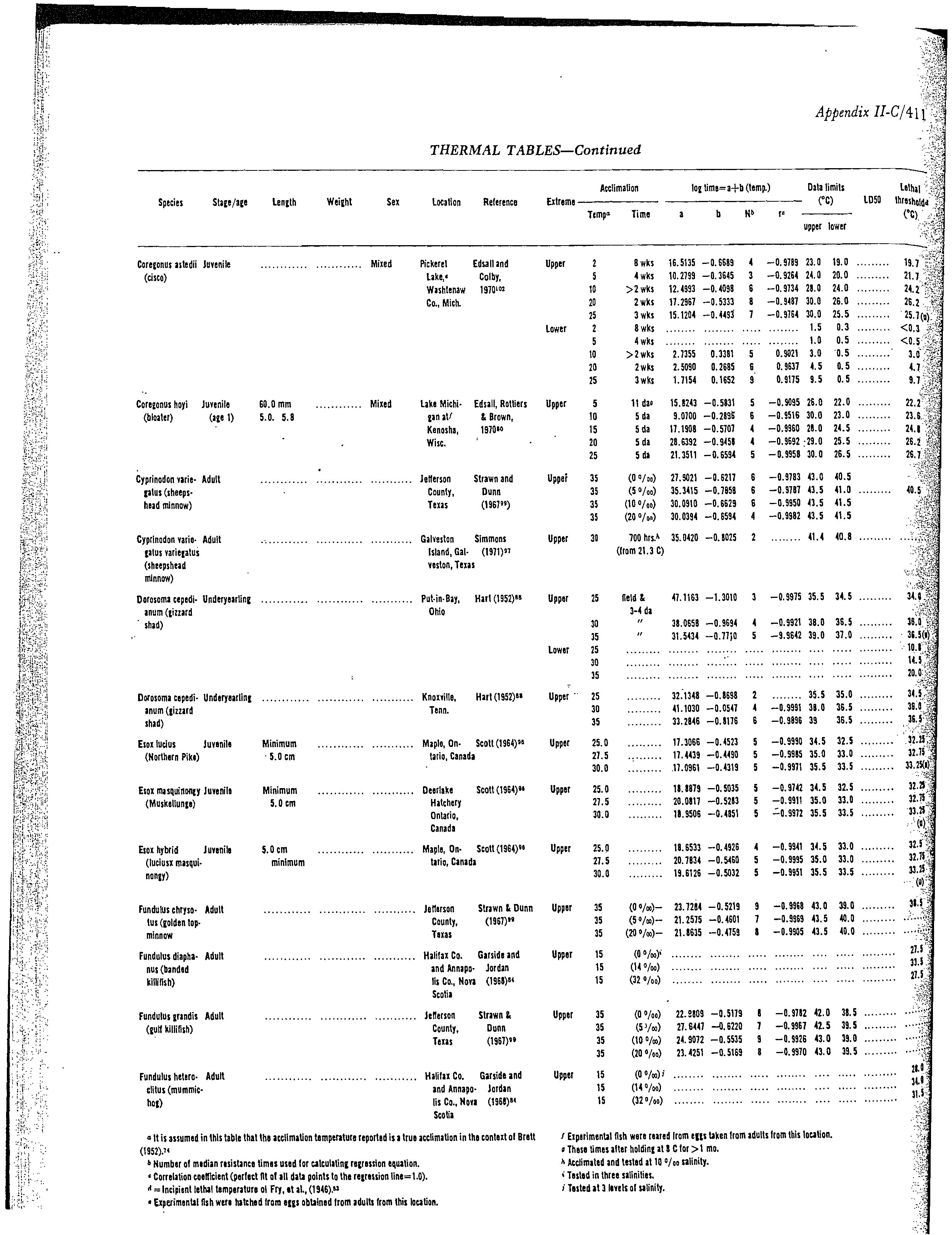
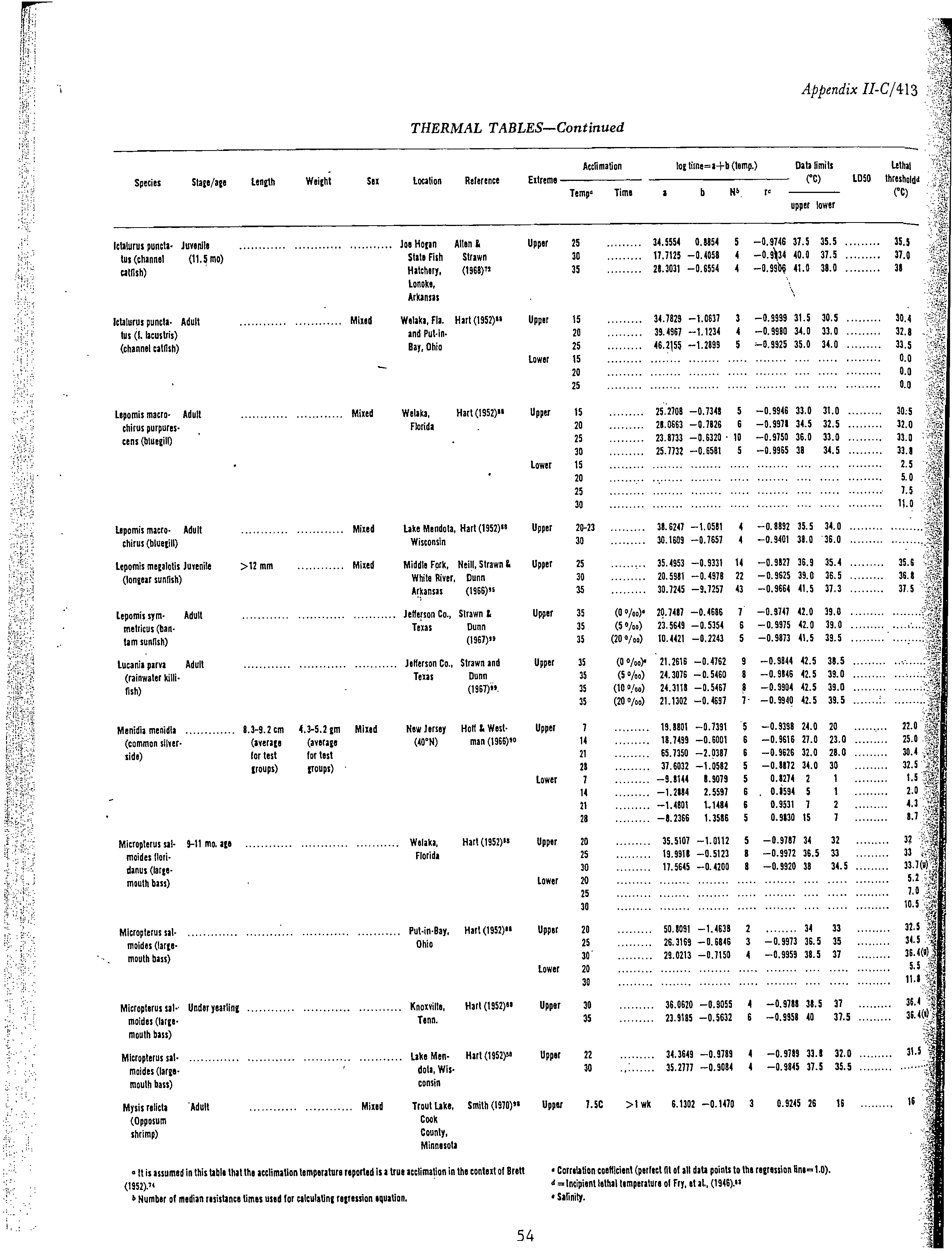
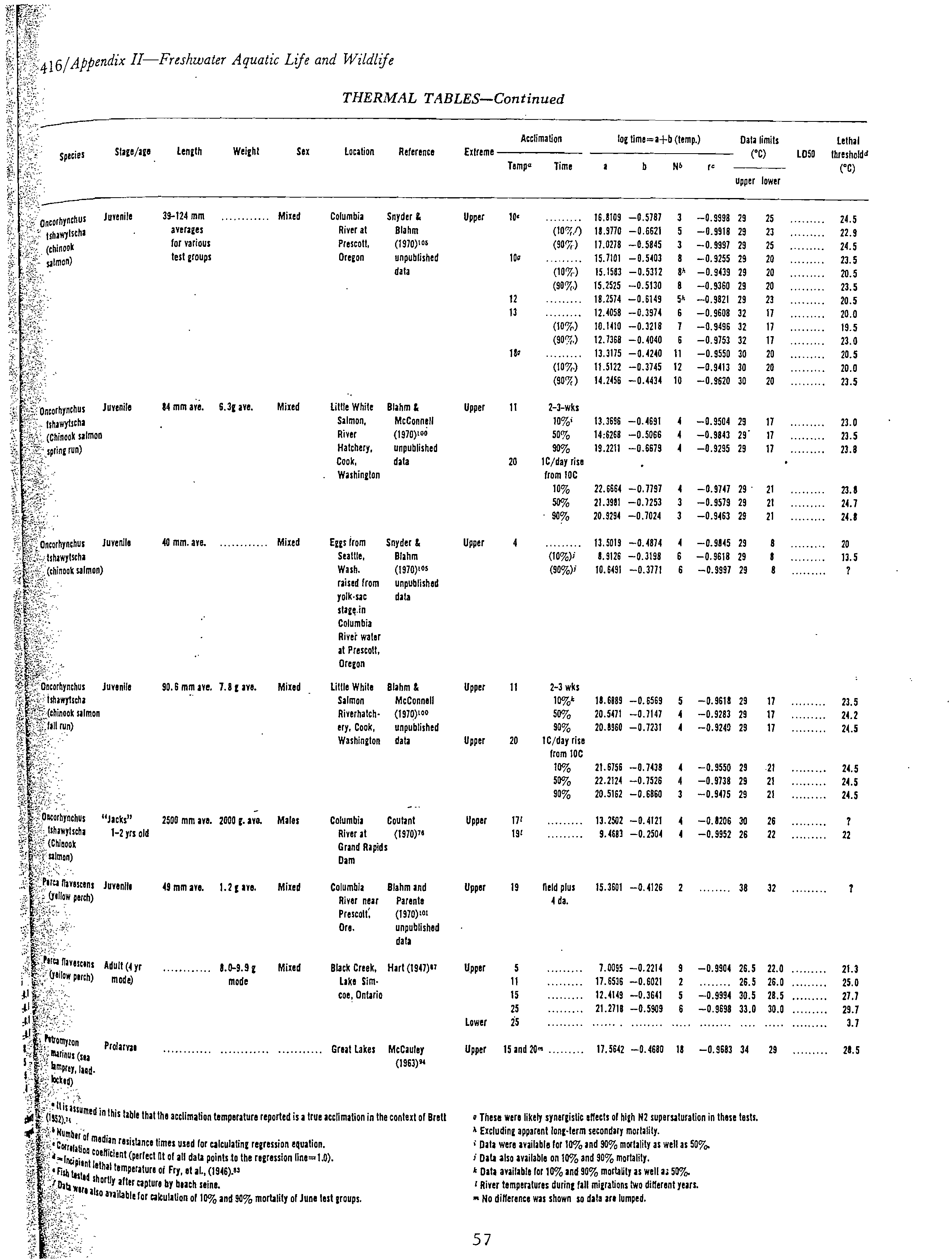
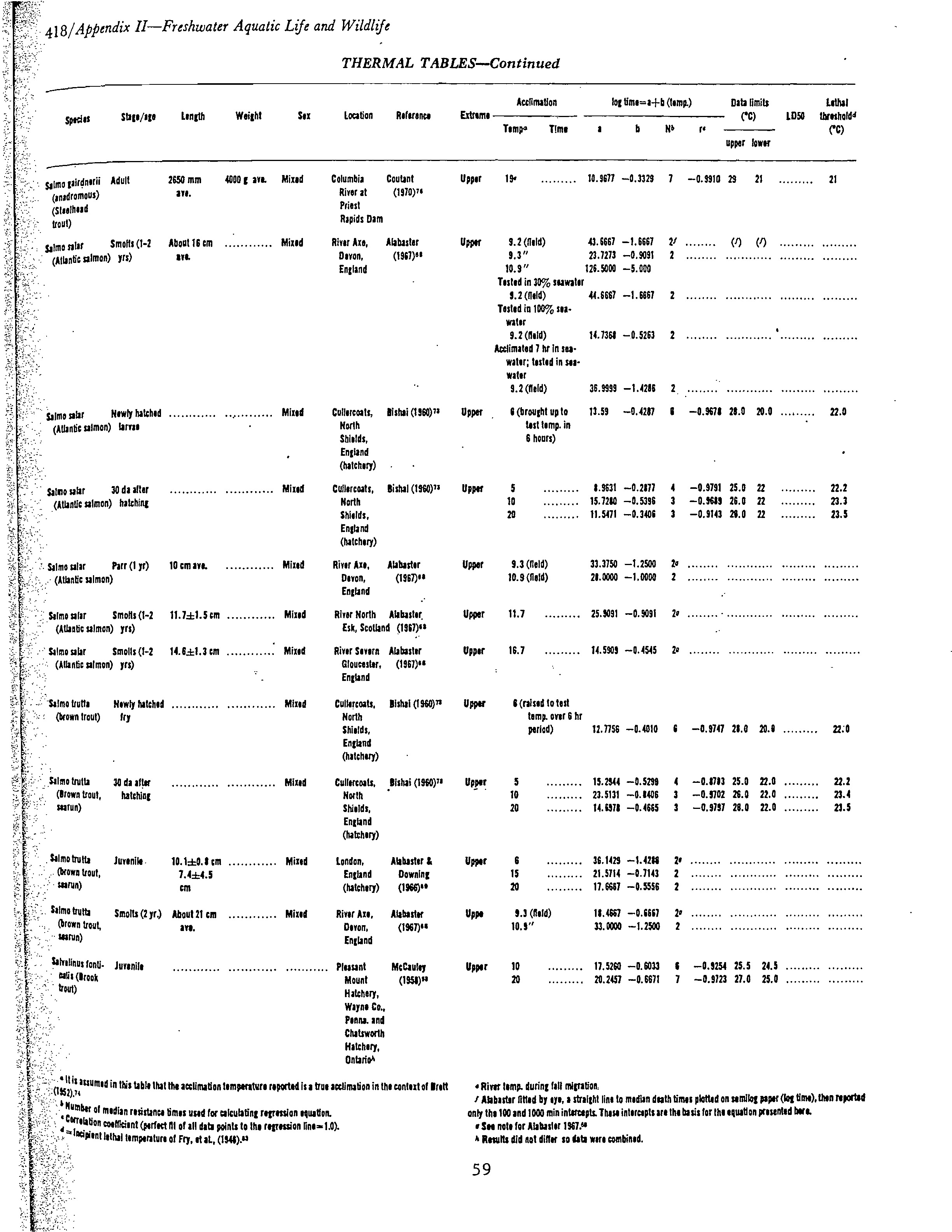
The thermal tables from National Academy of Sciences and

National Academy of Engineering (1973)

?

51

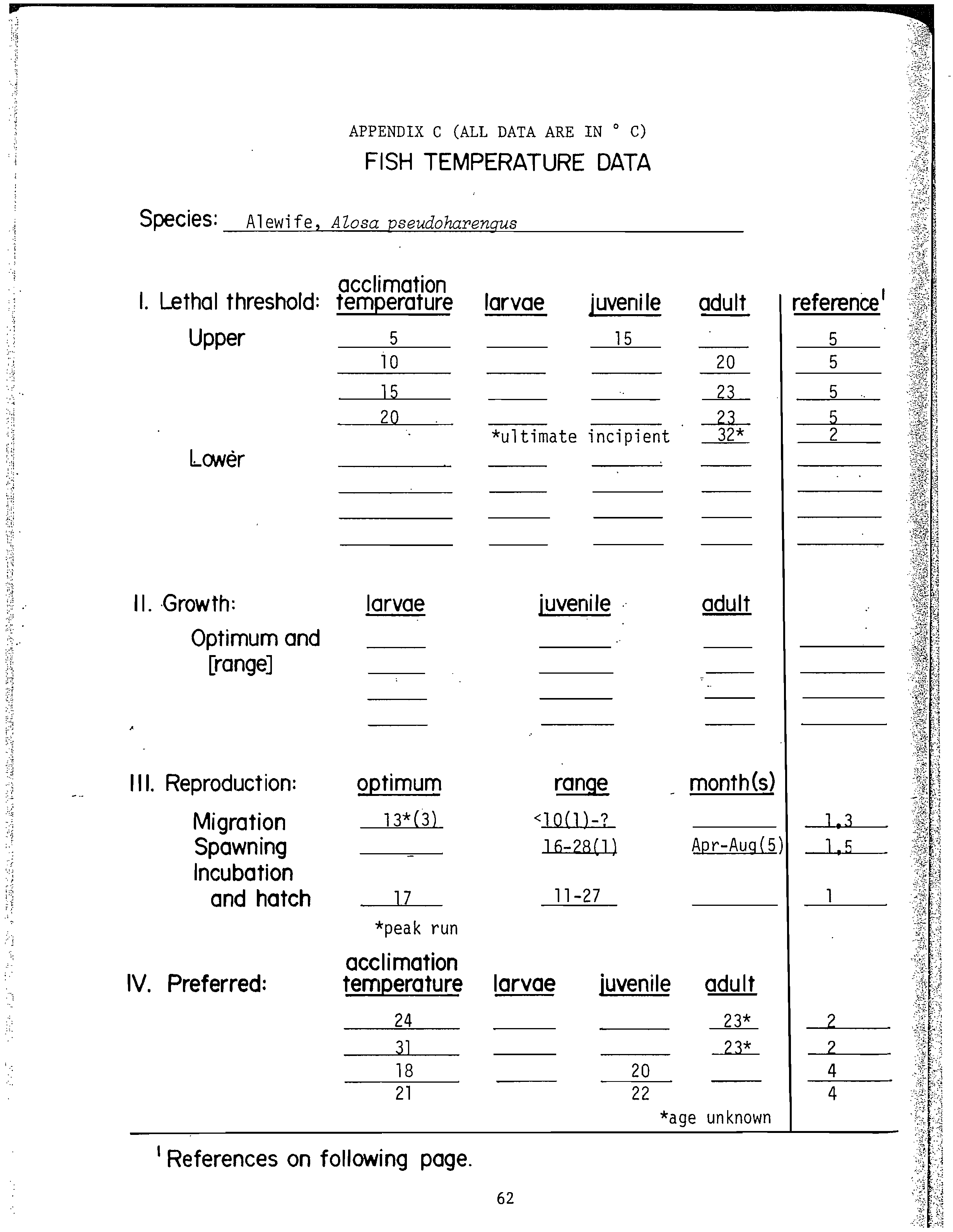
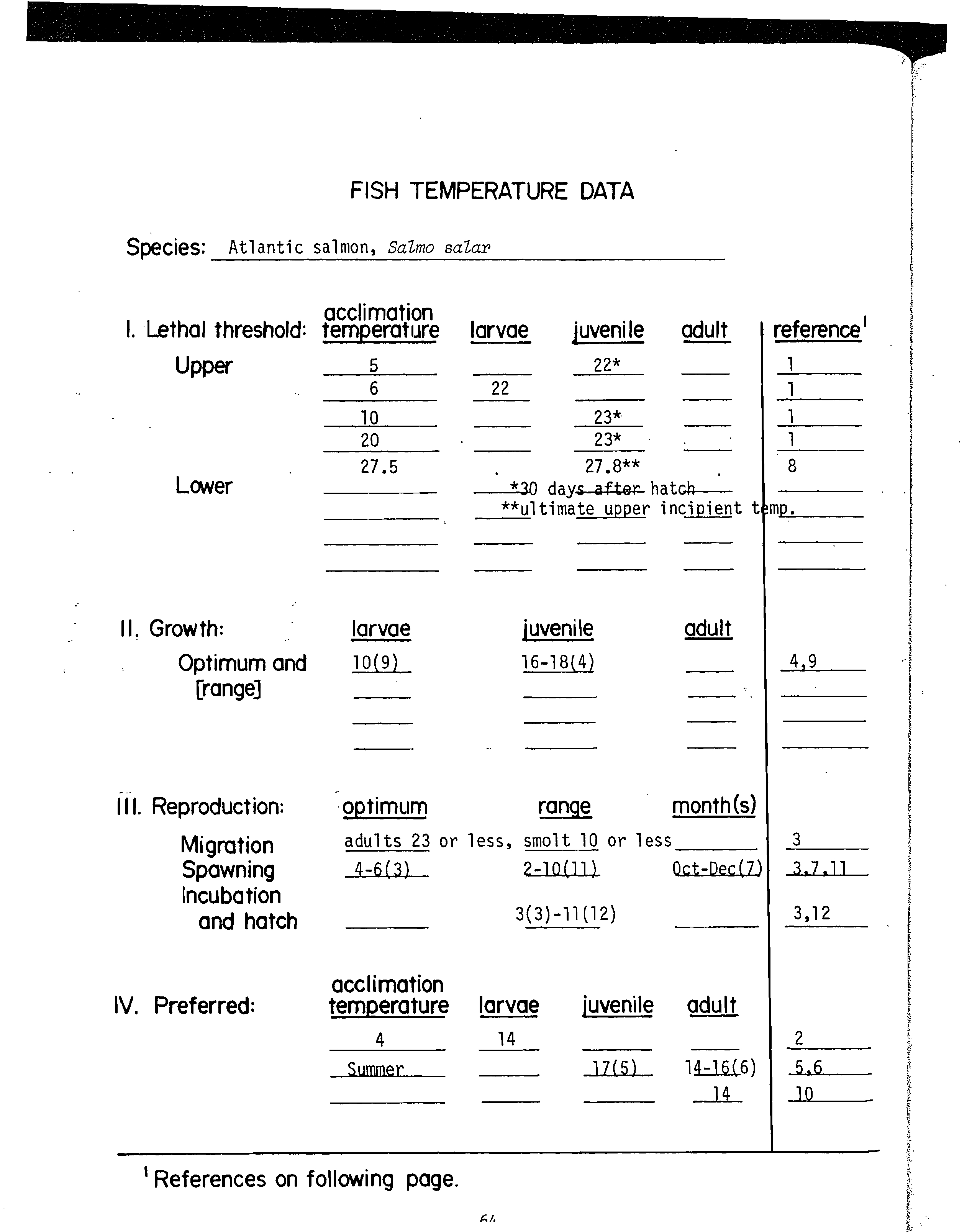
C.

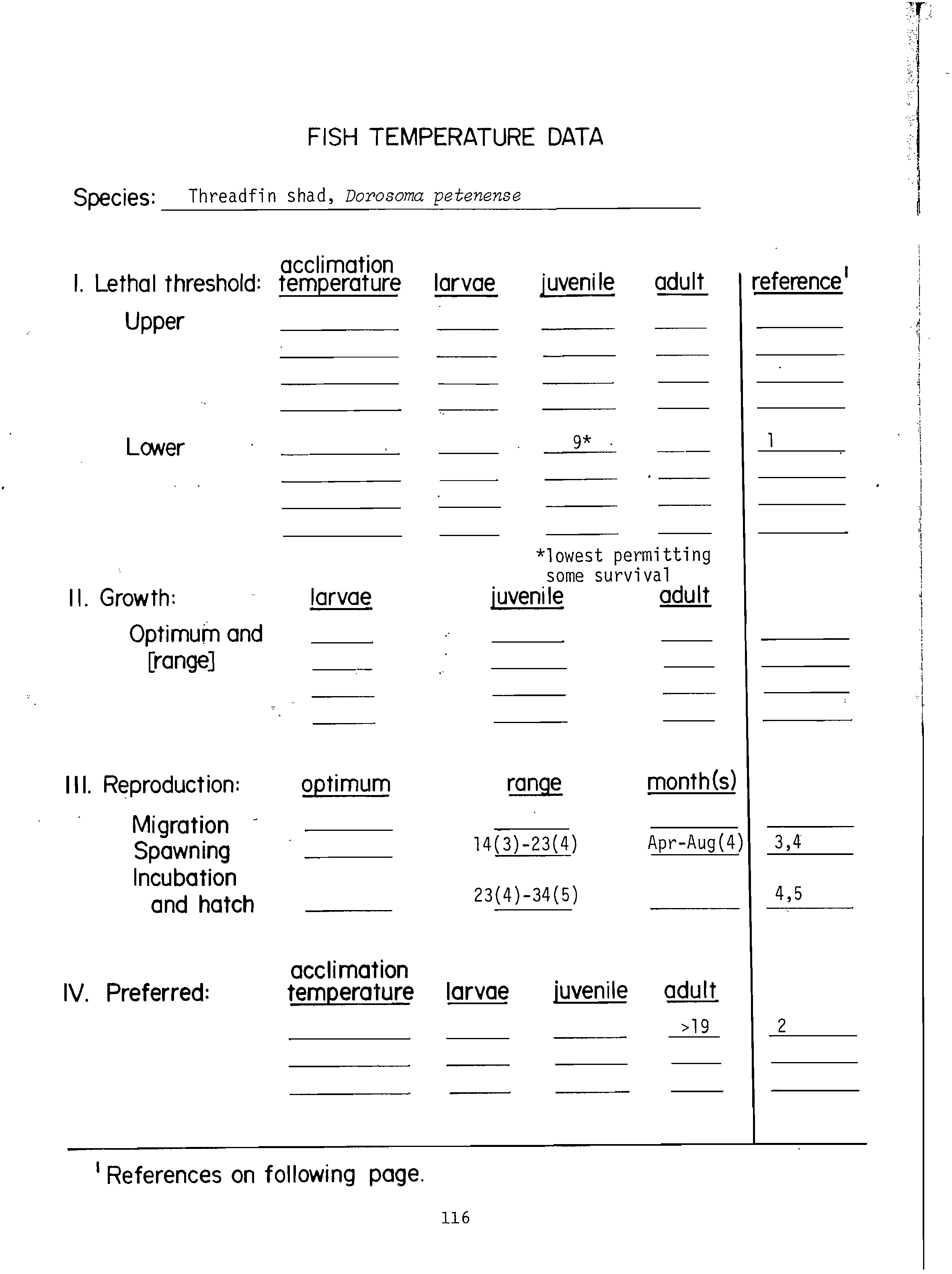
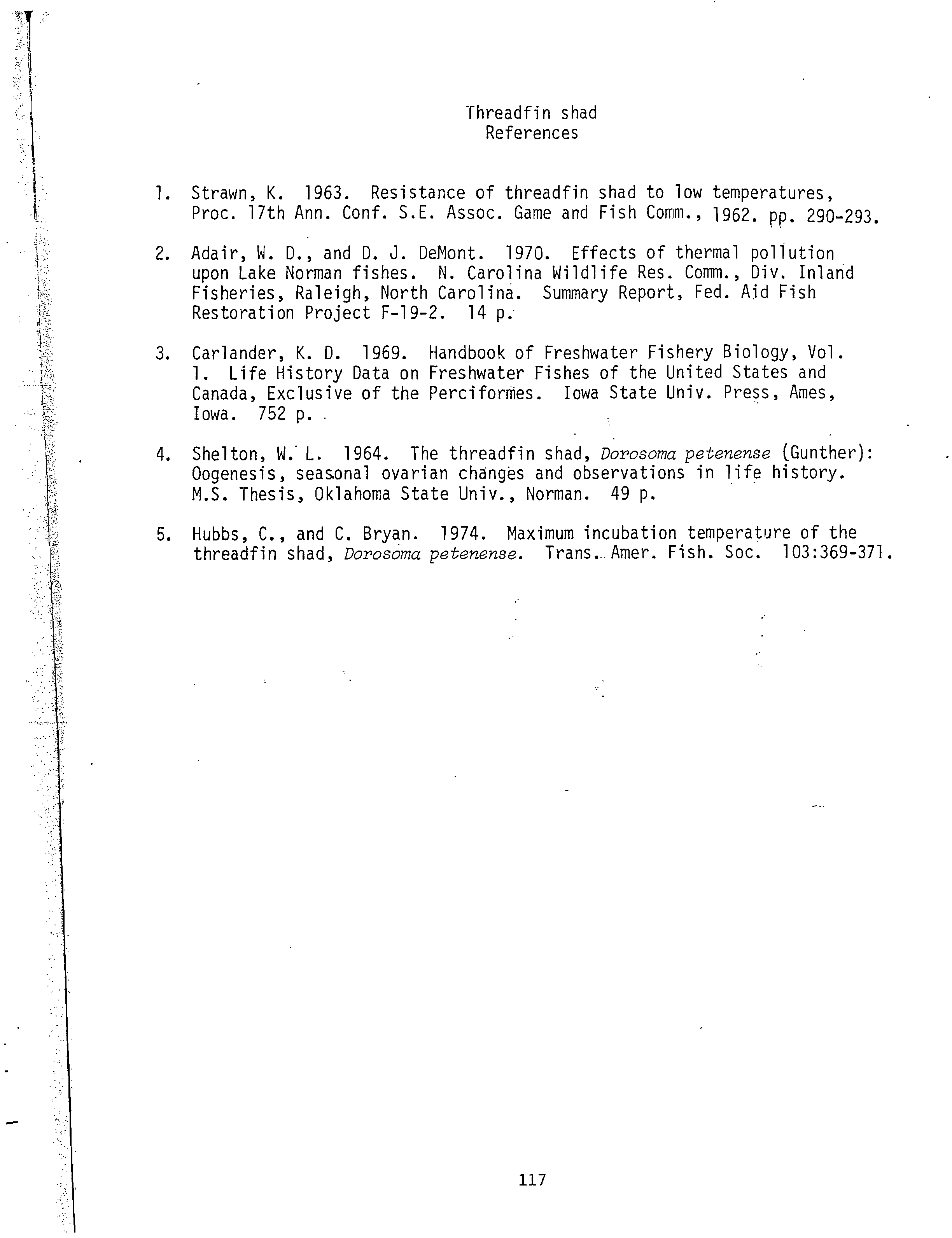
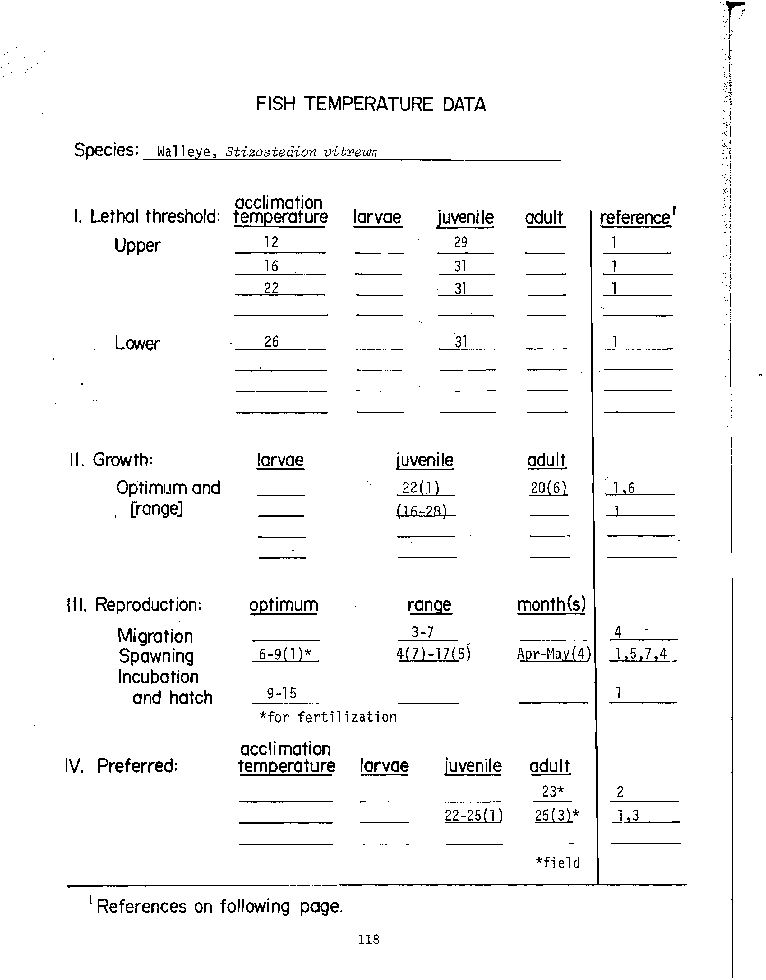
Fish temperature data sheets ?

62

---

ACKNOWLEDGMENTS

We would like to express our appreciation for review of this report to

Dr. Charles C. Coutant (Oak Ridge National Laboratory), Mr. Carlos M.

Fetterolf, Jr. (Great Lakes Fishery Commission), Mr. William L. Klein (Ohio

River Valley Sanitation Commission), and Dr, Donald I. Mount, Dr. Kenneth E. F.

Hokanson and Mr. J. Howard McCormick (Environmental Research Laboratory-

Duluth).

v

i

---

SECTION 1

SUMMARY AND CONCLUSIONS

The evolution of freshwater temperature criteria has advanced from the

search for a single "magic number" to the generally accepted protocol for

determining mean and maximum numerical criteria based on the protection of

appropriate desirable or important fish species, or both. The philosophy and

protocol of the National Academy of Sciences and National Academy of

,

Engineering (1973) were used to determine criteria for survival, spawning,

embryo development, growth, and gamete maturation for species of freshwater

fish, both warmwater and coldwater species.

The influence that management objectives and selection of species have

on the application of temperature criteria

,

is extremely important, especially

if an inappropriate, but very temperature-sensitive, species is included. In

such a case, unnecessarily restrictive criteria will be derived. Conversely,

if the most sensitive important species is not considered, the resultant

criteria will not be protective.

---

SECTION 2

INTRODUCTION

This report is intended to be a guide for derivation of temperature

criteria for freshwater fish based on the philosophy and protocol presented

by the National Academy of Sciences and National Academy of Engineering (1973).

It is not an attempt to gather and summarize the literature on thermal effects.

Methods for determination of temperature criteria have evolved and

developed rapidly during the. past 20 years, making possible a vast increase

in basic data on the relationship of temperature to various life stages.

One of the earliest published temperature criteria for freshwater life

was prepared by the Aquatic Life Advisory Committee of the Ohio River Valley

Water Sanitation Commission (ORSANCO) in 1956. These criteria were based on

conditions necessary to maintain a well-rounded fish population and to sustain

production of a harvestable crop in the Ohio River watershed. The committee

recommended that the temperature of the receiving water:

1)

,

Should not be raised above 34° C (93°F) at any place

or at any time;

should not be raised above 23° C (73° F) at any place

or at any time during the months of December through

April; and

3) should not be raised in streams suitable for trout

propagation.

McKee and Wolf (1963) in their discussion of temperature criteria for the

propagation of fish and other aquatic and marine life refer only to the

progress report of ORSANCO's_Aquatic Life Advisory Committee (.1956).

In 1967 the Aquatic Life Advisory Committee of ORSANCO evaluated and

further modified their recommendations for temperature in the Ohio River

watershed. At this time the committee expanded their recommendation of a

93° F (33.9° C) instantaneous temperature at any time or any place to include

a daily mean of 90° F (32.2° C). This, we believe, was one of the first

efforts to recognize the importance of both mean and maximum temperatures

to describe temperature requirements of fishes. The 1967 recommedations also

included:

Maximum temperature during December, January, and February

should be 55° F (12.8° C);

2

---

2) during the transition months of March, April, October and

November the temperature can be changed gradually by not

more than 7° F (3.9° C);

to maintain trout habitats, stream temperatures should not

exceed 55° F (12.8° C) during the months of October through

May, or exceed 68° F (20.0° C) during the months of June

through September; and

4) insofar as possible the temperature should not be raised

in streams used for natural propagation of trout.

The National Technical Advisory Committee of the Federal Water Pollution

Control Administration presented a report on water quality criteria in 1968

that was to become known as the "Green Book." This large committee included

many of the members of ORSANCO's Aquatic Life Advisory Committee. The committee

members recognized that aquatic organisms might be able to endure a high

temperature for a few hours that could not be endured for a period of days.

They also acknowledged that no single temperature requirement could be applied

to the United States as a whole, or even to one state, and that the requirements

must be closely related to each body of water and its fish populations. Other

important conditions for temperature requirements were that (1) a seasonal cycle

must be retained, (2) the changes in temperature must be gradual, and (3) the

temperature reached must not be so high or so low as to damage or alter the

composition of the desired population. These conditions led to an approach to

criteria development different from earlier ones. A temperature increment

based on the natural water temperature was believed to be more appropriate

than an unvarying number. The use of an increment requires a knowledge of

the natural temperature conditions of the water in question, and the size of

the increment that can be tolerated by the desirable species.

The National Technical Advisory Committee (1968, p. 42) recommended:

"To maintain a well–rounded population of warmwater fishes .... heat

- should not be added to a stream in excess of the amount that will

raise the temperature of the water (at the expected minimum daily

flow for that month) more than 5° F."

A casual reading of this requirement resulted in the unintended generalization

that the acceptable temperature rise in warmwater fish streams was 5° F (2.8°

C). This generalization was incorrect! Upon more careful reading the key

word "amount" of heat and the key phrase "minimum daily flow for that month"

clarify the erroneousness of the generalization. In fact, a 5° F (2.8° C)

rise in temperature could only be acceptable under low flow conditions for a

particular month and any increase in flow would result in a reduced increment

of temperature rise since the amount of heat added could not be increased.

For lakes and reservoirs the temperature rise limitation was 3° F (1.7° C)

based "on the monthly average of the maximum daily temperature."

In trout and salmon waters the recommendations were that "inland trout

streams, headwaters of salmon streams, trout and salmon lakes, and reservoirs

containing salmonids should not be warmed," that "no heated effluents should

3

---

be discharged in the vicinity of spawning areas," and that "in lakes and

reservoirs, the temperature of the hypolimnion should not be raised more

than 3° F (1.7° C)." For other locations the recommended incremental rise

was 5° F (2.8° C) again based on the minimum expected flow for that month.

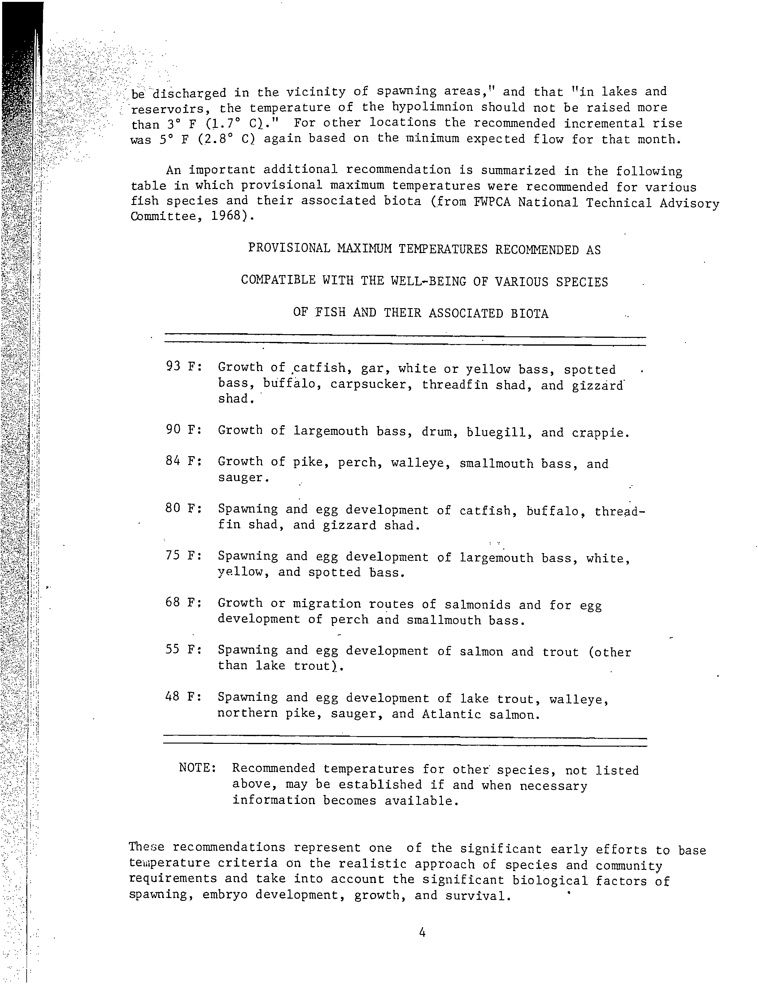
An important additional recommendation is summarized in the following

table in which provisional maximum temperatures were recommended for various

fish species and their associated biota (from FWPCA National Technical Advisory

Committee, 1968).

PROVISIONAL MAXIMUM TEMPERATURES RECOMMENDED AS

COMPATIBLE WITH THE WELL-BEING OF VARIOUS SPECIES

OF FISH AND THEIR ASSOCIATED BIOTA

93 F: Growth of catfish, gar, white or yellow bass, spotted

bass, buffalo, carpsucker, threadfin shad, and

gizzard

shad.

90 F: Growth of largemouth bass, drum, bluegill, and crappie.

84 F: Growth of pike, perch, walleye, smallmouth bass, and

sauger.

80 F; Spawning and egg development of catfish, buffalo, thread-

fin shad, and gizzard shad.

75 F: Spawning and egg development of largemouth bass, white,

yellow, and spotted bass.

68 F; Growth or migration routes of salmonids and for egg

development of perch and smallmouth bass.

55 F: Spawning and egg development of salmon and trout (other

than lake trout).

48 F: Spawning and egg development of lake trout, walleye,

northern pike, sauger, and Atlantic salmon.

NOTE: Recommended temperatures for other species, not listed

above, may be established if and when necessary

information becomes available.

These recommendations represent one of the significant early efforts to base

telaperature criteria on the realistic approach of species and community

requirements and take into account the significant biological factors of

spawning, embryo development, growth, and survival.

?

•

4

---

The Federal Water Pollution Control Administration (1969a) recommended

revisions in water quality criteria for aquatic life relative to the Main

Stem of the Ohio River. These recommendations were presented to ORSANCO's

Engineering Committee and were based on the temperature requirements of

important Ohio River fishes including largemouth bass, smallmouth bass, white

bass, sauger, channel catfish, emerald shiner, freshwater drum, golden

redhorse, white sucker, and buffalo (species was not indicated). Temperature

requirements for survival, activity, final preferred temperature, reproduction,

and growth were considered. The recommended criteria were:

1.

"The water temperatures shall not exceed 90° F

(32.2° C) at any time or any place, and a

maximum hourly average value of 86° F (30° C)

shall not be exceeded."

2.

"The temperature shall not exceed the

temperature values expressed on the following

table:"

AQUATIC LIFE TABLEa

Daily mean

(°

F).

Hourly maximum

(

Q

F)

December-February

48

55

Early March

50

56

Late March

52

58

Early April

55

60

Late April

58

62

Early May

62

64

Late May

68

72

Early June

75

79

Late June

78

82

July-September

82

86

October

75

82

November

65

72

a

From: Federal Water Pollution Control Administration

(1969a).

5

---

The principal limiting fish species considered in developing these criteria

was the sauger, the most temperature sensitive of the important Ohio River

fishes. A second set of criteria (Federal Water Pollution Control

Administration, 1969b) considered less temperature-sensitive species, and the

criteria for mean temperatures were higher. The daily mean in July and

September was 84° F (28.9° C). In addition, a third set of criteria was

developed that was not designed to protect the smallmouth bass, emerald

shiner, golden redhorse, or the white sucker. The July-to-September daily

mean temperature criterion was 86° F (30° C).

The significance of the 1969 Ohio River criteria was that they were

species dependent and that subsequently the criteria would probably be based

upon a single species or a related group of species. Therefore, it is

extremely important to select properly the species that are important otherwise

the criteria will be unnecessarily restrictive. For example, if yellow perch

is an extremely rare species in a water body and is the most temperature-

sensitive species, it probably would be unreasonable to establish temperature

criteria for this species as part of the regulatory mechanism.

In 1970 ORSANCO established new temperature standards that incorporated

the recommendations for temperature criteria of the Federal Water Pollution

Control Administration (1969a, 1969b)

.

and the concept of limiting the amount

of heat that would be added (National Technical Advisory Committee, 1968).

The following is the complete text of that standard:

" All cooling water from municipalities or political

subdivisions, public or private institutions, or

installations, or corporations discharged or

permitted to flow into

,

the Ohio River from the point

of confluence of the Allegheny and Monongahela Rivers

at Pittsburgh, Pennsylvania, designated as

Ohio River

mile point 0.0 to Cairo Point, Illinois, located at

the confluence of the Ohio and Mississippi Rivers, and

being 981.0 miles downstream from Pittsburgh, Pennsylvania,

shall be so regulated or controlled as to provide for

reduction of heat content to such degree that the aggregate

heat-discharge rate from the municipality, subdivision,

institution, installation or corporation, as calculated on

the basis of discharge volume and temperature. differential

(temperature of discharge minus upstream river temperature)

does not exceed the amount calculated by the following

formula, provided, however, that in no case shall the

aggregate heat-discharge rate be of such magnitude as will

result in a calculated increase in river temperature of

more than 5 degrees F:

Allowable heat-discharge rate (Btu/sec) = 62.4 X

river flow (CFS) X (T

a

- T

r

) X 90%

6

---

Where:

T

a

= Allowable maximum temperature (deg. F.)

in the river as specified in the following

table:

January

50

July

89

February

50

August

89.

March

60

September

87

April

70

October

78

May

80.

November

70

June

87

December

57

T

r

= River temperature (daily average in deg. F.I

upstream from the discharge

River flow = measured flow but not less than

critical flow values specified in

the following table:

River reach

?

Critical

flow

From

?

in cfsa

Pittsburgh, Penn.

(mi.

O.0) ?

Willow Is. Dam (161.7)

?

6,500.

Willow Is. Dam (161.7)

?

Gallipolis Dam (279.21

?

7,400

Gallipolis Dam (279.21?

Meldahl Dam (436.21

?

9,700

Meldahl Dam (436.2)?

McAlpine Dam (605.8)

?

11,900

McAlpine Dam (605.8)

?

Uniontown Dam (846.0)

?

14,200

Uniontown Dam (846.0)

?

Smithland Dam (918.51

?

19,500

Smithland Dam (918.5)

?

Cairo Point (981.0)

?

48,100

a

Minimum daily flow once in ten years.

7

---

Although the numerical criteria for January through December are higher

than those recommended by the Federal Water Pollution Control Administration,

they are only used to calculate the amount of heat that can be added at the

"minimum daily flow once in ten years." Additional flow would result in

lower maxima since no additional heat could be added. There was also the

increase of 5° F (2.8° C) limit that could be more stringent than the maximum

temperature limit.

The next important step in the evolution of thought on temperature

criteria was Water Quality Criteria 1972 (NAS/NAE, 1973), which is becoming

known as the "Blue Book," because of its comparability to the Green Book (FWPCA

National Technical Advisory Committee, 1968). The Blue Book is the report of

the Committee on Water Quality Criteria of the National Academy of Sciences at

the request of and funded by the U.S. Environmental Protection Agency (EPA).

The heat and temperature section, with its recommendations and appendix data,

was authored by Dr. Charles Coutant of the Oak Ridge National Laboratory. These

materials are reproduced in full in Appendix A and Appendix B in this report.

A discussion and description of the Blue Book temperature criteria will be

found later in this report.

The Federal Water Pollution Control Act Amendments of 1972 (Public

Law 92-500) contain a section [304 (al

C11]

that requires that the

administrator of the EPA "after

. consultation with appropriate Federal and

State agencies and other interested persons, shall develop and publish,

within one year after enactment of this title (and from time to time

thereafter revise) criteria for water'quality accurately reflecting the

latest scientific knowledge (A), on the kind and extent of

ell

identifiable

effects on health and welfare including, but not limited tb, plankton,

fish, shellfish, wildlife, plant life, shorelines, beaches, esthetics, and

recreation which may be expected from the

.

presence of pollutants in any

body of water, including ground water; (B) on the concentration and dispersal

of pollutants or their byproducts, through biological, physical, and

chemical processes; and (C) on the effects of pollutants on biological

community diversity, productivity, and stability, including information on

the factors affecting rates of eutrophication and rates of organic and

inorganic sedimentation for varying types of receiving waters."

The U.S. Environmental Protection Agency (1976) has published Quality

Criteria for Water as a response to the Section 304(a)(1) requirements of

PL 92-500. That approach to-the determination of temperature criteria for

freshwater fish is essentially the same as the approach recommended in the

Blue Book (NAS/NAE, 1973). The EPA criteria report on temperature included

numerical criteria for freshwater fish species and a nomograph for winter

temperature criteria. These detailed criteria were developed according

to the protocol in the Blue Book, and the procedures used to develop those

criteria will be discussed in detail in this report.

The Great Lakes Water Quality Agreement (1972) between the United States

of America and Canada was signed in 1972 and contained a specific water

quality objective for temperature. It states that "There should be no change

that would adversely affect any local or general use of these waters." The

8

---

International Joint Commission was designated to assist in the implementation

of this agreement and to give advice and recommendations to both countries

on specific water quality objectives. The International Joint Commission

committees assigned the responsibility of developing these objectives have

recommended temperature objectives for the Great Lakes based on the "Blue

Book" approach and are in the process of refining and completing those

objectives for consideration by the commission before submission to the two

countries for implementation.

A

se

---

SECTION 3

THE PROTOCOL FOR TEMPERATURE CRITERIA

This section is a synthesis of concepts

.

and definitions from Fry et al.

(1942, 1946), Brett (1952, 1956), and the NAS/NAE (1973).

The lethal threshold temperatures are those temperatures at which 50

percent of a sample of individuals would survive indefinitely after acclimation

at some other temperature. The majority of the published literature (Appendix

B) is calculated on the basis of 50 percent survival. These lethal thresholds

are commonly referred to as incipient lethal temperatures. Since organisms

can be lethally stressed by both rising and falling temperatures, there are

upper incipient lethal temperatures and lower incipient lethal temperatures.

These are determined by removing the organisms from a temperature to which

they are acclimated and instantly placing them in a series of other temperatures

that will typically result in a range in survival from 100 to 0 percent.

Acclimation can require up to 4 weeks, depending upon the magnitude of the

difference between the temperature when the fish were obtained and the desired

acclimation temperature, In general, experiments to determine incipient

lethal temperatures should extend until all the organisms in any test chamber

are dead or sufficient time has elapsed for death to have occurred, The

ultimate upper incipient lethal temperature is that beyond which no increase

in lethal temperature is accomplished by further increase in acclimation

temperature. For most freshwater fish species in temperate latitudes the

lower incipient lethal temperatures will usually end at 0° C, being limited

by the freezing point of water. However, for some important species, such as

threadfish shad in freshwater and menhaden in seawater, the lower incipient

lethal temperature is higher than 0° C,

As indicated earlier, the heat and temperature section of the Blue Book

and its associated appendix data and references have been reproduced in this

report as Appendix A and Appendix B. The following discussion will briefly

summarize the various types of criteria and provide some additional insight

into the development of numerical criteria. The Blue Book (Appendix A)

also describes in detail the use of the criteria in relation to entrainment.

MAXIMUM WEEKLY AVERAGE TEMPERATURE

For practical reasons the maximum weekly average temperature (MWAT) is

the mathematical mean of multiple, equally spaced, daily temperatures over a

7-day consecutive period.

10

---

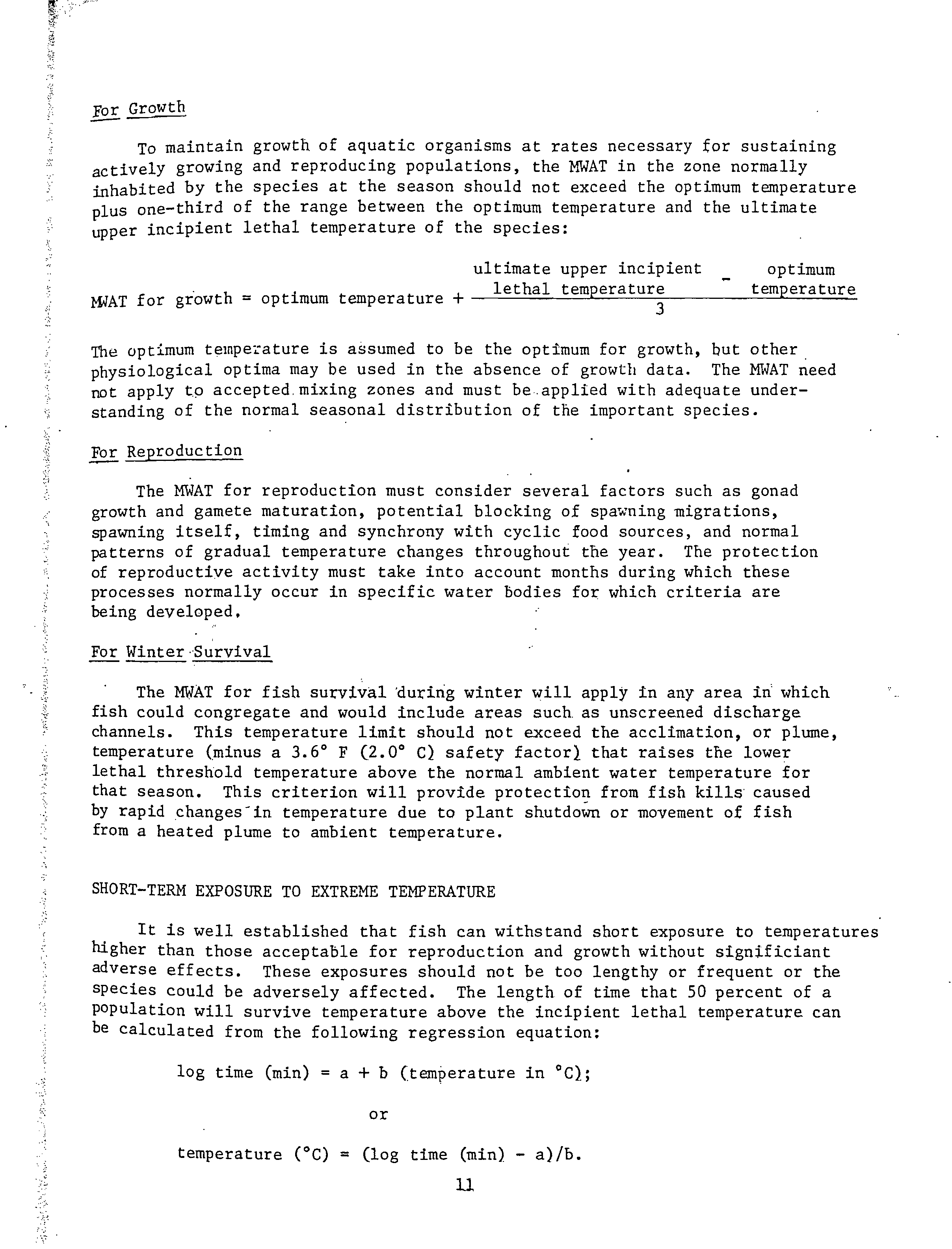
For Growth

To maintain growth of aquatic organisms at rates necessary for sustaining

actively growing and reproducing populations, the MWAT in the zone normally

inhabit

ed

by the species at the season should not exceed the optimum temperature

plus one-third of the range between the optimum temperature and the ultimate

upper incipient lethal temperature of the species:

ultimate upper incipient?

optimum

?MAT for growth = optimum temperature + lethal temperature

?temperature

3

The optimum temperature is assumed to be the optimum for growth, but other

physiological optima may be used in the absence of growth data. The MWAT need

not apply to accepted mixing zones and must be applied with adequate under-

standing of the normal seasonal distribution of the important species.

For Reproduction

The MWAT for reproduction must consider several factors such as gonad

growth and gamete maturation, potential blocking of spawning migrations,

spawning itself, timing and synchrony with cyclic food sources, and normal

patterns of gradual temperature changes throughout the year. The protection

of reproductive activity must take into account months during which these

processes normally occur in specific water bodies for which criteria are

being developed.

For Winter Survival

The MWAT for fish survival during winter will apply in any area in which

fish could congregate and would include areas such as unscreened discharge

channels. This temperature limit should not exceed the acclimation, or plume,

temperature (minus a 3.6° F (2,0° C) safety factor) that raises the lower

lethal threshold temperature above the normal ambient water temperature for

that season. This criterion will provide protection from fish kills caused

by rapid changes

- in temperature due to plant shutdown or movement of fish

from a heated plume to ambient temperature.

SHORT-TERM EXPOSURE TO EXTREME TEMPERATURE

It is well established that fish can withstand short exposure to temperatures

higher than those acceptable for reproduction and growth without significiant

adverse effects. These exposures should not be too lengthy or frequent or the

species could be adversely affected. The length of time that 50 percent of a

population will survive temperature above the incipient lethal temperature can

be calculated from the following regression equation:

log time (min) = a + b (temperature in °C);

or

temperature (°C) = (log time (min) - a)/b.

---

The constants "a" and "b" are for intercept and slope and will be discussed

later. Since this equation is based on 50 percent survival, a 3.6° F (2.0° Cl

reduction in the upper incipient lethal temperature will provide the safety

factor to assure no deaths.

For those interested in more detail or the rationale for these general

criteria, Appendices A and B should be read thoroughly. In addition, Appendix

A contains a fine discussion of a procedure to evaluate the potential thermal

impact of aquatic organisms entrained in cooling water or the discharge

plume, or both.

12

---

SECTION 4

THE PROCEDURES FOR CALCULATING NUMERICAL

TEMPERATURE CRITERIA FOR FRESHWATER FISH

MAXIMUM WEEKLY AVERAGE TEMPERATURE

The necessary minimum data for the determination of this criterion are

the physiological optimum temperature and the ultimate upper incipient lethal

temperature, The latter temperature represents the "breaking point" between

the highest temperatures to which an animal can be acclimated and the lowest

of the extreme upper temperatures that will kill the warm-acclimated organism.

Physiological optima can be based on performance, metabolic rate, temperature

preference, growth, natural distribution, or tolerance. However, the most

sensitive function seems to be growth rate, which appears to be an integrator

of all physiological responses of an organism, In the absence of data on

optimum growth, the use of an optimum for a more specific function related to

activity and metabolism may be more desirable than not developing any growth

criterion at all,

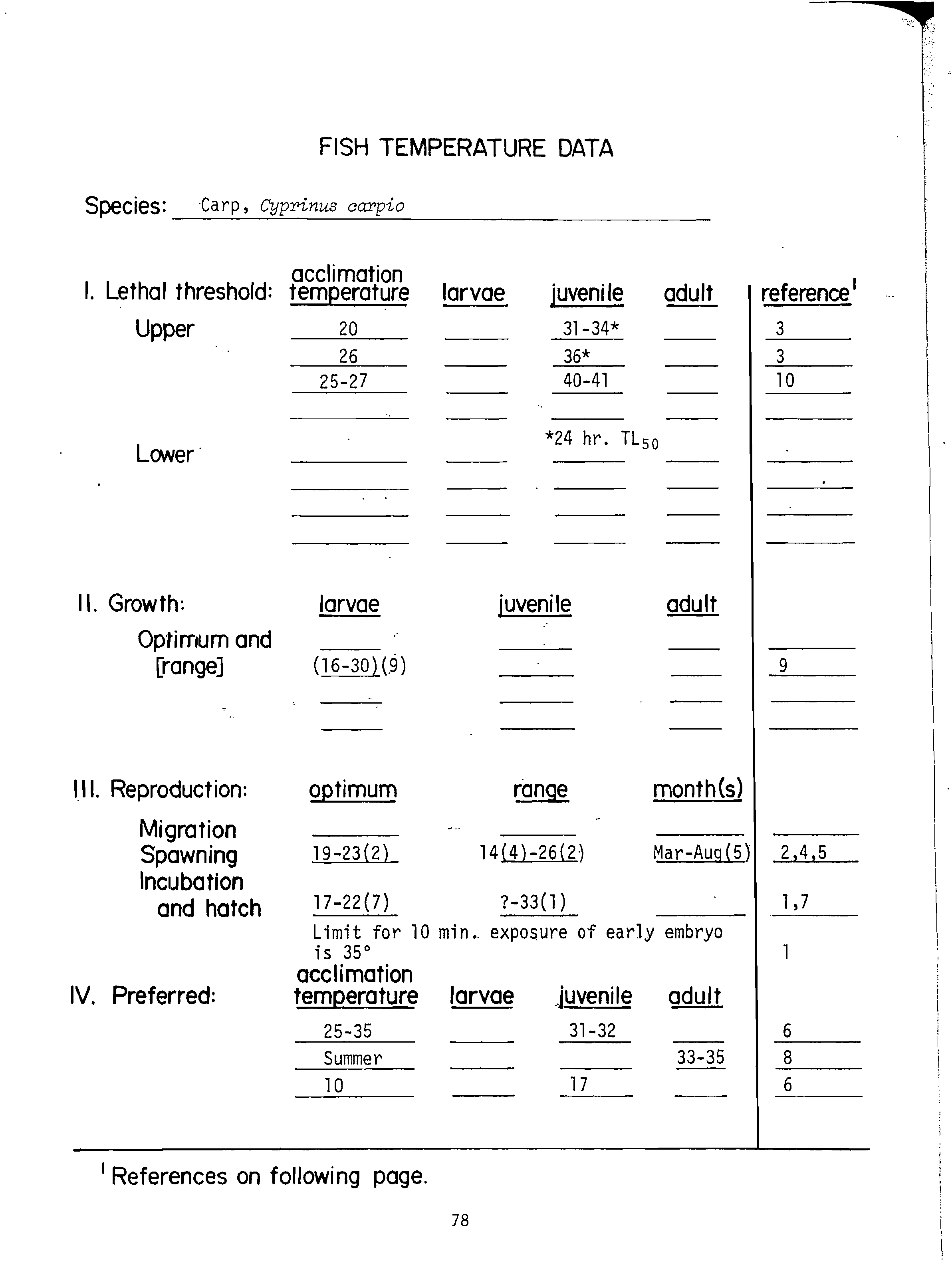
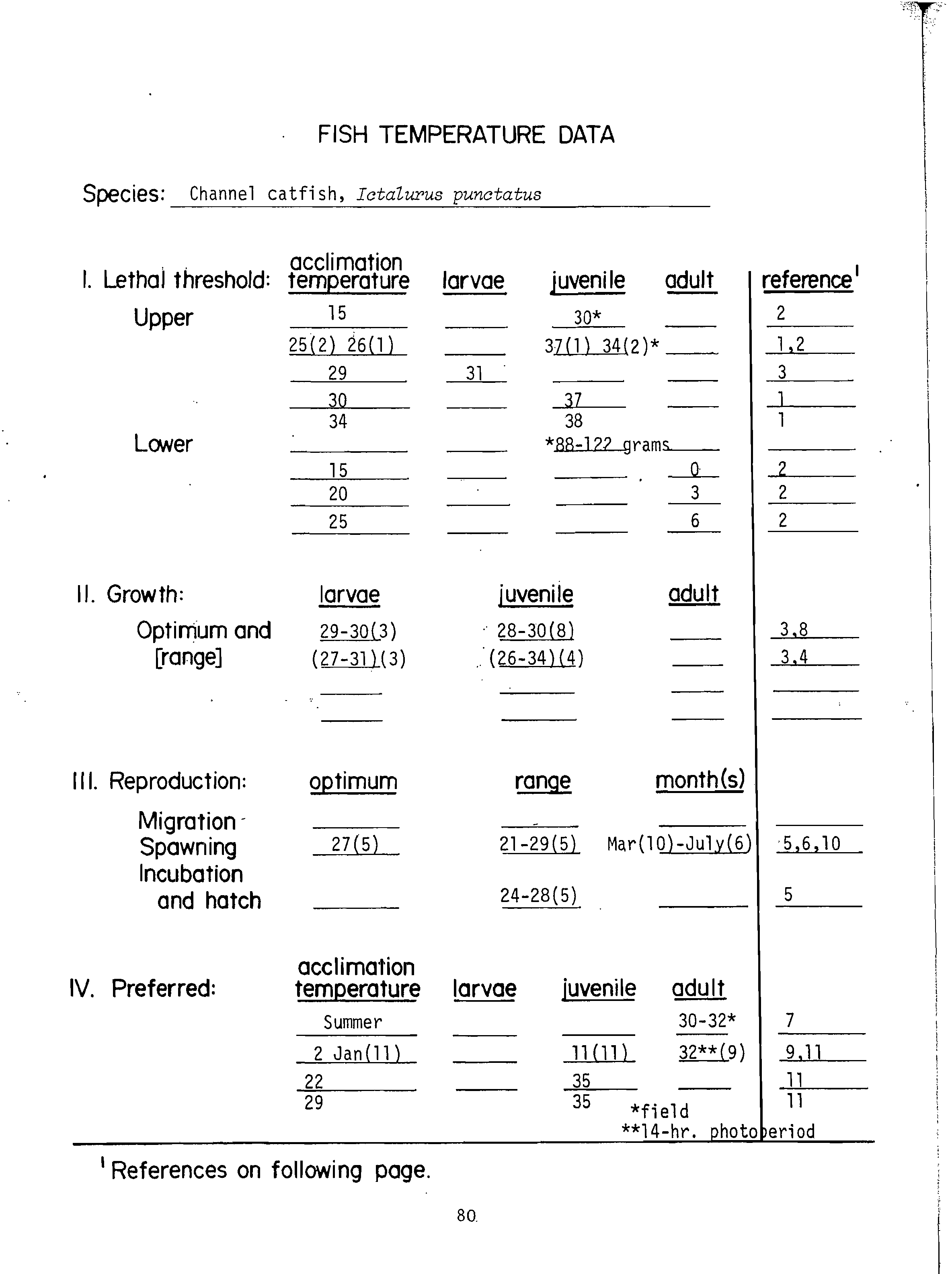
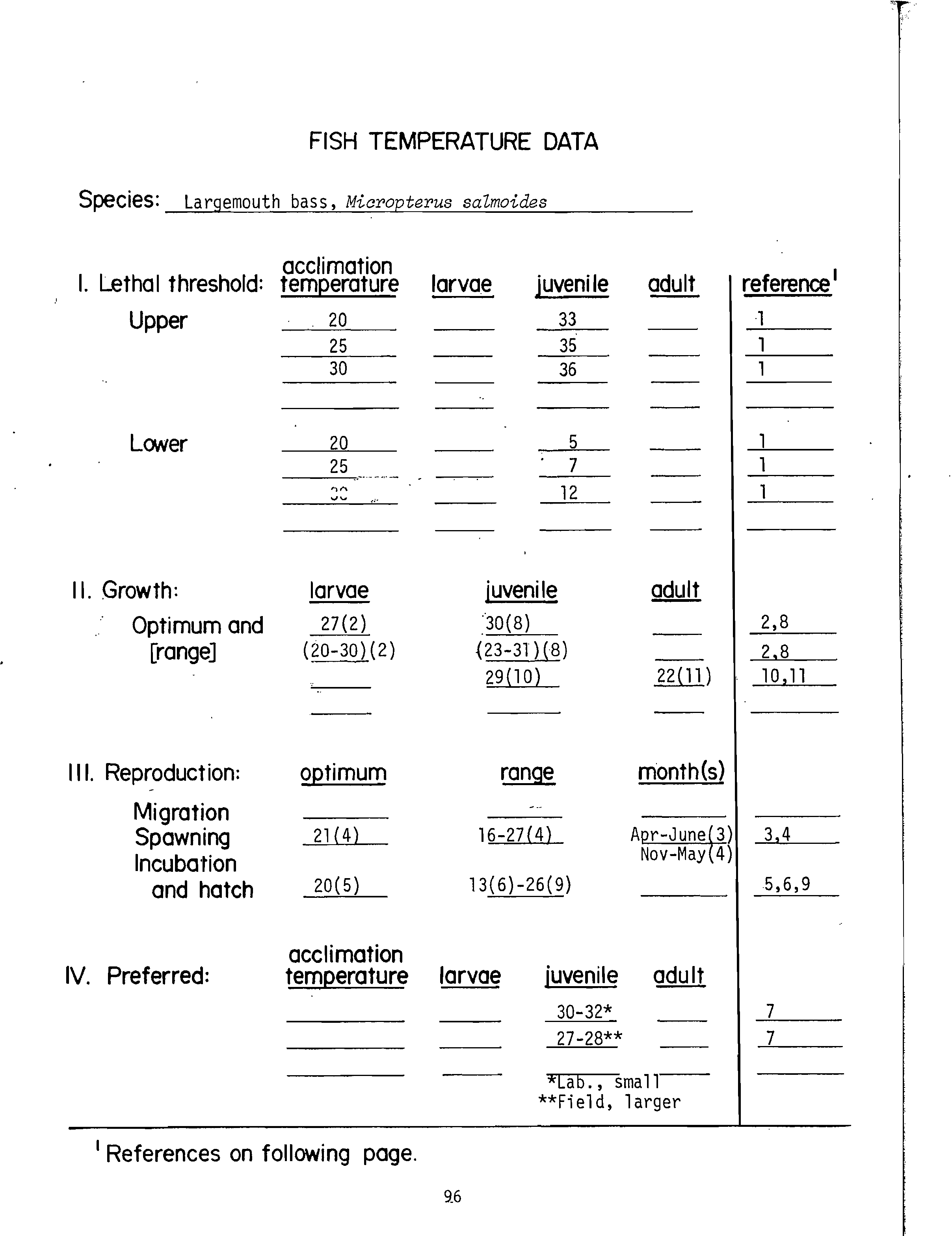
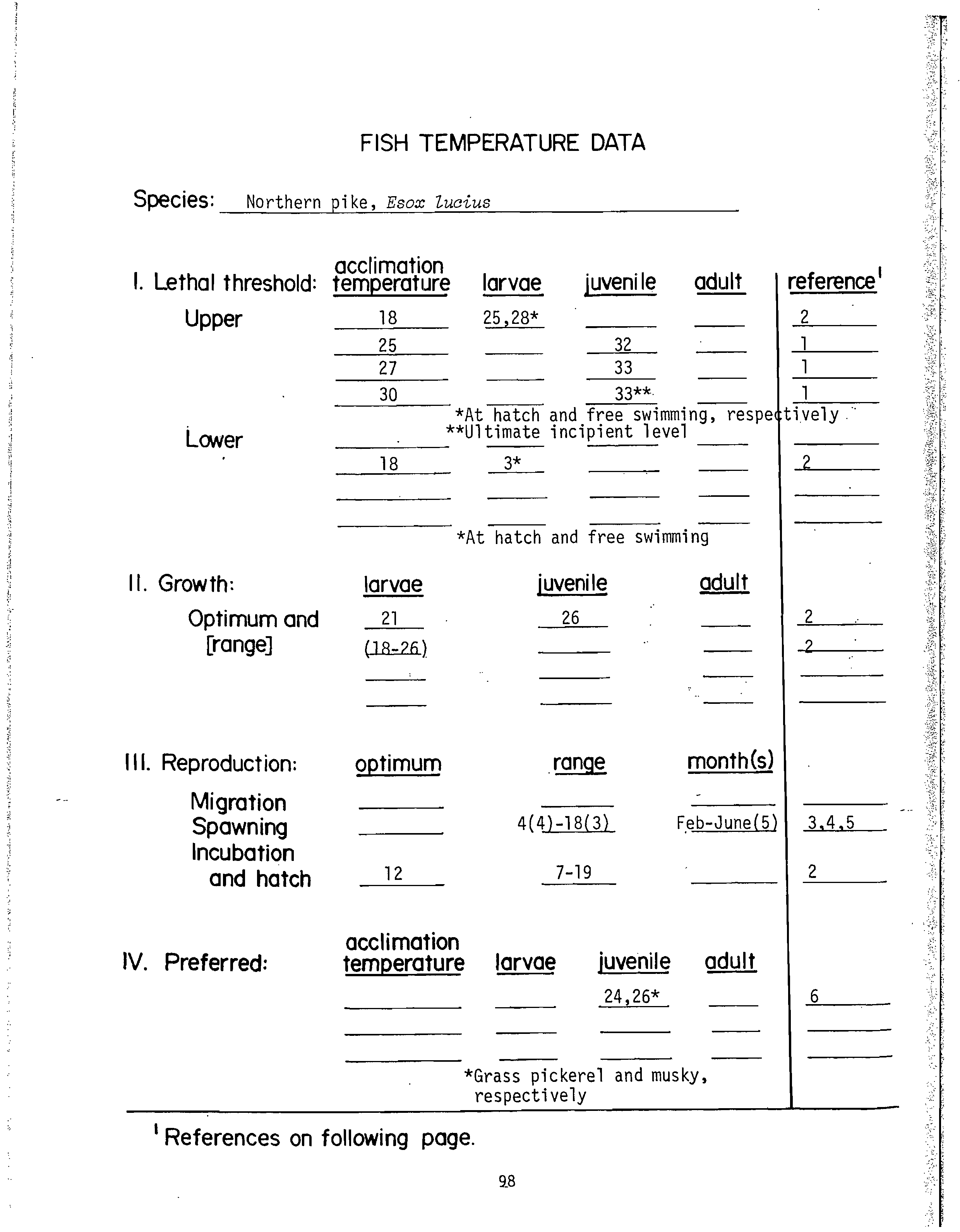
The MWAT's for growth were calculated for fish species for which appropriate

data were available (Table 1). These data were obtained from the fish temperature

data in Appendix C. These data sheets contain the majority of thermal effects

data for about 34 species of freshwater fish and the sources of the data. Some

subjectivity is inevitable and necessary because of variability in published

data resulting from differences in age, day length, feeding regime, or methodology.

For example, the-data sheet for channel catfish (Appendix C) includes four

temperature ranges for optimum growth based on three published papers.' It would

be. more appropriate to use data for growth of juveniles and adults rather than

larvae. The middle of each range for juvenile channel catfish growth is 29° and

30° C. In this instance 29° C is judged the best estimate of the optimum. The

highest incipient lethal temperature (that would approximate the ultimate

incipient lethal temperature) appearing in Appendix C is 38° C. By using the

previous formula for the MWAT for growth, we obtain

29° C +

(38-29°

3

C)

= 32° C.

The temperature criterion for the MWAT for growth of channel catfish would be

32° C (as appears in Table 1).

13

---

TABLE 1. TEMPERATURE CRITERIA FOR GROWTH AND SURVIVAL OF SHORT EXPOSURES

(24 HR) OF JUVENILE AND ADULT FISH DURING THE SUMMER (° C (° F))

Species

Maximum weekly average

temperature for growth

s

Maximum temperature for

survival of short exposure

Alewife

--

Atlantic salmon

20 (68)

23 .(73)

Bigmouth buffalo

--

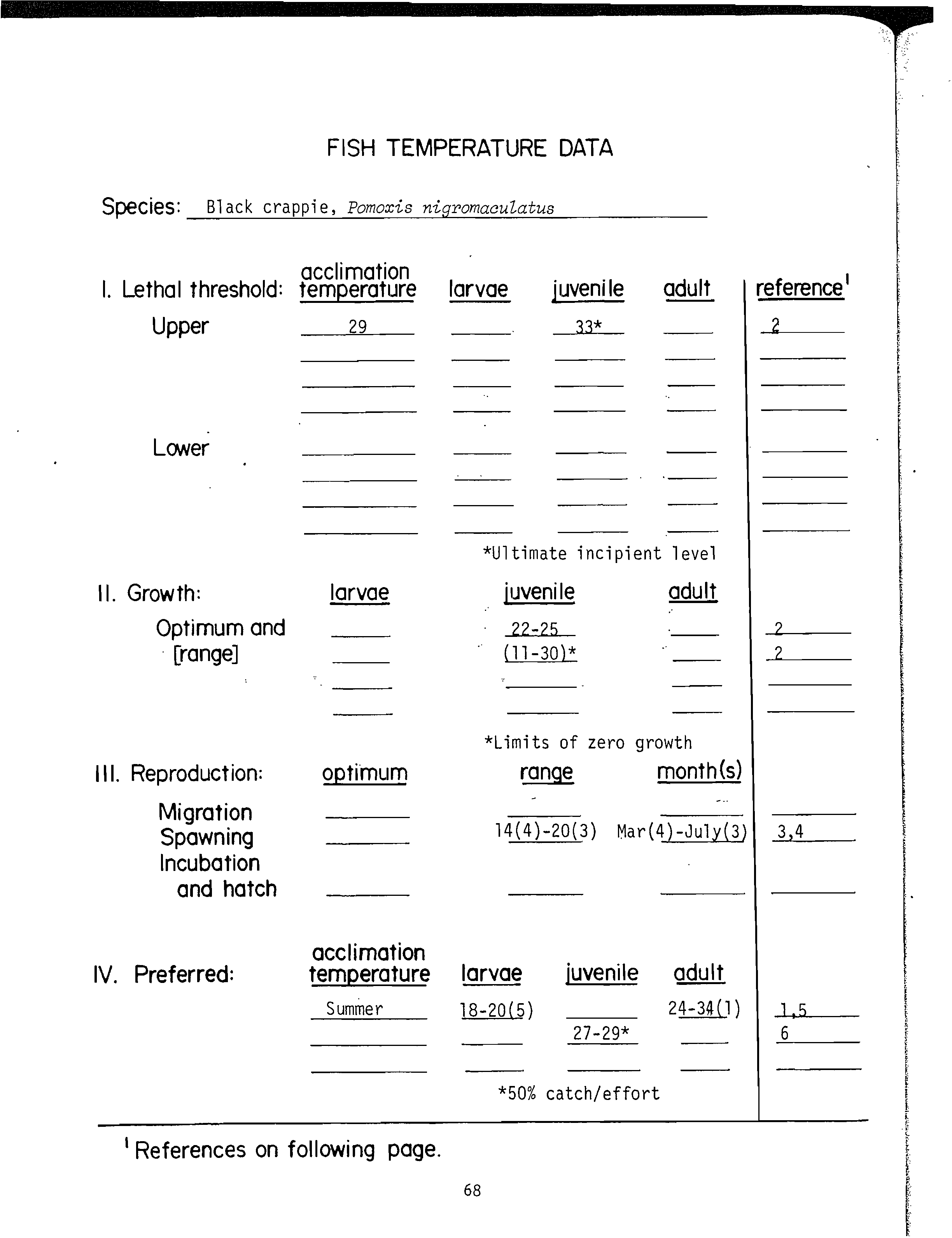
Black crappie

27 (81)

Bluegill

32 (90)

35 (95)

Brook trout

19 (66)

24

(75)

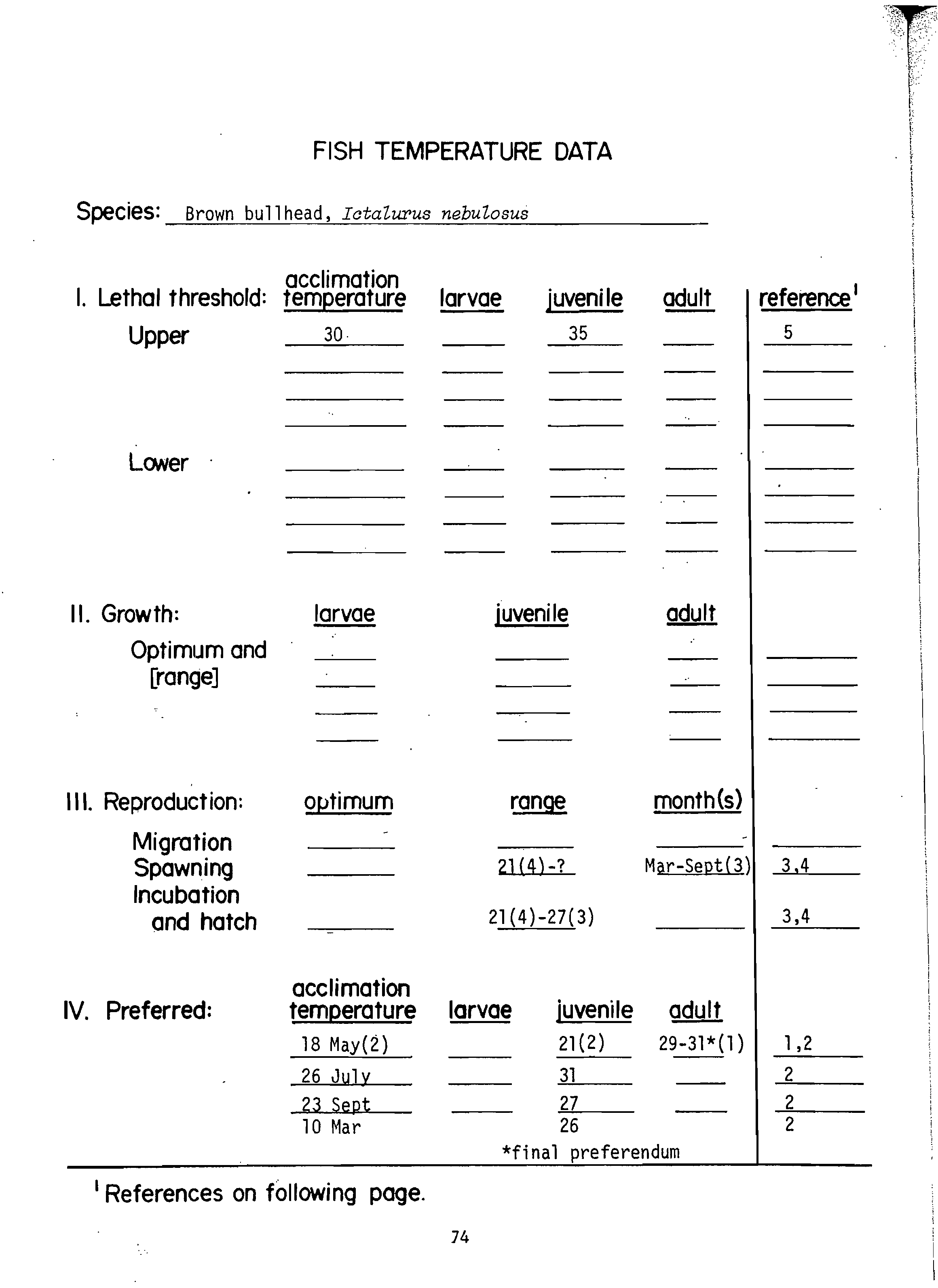
Brown bullhead

' --

Brown trout

17

(63)

24

(75)

Carp

--

Channel catfish

32

(90)

35 (95)

Coho salmon

18

(64)

24

(75)

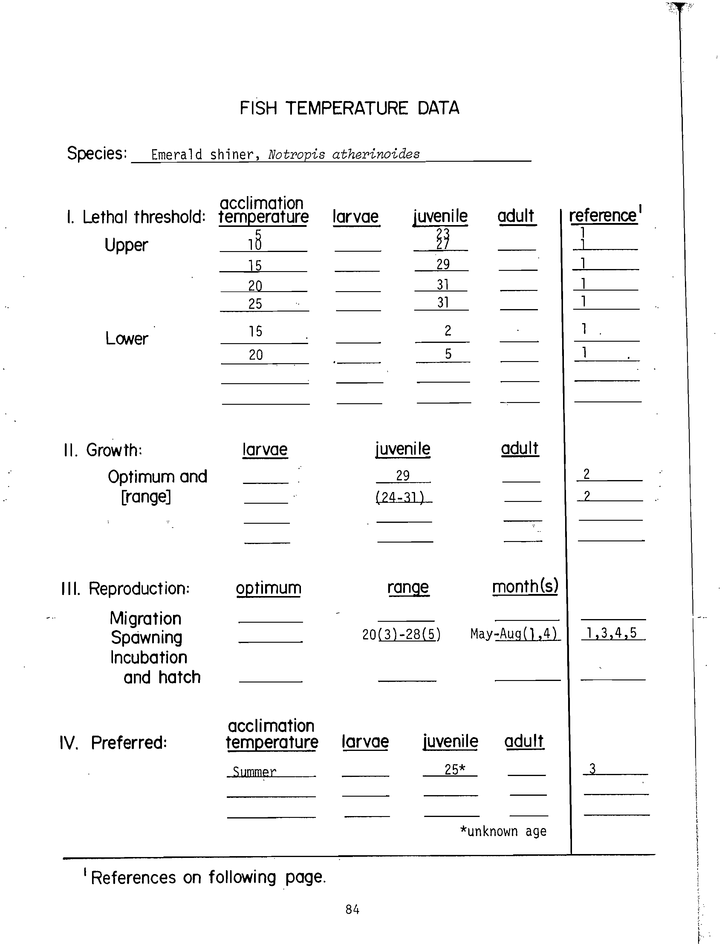
Emerald shiner

30

(86)

Fathead minnow

Freshwater drum

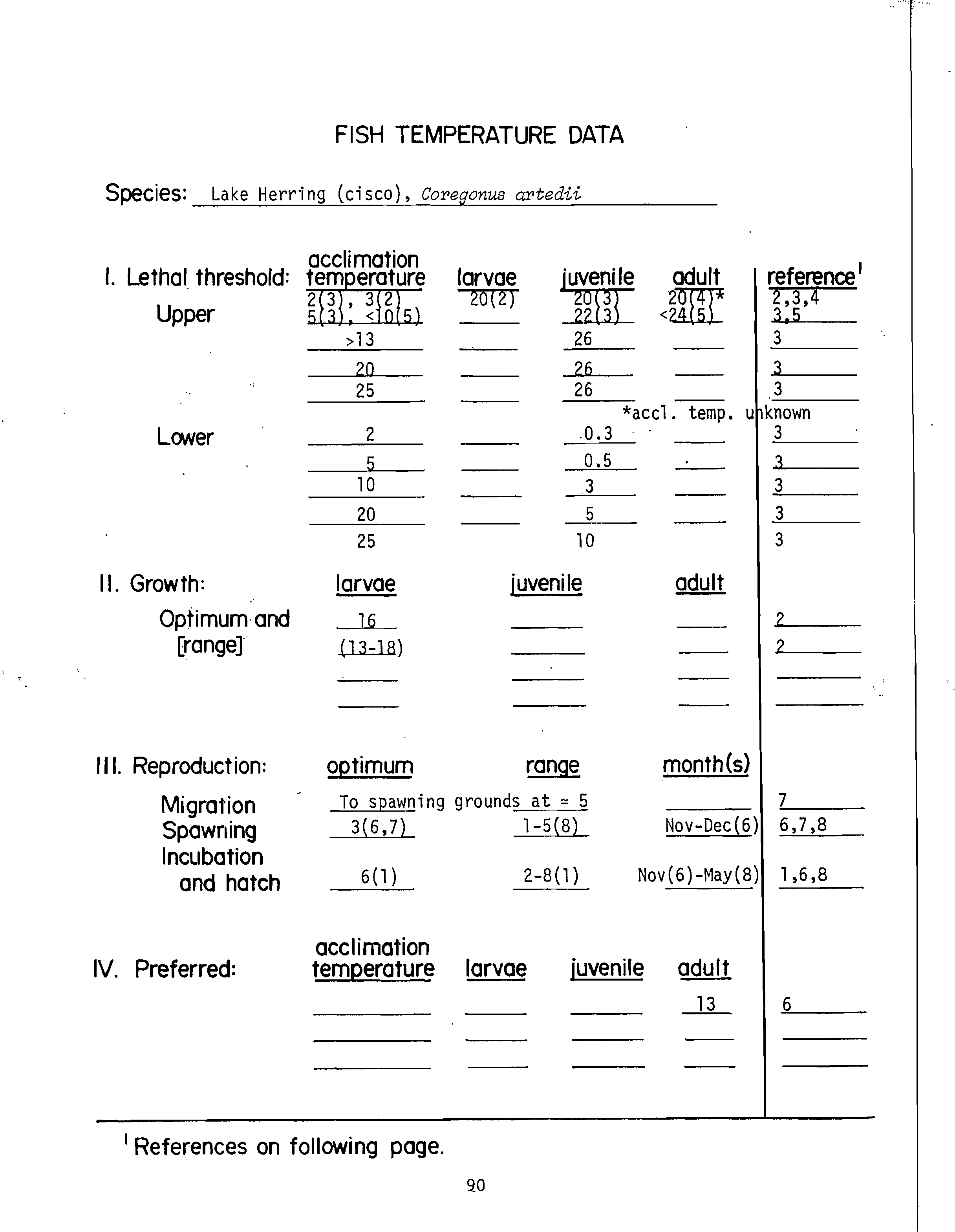
lake herring (nista)

--

17 (63)

t

25

(77)

Lake whitefish

-7

Lake trout

Largemouth bass

32 (90)

34 (93)

Northern pike

28 (82)

,

?30

(86)

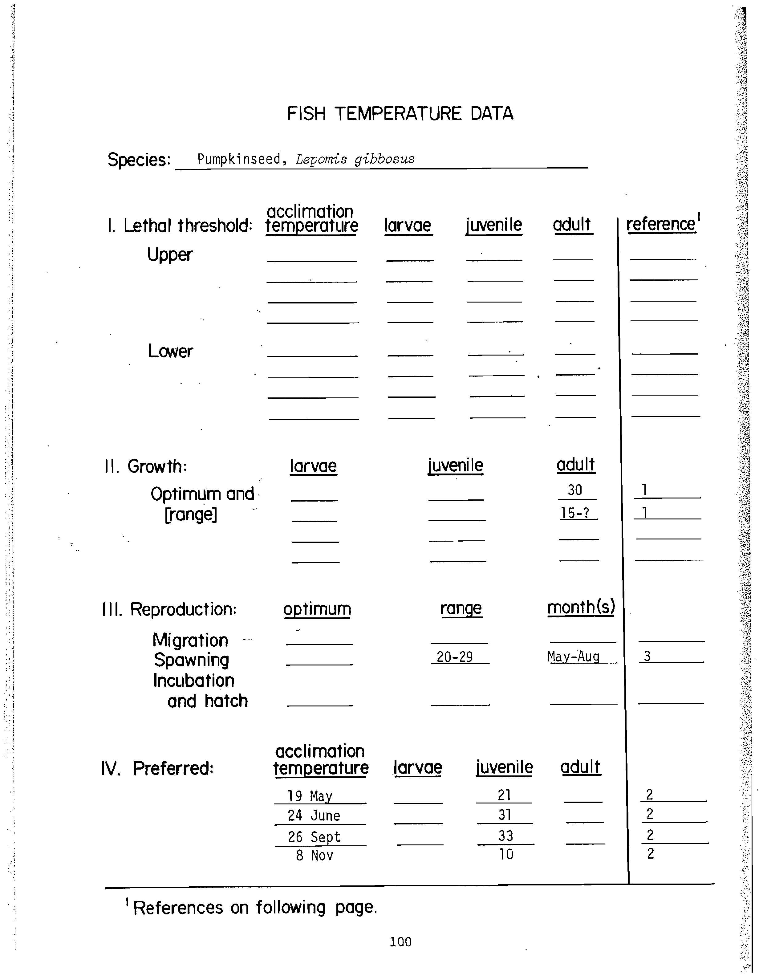
Pumpkinseed

--

Rainbow smelt

Rainbow trout

19

(66)

24 (7S)

Sauger

25

(77)

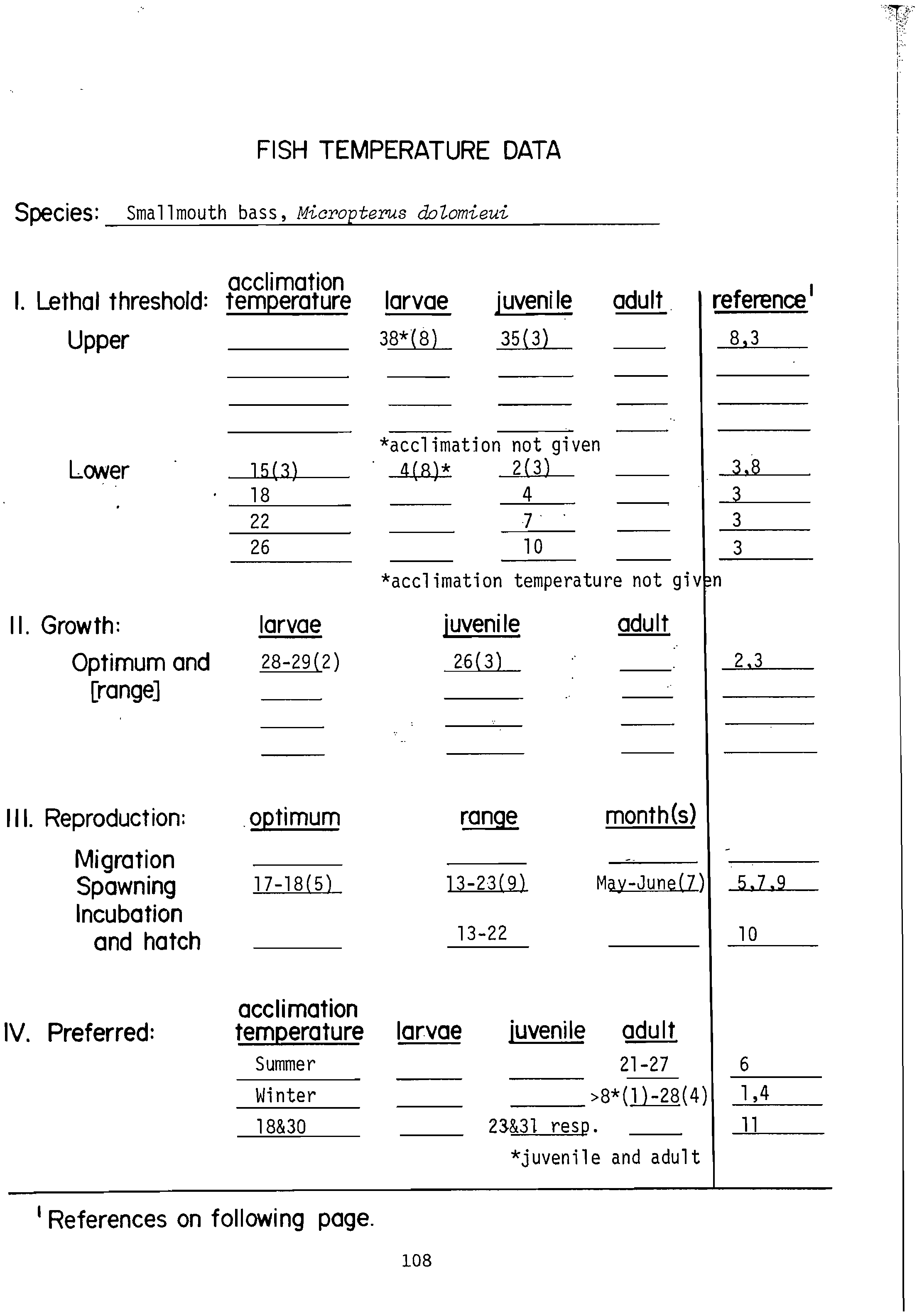
Smallmouth bass

29 (84)

Smallmouth buffalo

-

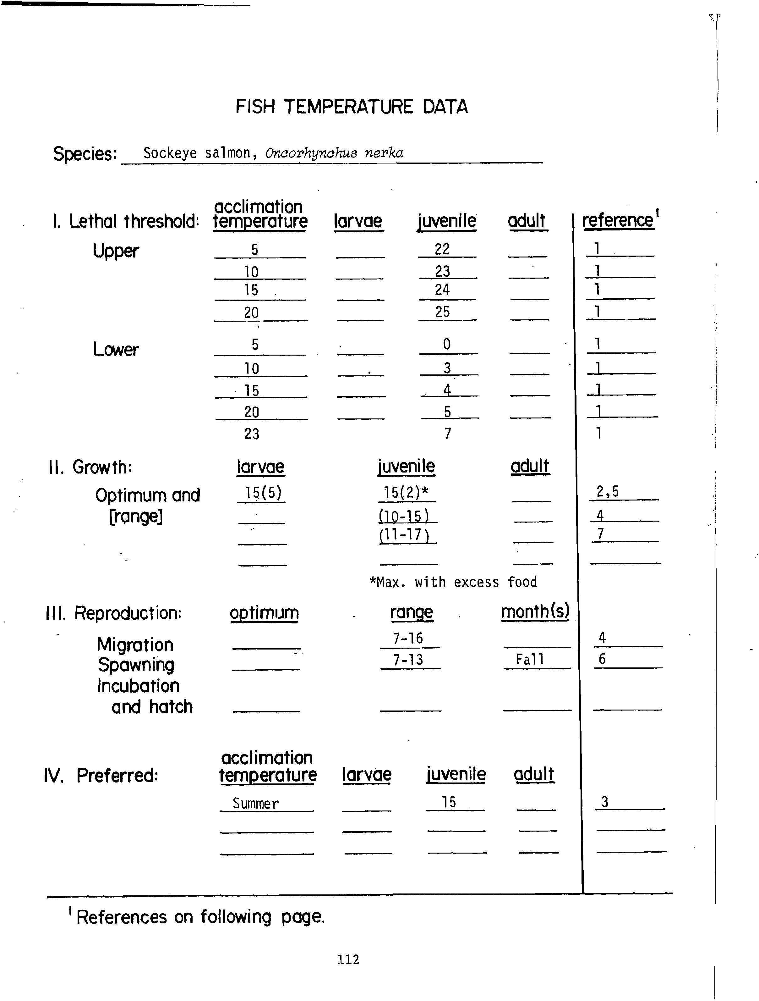
Sockeye salmon

16

(64)

22 (72)

Striped bass

Threadfin shad

Walleye

25

(77)

White bass

White crappie

28 (82)

White perch

White sucker

28 (82)t

Yellow perch

29 (84)

a

Calculated according to equation:

maximum weekly average temperature for growth optimum for growth

+ (1/3) (ultimate incipient lethal temperature - optimum for growth).

b

Based on: temperature (. C)

?

(log time (sin) - a)/b - 2

a

C, acclimation

at the maximum weekly average temperature for summer growth, and data in

Appendix B.

c

ilased on data for larvae.

14

---

SHORT-TER

M

MAXIMUM DURING GROWTH SEASON

In addition to the MWAT, maximum temperature for short exposure will

protect against potential lethal effects. We have to assume that the incipient

lethal temperature data reflecting 50 percent survival necessary for this

calculation would be based on an acclimation temperature near the MWAT for

growth. Therefore, using the data in Appendix B for the channel catfish, we

find four possible data choices near the MWAT of 32° C (again it is preferable

to use data on juveniles or adults):

Acclimation temperature

30? 32.1736

?

-0.7811

34

?

26.4204?

-0.6149

30

? 17,7125

?

-0.4058

35

?

28.3031?

-0.6554'

The formula for calculating the maximum for short exposure is:

temperature (°C) = (log time (min) - a)/b

To solve the equation we must select a maximum time limitation on this

maximum for short exposure, Since the MWAT is a weekly mean temperature

an appropriate length of time for this limitation for short exposure would

be 24 hr without risking violation of the MWAT.

Since the time is fixed at 24 hr (1,440 min), we need to solve for

temperature by using, for example, the above acclimation temperature of 30° C

for which a = 32.1736 and b = -0.7811,

temperature (° C)

log 1,440 -a

3.1584?

-32.1736

?

-29.0152

temperature

-0.7811

?

(°

-0.7811

C)

?

37,146

on solving for each of the four data points we obtain 37,1°, 37.8°, 35.9°, and

38.4° C. The average would be 37.3° C, and after subtracting the 2° C safety

factor to provide 100 percent survival, the short-term maximum for channel

catfish would be 35° C as appears in Table 1.

MAXIMUM WEEKLY AVERAGE TEMPERATURE FOR SPAWNING

From the data sheets in Apendix C one would use either the optimum

t

emperature for -spawning or, if that is_not available, the middle of the range

of

te

mperatures for spawning. Again, if

we

Use the channel catfish 'as an example,

the MWAT for spawning would be

.

27° C (Table 2). Since spawning may occur over

a period of a few weeks or months in a particular water body and only a MWAT

for

o

ptimum spawning is estimated, it would be logical to use that optimum for

the median time of the spawning season. The MWAT for the next earlier month

(° C)

a

b

15

---

TABLE 2. TEMPERATURE CRITERIA FOR SPAWNING AND EMBRYO SURVIVAL OF

SHORT EXPOSURES DURING THE SPAWNING SEASON (° C

(

0

F))

Species?

'

Maximum weekly average

temperature for spawning°

Maximum temperature for

embryo survivalb

Alewife

22?(72)

28?(82)c

Atlantic salmon

5?(41)

11?

(52)

Bigmouth buffalo

17?(63)

27?(81)c

Black crappie

17?

(63)

• 20?

(68)c

Bluegill

25?

(77)

?

•

34

?

(93)

Brook trout

9?

(48)

13?

(55)

Brown bullhead

24?(75)

27?

(81)

Brown trout

8?

(46)

15?

(59)

Carp

21'(70)

33?

(91)

Channel catfish

27?(81)

29

?

(84)c

Coho salmon

10?

(SO)

13?

(55)c

Emerald shiner

24?

(75)

28?

(82)c

Fathead minnow

24?

(75)

30?

(86)

Freshwater drum

21?

(70)

26?

(79)

Lake herring (disco)

3

?

(37)

8?(46)

Lake whitefish

5?(41)

10?

(50)c

Lake trout

9?

(48)

14?

(57)

Largemouth bass

21?

(70)

27?

(81)c

Northern pike

11?(52)

.

?19?(66)

Fumpkinieed

25?(77)

29?

(84)C

Rainbow smelt

8?(46)

15?

(59)

Rainbow trout

9?

(48)

13?

(55)

Sanger

12?

(54)

18?(64)

Smallmouth bass

17?

(63)

23?

(73)c

Smallrnouth buffalo

21?

(70)

28?

(82)c

Sockeye salmon

10?(50)

13?

(55)

Striped bass

18

?(64)

24?(75)

Throadfin shad

19

?

(66)

34?

(93)

Walleye

8?(46)

17?(63)c

White bass

17

?(63)

26?

(79)

White crappie

18?

(64)

23?

(73)

White perch

15?

(59)

20?

(66)c

White sucker

10?

(50)

20?(68)

Yellow perch

.12?

(54)

20?(68)

4

The optimum or mean of the range of spawning temperatures reported for the

species.

b The upper temperature for successful incubation and hatching reported for

the species.

c Upper temperature for spawning.

16

---

could approximate the lower temperature of the range in spawning temperature,

and the MWAT for the last month of a 3-month spawning season could approximate

the upper temperature for the range. For example, if the channel catfish

spawned from April to June the MWAT's for the 3 months would be approximately

21°, 27°, and 29° C. For fall spawning fish species the pattern or sequence

of temperatures would be reversed because of naturally declining temperatures

during their spawning season.

SHORT-TERM MAXIMUM DURING SPAWNING SEASON

If spawning season maxima could be determined in the same manner as those

for the growing season, we would be using the time-temperature equation and

the Appendix B data as before. However, growing season data are based usually

on survival of juvenile and adult individuals. Egg-incubation temperature

requirements are more restrictive (lower), and this biological process would

not be protected by maxima based on data for juvenile and adult fish. Also,

spawning itself could be prematurely stopped if those maxima were achieved.

For most species the maximum spawning temperature approximates the maximum

successful incubation temperature. Consequently, the short-term maximum

temperature should preferably be based on maximum incubation temperature for

successful embryo survival, but the maximum temperature for spawning is an

acceptable alternative. In fact, the higher of the two is probably the

preferred choice as variability in available data has shown discrepancies in

this relationship for some species.

For the channel catfish (Appendix C) the maximum reported incubation

temperature is 28° C, and the maximum reported spawning temperature is 29° C.

Therefore, the best estimate of the short-term survival of embryos would be

29° C (Table 2).-

MAXIMUM WEEKLY AVERAGE TEMPERATURE FOR WINTER

•

As discussed earlier the MWAT for winter is designed usually to prevent

fish deaths in the event the water temperature drops rapidly to an ambient

condition. Such a temperature drop could occur as the result of a power-plant

shutdown or a movement

of

the fish itself. These MWAT's are meant to apply

wherever fish can congregate, even if that is within the mixing zone.

Yellow perch require a long chill period during the winter for optimum

egg maturation and spawning (Appendix A). However, protection of this species

would be outside the mixing zone. In addition, the embryos of fall spawning

fish such as trout, salmon, and other related species such as cisco require

low incubation temperatures. For these species also the MAT during winter

would have to consider embryo survival, but again, this would be outside the

mixing zone, The mixing zone, as used in this report, is that area adjacent

to the discharge in which receiving system water quality standards do not

apply; a thermal plume therefore is not a mixing zone.

With these exceptions in mind, it is unlikely that any signficant

effects on fish populations would occur as long as death was prevented.

17

---

In many instances growth could be enhanced by controlled winter heat addition,

but inadequate food may result in poor condition of the fish.

There are fewer data for lower incipient lethal temperatures than for

the previously discussed upper incipient lethal temperatures. Appendix B

contains lower incipient lethal temperature data for only about 20 freshwater

fish species, less than half of which are listed in Tables 1 and 2. Consequent:

the available data were combined to calculate a regression line (Figure 1)

which gives a generalized MWAT for

.

winter survival instead of the species

specific approach used in the other types of criteria.

All the lower incipient lethal temperature data from Appendix C for

freshwater fish species were used to calculate the regression line, which had

a slope of 0.50 and a correlation coefficient of 0.75. This regression line

was then displaced by approximately 2.5° C since it passed through the middle

. of the data and did not represent the more sensitive species. This new line

on the edge of the data array was then displaced by a 2° C safety factor, the

same factor discussed earlier, to account for the fact that the original data

points were for 50 percent survival and the 2° C safety factor would result

in 100 percent survival, These two adjustments in the original regression

line therefore result in a line (Figure 11 that should insure no more than

negligible mortality of any fish species, At lower acclimation temperatures

the coldwater species were different from the warmwater species, and the resulta

criterion takes this into account,

If fish can congregate in an area close to-the discharge point, this

criterion could be a limit on the degree rise permissible at a particular site.

Obviously, if there is a screened discharge channel in which some cooling

occurs, a higher initial discharge temperature could be permissible to fish.

An example of the use of this criterion (as plotted in the nomograph,

Figure 1) would be a situation in which the ambient water temperature is 10°

C, and the MWAT, where fish could congregate, is 25° C, a difference of 15°

C. At a lower ambient temperature of about 2.5° C, the MWAT would be 10° C,

-a 7.5° C difference.

18

---

C:

30(86)

CC

< 25(77)

CC

LU

a

_

2

20(68)

2

a.

15(59)

—J

2

10(50)

CC

6(41)

•

0

sZ%

4./

,■.,

. P.—

WARMWATER

FISH SPECIES'

1

/

/C......... COLDWATER

/?

FISH SPECIES

/

../

I

5(41)

?

10(50)

AMBIENT TEMPERATURE

15(59)

Figure 1. Nomograph to determine the maximum weekly average

temperature of plumes for various ambient temperatures,

°C (°F).

---

SECTION 5

EXAMPLES

Again, because precise thermal-effects data are not available for all

species,• we would like to emphasize the necessity for subjective decisions

based on common-sense knowledge of existing aquatic systems. For some

fish species for which few or only relatively poor data are available,

subjectivity becomes important. If several qualified people were to calcula

various temperature criteria for species for which several sets of high qual

data were available, it is unlikely that they would be in agreement in all

instances.

The following examples for warmwater and coldwater species are presente

only as examples and are not at all intended to be water-body-specific

recommendations. Local extenuating circumstances may warrant differences,

the basic conditions of the examples may be slightly unrealistic. More

precise estimates of principal spawning and growth seasons should be

available from the local state fish departments.

EXAMPLE 1

Tables 1 and 2, Figure 1, and Appendix C are the principal data sources

for the criteria derived for this example. The following water-body-specifi

data are necessary and in this example are hypothetical:

1.

Species to be protected by the criteria: channel catfish, largemc

bass, bluegill, white crappie, freshwater drum, and bigmouth buffalo.

2.

Local spawning seasons for these species: April to June for the

white crappie and the bigmouth buffalo; other species, May to July.

3.

Normal ambient winter temperature: 5° C

in December and January;

10° C in November, February, and March.

4.

The principal growing season for these fish species: July througt

September.

5.

Any local extenuating circumstances should be incorporated into tt

criteria as appropriate. Some examples would be yellow perch gamete

maturation in the winter, very temperature-sensitive endangered species,

or important fish-food organisms that are very temperature sensitive. For

the example we will have no extenuating circumstances.

20

---

In some instances the data will be insufficient to determine each

necessary criterion for each species. Estimates must be made based on

available species-specific data or by extrapolation from data for species with

similar requirements for which adequate data are available. For instance, this

example includes the bigmouth buffalo and freshwater drum for which no growth

or short-term summer maxima are available (Table 1). One would of necessity

have to estimate that the summer criteria would not be lower than that for the

white crappie, which has a spawning requirement as low as the other two

species.

The choice of important fish species is very critical. Since in this

example the white crappie is as temperature sensitive as any of the species,

the maximum weekly average temperature for summer growth is based on the

white crappie. Consequently, this criterion would result in lower than

optimal conditions for the channel catfish, bluegill, and largemouth bass.

An alternate approach would be to develop criteria for the single most

important species even if the most sensitive is not well protected. The

choice is

. a socioeconomic one.

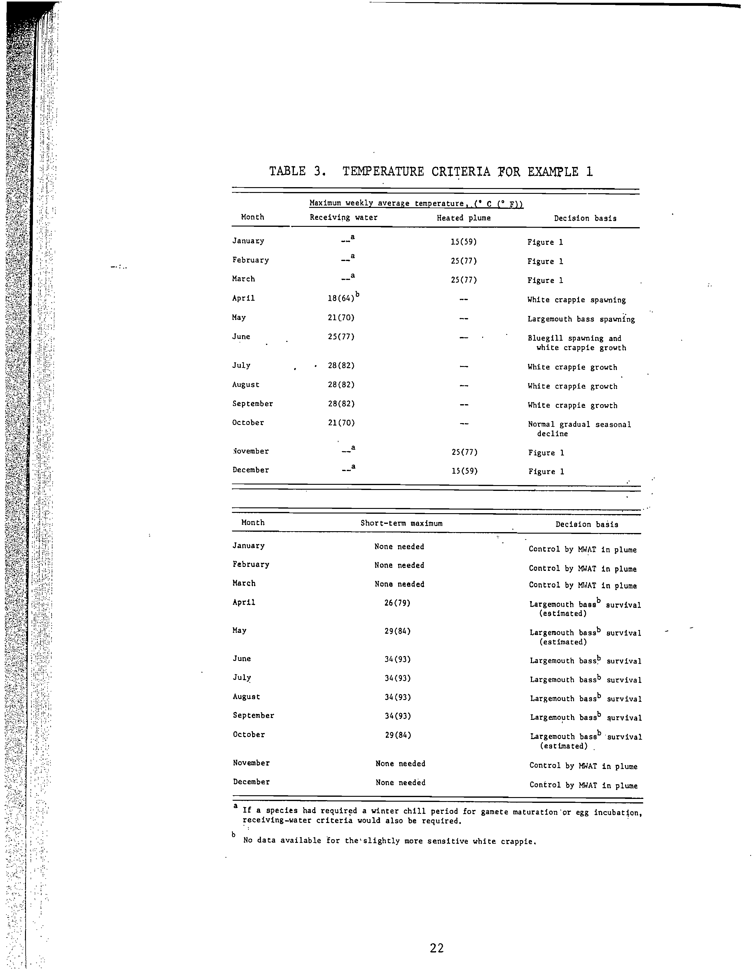
Before developing a set of criteria such as those in Table 3, the material

material in Tables 1 and 2 should be studied for the species

of concern. It is

evident that the lowest optimum temperature for summer growth for the species

for which data are available would be for the white crappie (28° C). However,

there is no maximum for short exposure since the data are not available (Appendix,

C). For the species for which there are data, the lowest maximum for short

exposure is fon:the largemouth bass-(34° C). In this example we have all

the necessary data for spawning and maximum for short exposure for embryo

survival for all species of concern (Table 2).

During the winter, criteria may be necessary both for the mixing zone as

well as for the receiving water. Receiving-water criteria would be necessary

if an important fish species were known to have gamete-maturation requirements

like the yellow perch, or embryo-incubation requirements like trout, salmon,

cisco, etc, In this example there is no need for receiving-_system water criteria.

At this point, we are ready to complete Table 3 for Example 1.

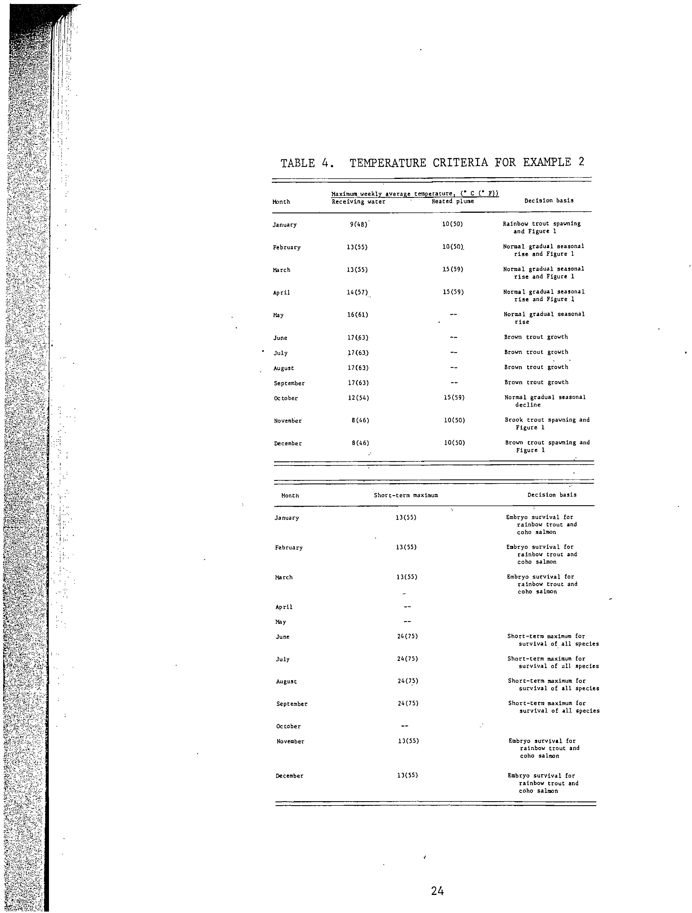
EXAMPLE 2

All of the general concerns and data sources presented throughout the

discussion and derivation of Example 1 will apply here.

1. Species to be protected by the criteria: rainbow and brown trout

and the coho salmon.

2.

Local spawning seasons for these species: November through January

for rainbow trout; and November through December

for the brown trout and coho

salmon.

3.. Normal ambient winter temperature: 2° C in November through February;

5° C in October, March, and April.

21

---

TABLE 3.?

TEMPERATURE CRITERIA FOR EXAMPLE 1

Maximum weekly average temperature,

,

•

C (° F))

Month

Receiving water

Heated plume

Decision basis

January

__ a

15(59)

Figure 1

February

--a

25(77)

Figure 1

March

25(77)

Figure 1

April

18(64)b

White crappie spawning

May

21(70)

Largemouth bass spawning

June

25(77)

Bluegill spawning and

white crappie growth

July

28(82)

White crappie growth

August

28(82)

--

White crappie growth

September

28(82)

White crappie growth

October

iovember

21(70)

a

25(77)

Normal gradual seasonal

decline

Figure 1

December

__a

15(59)

Figure 1

Month

Short—term maximum

?

Decision basis

January

?

None needed

?

Control by MWAT in plume

February

?

None needed

?

Control by MWAT in plume

March

?

Nona needed

?

Control by MWAT in plume

April?

26(79)?

Largemouth bassb

survival

(estimated)

May

?

29(84)

?

Largemouth bass

b survival

(estimated)

June

?

34(93)

?

Largemouth bass' survival

July?

34(93)

?

Largemouth bassb

survival

August

?

34(93)

?

Largemouth bass

b survival

September?

34(93)

?

Largemouth basa

l

' survival

October

?

29(84)?

Largemouth basa

l' survival

(estimated) .

November?

None needed?

Control by MWAT in plume

December

?

None needed?

Control by MWAT in plume

a

If a species had required a winter chill period for gamete maturation'or egg incubation,

receiving—water criteria would also be required.

b

No data available for the'slightly more sensitive white crappie.

22

---

4.

The principal growing season for these fish species; June through

September.

5.

Consider any local extenuating circumstances: There are none in

this example.

At this point, we are ready to complete Table 4 for Example 2.

23

---

TABLE 4.

?

TEMPERATURE CRITERIA FOR EXAMPLE 2

Month

Maximum weekly average temperature,?

(' C (" F))

Receiving water?

Heated plume

Decision basis

January

9(48)

10(50)

Rainbow trout spawning

and Figure 1

February

13(55)

10(50).

Normal gradual seasonal

rise and Figure 1

March

13(55)

15(59)

Normal gradual seasonal

rise and Figure 1

April

14(57)

15(59)

Normal gradual seasonal

rise and Figure

1

May

16(61)

Normal gradual seasonal

rise

June

17(63)

Brown trout growth

July

17(63)

Brown trout growth

August

17(63)

Brown trout growth

September

17(63)

Brown trout growth

October

12(54)

15(59)

Normal gradual seasonal

decline

November

8(46)

10(50)

Brook trout spawning and

Figure 1

December

8(46)

10(50)

Brown trout spawning and

Figure 1

Month?

Short-term maximum

?

Decision basis

January 13(55) Embryo survival for

rainbow trout and

coho salmon

February 13(55) Embryo survival for

rainbow trout and

coho salmon

March 13(55) Embryo survival for

rainbow trout and

coho salmon

April

May

June

?

24(75)?

Short-term maximum for

survival of all species

July

?

24(75)

?

Short-term maximum for

survival of all species

August?

24(75)?

Short-term maximum for

survival of all species

September?

24(75)

?

Short-term maximum for

survival of all species -

October

November 13(55) Embryo survival for

rainbow trout and

coho salmon

December 13(55) Embryo survival for

rainbow trout and

coho salmon

24

---

REFERENCES

Brett, J. R. 1952. Temperature tolerance in young Pacific salmon, genus

Oncorhynchus. J. Fish, Res. Board Can. 9:265-323,

. 1956. Some principles in the thermal requirements of fishes.

Quart. Rev. Biol, 31:75-87.

Federal Water Pollution Control Administration. National Technical Advisory

Committee. 1968. Water Quality Criteria. U.S. Department of the Interior,

Washington, D.C. 245 p.

Federal Water Pollution Control Administration. 1969a. FWPCA Presentations

ORSANCO Engineering Committee. U.S. Department of the Interior,

Sixty-Ninth Meeting, Cincinnati, Ohio (May 13-14, 19691.

. 1969b. FWPCA Presentations ORSANCO Engineering Committee.

U.S. Department of the Interior, Seventieth Meeting, Cincinnati, Ohio

(September 10, 19691.

Fry, F. E. J., J, R, Brett, arid G. 11, Clawson. 1942. Lethal limits of

temperature for young goldfish. Rev. Can, Biol. 1:50-56,

Fry, F. E. J., J. S. Hart, and K, F. Walker. 1946. Lethal temperature

relations for a sample of young speckled trout, Salvelinus fontinalis.

Ontario Fish. Res. Lab, Pub, No. 66. Univ. Toronto Press, Toronto,

Can. pp. 9-35.

Great Lakes Water Quality Agreement. 1972. With Annexes and Texts and

Terms of Reference, Between the United States of America and Canada.

TS 548;36Stat.2448. (April 15, 1972

1 . 69 p.

McKee, J; E., and H. W. Wolf, 1963, Water Quality Criteria 12nd ed.].

The Resources Agency of California Pub. No. 3-A., State Water Quality

Control Board, Sacramento, Calif. 548 p.

National Academy of Sciences and National Academy of Engineering (NAS/NAE).

1973. Water Quality Criteria 1972. A Report of the Committee on Water

Quality Criteria. U.S. Environmental Protection Agency Pub. No. EPA-R3-

73-033. Washington, D.C. 553 p.

Ohio River Valley Water Sanitation Commission (ORSANC0). Aquatic Life Advisory

Committee. 1956. Aquatic life water quality criteria ---second progress

report. Sew. Ind. Wastes 28:678-690.

25

---

. 1967, Aquatic life water quality criteria /---fourth. progress

report, Env. Sci. Tech. 1:888-897.

?

. 1970. Notice of requirements (standards number 1-70 and 2-70)

pertaining to sewage and industrial wastes discharged to the Ohio

River. ORSANCO, Cincinnati, Ohio.

Public Law 92-500. 1472. An Act to Amend the Federal Water Pollution

Control Act. 92nd Congress, S. 2770, October 18, 1972. 86 STAT. 816

through 86 STAT 904.

U.S. Environmental Protection Agency. 1976. Quality Criteria for Water.

Office of Water and Hazardous Materials, Washington, D.C. EPA 440/9-

76-023, 501 p.

26

---

APPENDICES

Page

A?

Heat. and Temperature (from the National Academy of Sciences

and National Academy of Engineering, 1973) ?

28

B

?

Thermal Tables (from the National Academy of Sciences and

'?

National Academy of Engineering, 1973).

?

51'

C?

Fish Temperature'Data (° C)

?

62

27

---

APPENDIX A*

HEAT AND TEMPERATURE

Living organisms do not respond to the quantity of heat

but to degrees of temperature or to temperature changes

caused by transfer of heat. The importance of temperature

to

acquatic organisms is well known

. , and the composition

of aquatic communities depends largely on the temperature

characteristics of their environment. Organisms have upper

and lower thermal tolerance limits, optimum temperatures

for growth, preferred temperatures in thermal gradients,

and temperature limitations for migration, spawning, and

egg incubation. Temperature also affects the physical

environment of the aquatic medium, (e.g., viscosity, degree

of ice cover, and oxygen capacity. Therefore, the com-

position of aquatic communities depends largely on tem-

perature characteristics of the environment. In recent

years there has been an accelerated demand for cooling

waters for power stations that release large quantities of

heat, causing, or 'threatening to cause, either a warming of

rivers, lakes, and coastal waters, or a rapid cooling when the

artificial sources of heat are abruptly terminated. For these

reasons, the environmental consequences of temperature

changes must be considered in assessments of water quality

requirements of aquatic organisms.

The •"natural" temperatures of surface waters of the

United States vary from 0 C to over 40 C as a function of

latitude, altitude, season, time of day, duration of flow,

depth, and many other variables. The agents that affect

the natural temperature are so numerous that it is unlikely

that two bodies of water, even in the same latitude, would

have exactly the same thermal characteristics. Moreover, a

single aquatic habitat typically does not have uniform or

consistent thermal characteristics. Since all aquatic or-

ganisms (with the exception of aquatic mammals and a

few large, fast-swimming fish) have body temperatures that

conform to the water temperature, these natural variations

create conditions that are optimum at times, but are

generally above or below optima for• particular physio-

logical, behavioral, and competitive functions of the species

present.

Because significant temperature changes may affect the

composition of an aquatic or wildlife community, an

induced change in the thermal characteristics of an eco-

system may be detrimental. On the other hand, altered

thermal characteristics may be beneficial, .as evidenced

in

most fish hatchery practices and at other aquacultural

facilities. (See the discussion of Aquaculture in Section IV.)

The general difficulty in developing suitable criteria for

temperature (which would limit the addition of heat) lies

in determining the deviation from "natural" temperature a

particular body of water can experience without suffering

adverse effects on its biota. Whatever requirements are

suggested, a "natural" seasonal cycle must be retained,

annual spring and fall changes in temperature must be

gradual, and large unnatural day-to-day fluctuations

should be avoided. In view of the many variables, it seems

obvious that no single temperature requirement can be

applied uniformly to continental or large regional areas;

the requirements must be closely related to each body of

water and to its

-

particular community of organisms,

especially the important species found in it. These should

include invertebrates, plankton, or other plant and animal

life that may be of importance to food chains or otherwise

interact with species of direct interest toman. Since thermal

requirements of various species differ, the social choice of

the species to be protected allows for different

-"levels of

protection" among water bodies as suggested by Doudoroff

and Shumway (1970)

272 for dissolved oxygen criteria. (See

Dissolved Oxygen, p. 131.) Although such decisions clearly

transcend the scientific judgments needed in establishing

thermal criteria for protecting selected species, biologists can

aid in making them. Some measures useful in assigning

levels of importance to species are: (1) high yield to com-

mercial or sport fisheries, (2) large biomass in the existing

ecosystem (if desirable), (3) important links in food chains

of other species judged important for other reasons, and

(4) "endangered" or unique status. If it is desirable to

attempt strict preservation of an existing ecosystem, the

most sensitive species or life stage may dictate the criteria

selected.

Criteria for making recommendations for water tem-

perature to protect desirable aquatic life cannot be simply a

maximum allowed change from "natural temperatures."

This is principally because a change of even one degree from

*From: National Academy of Sciences (1973), See pp. 151-171, 205-207.

---

111

152/Section III—Freshwater Aquatic Life and Wildlife

an ambient temperature has varying significance for an

organism, depending upon where the ambient level lies

within the tolerance range. In addition, historic tempera-

ture records or, alternatively, the existing ambient tempera-

ture prior to any thermal alterations by man are not always

reliable indicators of desirable conditions for aquatic

populations. Multiple developments of water resources also

change water temperatures both upward (e.g., upstream

power plants or shallow reservoirs) and downward (e.g.,

deepwater releases from large reservoirs), so that "ambient"

and "natural" are exceedingly difficult to define at a given

point over periods of several years.

Criteria for temperature should consider both the multiple

thermal requirements of aquatic species and requirements

for balanced communities. The number of distance require-

ments and the necessary values for each require periodic

reexamination as knowledge of thermal effects on aquatic

species and communities increases. Currently definable

requirements include:

•

maximum sustained temperatures that are con-

sistent with maintaining desirable levels of pro-

ductivity;

•

maximum levels of metabolic acclimation to warm

temperatures that will permit return to ambient

winter temperatures should artificial sources of

heat cease;

•

temperature limitations for survival of brief exposures

to temperature extrenies, both upper and lower;

• restricted temperature ranges for various stages of

reproduction, including (for fish) gonad growth and

gamete maturation, spawning migration, release of

gametes, development of the embryo, commence-

ment of independent feeding (and other activities)

by juveniles; and temperatures required for meta-

morphosis, emergence, and other activities of lower

forms;

•

thermal limits for diverse compositions of species of

aquatic communities, particularly where reduction

in diversity creates nuisance growths of certain

organisms, or where important food sources or

chains are altered ;

•

thermal requirements of downstream aquatic life

where upstream warming of a cold-water source will

adversely affect downstream temperature require-

ments.

Thermal criteria must also be formulated with knowledge

of how man alters temperatures, the hydrodynamics of the

c

hanges, and how the biota can reasonably be expected to

interact with the thermal regimes produced. It is not

su

fficient, for example, to define only the thermal criteria

for sustained production of a species in open waters, because

large numbers of organisms may also be exposed to thermal

c

hanges by being pumped through the condensers and

mixing zone of a power plant. Design engineers need

29

particularly to know the biological limitations to their

design options in such instances. Such considerations may

reveal nonthermal impacts of cooling processes that may

outweigh temperature effects, such as impingement of fish

upon intake screens, mechanical or chemical damage to

zooplankton in condensers, or effects of altered current

patterns on bottom fauna in a discharge area. The environ-

mental situations of aquatic organisms (e.g., where they

are, when they are there, in what numbers) must also be

understood. Thermal criteria for migratory species should

be applied to a certain area only when the species is actually

there. Although thermal effects of power stations are

currently of great interest, other less dramatic causes of

temperature change including deforestation, stream chan-

nelization, and impoundment of flowing water must be

recognized.

DEVELOPMENT OF CRITERIA

Thermal criteria necessary for the protection of species or

communities are discussed separately below. The order of

presentation of the different criteria does not imply priority

for any one body of water. The descriptions define preferred

methods and procedures for judging thermal requirements,

and generally do not give numerical values (except in

Appendix II–C). Specific values for all limitations would

require a biological handbook that is far beyond the scope

of this Section. The criteria may seem complex, but they

represent an extensively developed framework of knowledge

about biological responses. (A sample application of these

criteria begins on page 166, Use of Temperature Criteria.)

TERMINOLOGY DEFINED

Some basic thermal responses of aquatic organisms will

be referred to repeatedly and are defined and reviewed

briefly here. Effects of heat on organisms and aquatic

communities have been reviewed periodically (e.g., Bullock

1955,

259 Brett 1956;2 " Fry 1947,

276

1964,

276

1967;2

" Kinne

1970

29

9. Some effects have been analyzed in the context of

thermal modification by power plants (Parker and Krenkel

1969; 308

Krenkel and Parker 1969;

298

Cairns 1968;

261 Clark

1969;

263

and Coutant 1970c

269

). Bibliographic information

is available from Kennedy and Mihursky (1967),

294

Raney

and Menzel (1969), 313 and from annual reviews published

by the Water Pollution Control Federation (Coutant

1968,2"

1969,

266 1970a,262

197 1270).

Each species (and often each distinct life-stage of a species)

has a characteristic tolerance range of temperature as a

consequence of acclimations (internal biochemical adjust-

ments) made while at previous holding temperature (Figure

111-2; Brett 1956

253

). Ordinarily, the ends of this range, or

the lethal thresholds, are defined by survival of 50 per cent

of a sample of individuals. Lethal thresholds typically are

referred to as "incipient lethal temperatures," and tem-

perature beyond these ranges would be considered "ex-

---

Ultimate incipient lethal temperature

25 —

lethal threshold 50%

lethal threshold 5%

r

?

loading

(activity

level

growth)

28

24

22

Heat and Temperature/153

treme." The tolerance range is adjusted upward by ac-

climation to warmer water and downward to cooler water,

although there is a limit to such accommodation. The

lower end of the range usually is at zero degrees centigrade

(32 F) for species in temperate latitudes (somewhat less for

saline waters), while the upper end terminates in an

"ultimate incipient lethal temperature" (Fry et al. 1946281).

This ultimate threshold temperature represents the "break-

ing point" between the highest temperatures to which an

animal can be acclimated and the lowest of the extreme

temperatures that will kill the warm-acclimated organism.

Any rate of temperature change over a period of minutes

5

Acclimation temperature—Centigrade

10?

100?1,000

Time to 50% mortality—Minutes

10,000

After Brett 1952

252

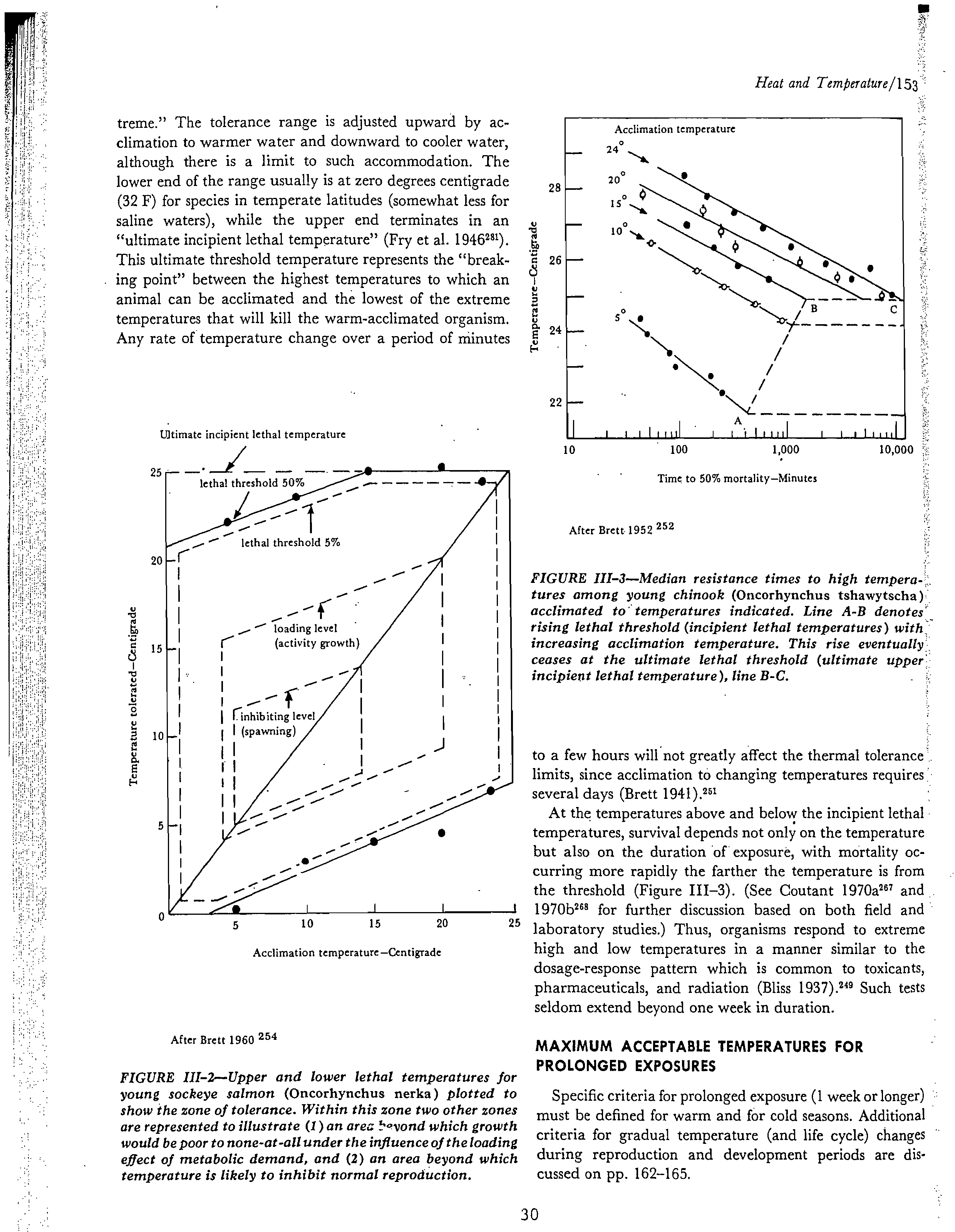
FIGURE III-3—Median resistance times to high tempera-

tures among

young

chinook

(Oncorhynchus tshawytscha)

acclimated to temperatures indicated. Line A-B denotes' _

rising lethal threshold (incipient lethal temperatures) with:

increasing acclimation temperature. This rise eventually

ceases at the ultimate lethal threshold (ultimate

upper

incipient lethal temperature), line B-C.

to a few hours will not greatly affect the thermal tolerance

limits, since acclimation to changing temperatures requires

several days (Brett 1941).2"

At the temperatures above and below the incipient lethal

temperatures, survival depends not only on the temperature

but also on the duration of exposure, with mortality oc-

curring more rapidly the farther the temperature is from

the threshold (Figure 111-3). (See Coutant 1970a

267 and

•

? I?

I

?

1970b2" for further discussion based on both field and

10?

15

?

20?

25

laboratory studies.) Thus, organisms respond to extreme

high and low temperatures in a manner similar to the

dosage-response pattern which is common to toxicants,

pharmaceuticals, and radiation (Bliss 1937). 2 " Such tests

seldom extend beyond one week in duration.

After Brett 1960 254

FIGURE III-2—Upper and lower lethal temperatures for

young

sockeye

salmon

(Oncorhynchus nerka)

plotted to

show the

zone

of tolerance. Within this zone two other zones

are represented to illustrate (1)

an

area !

•o

vond which growth

would be poor to none-at-all under the influence of the loading

effect of metabolic demand, and

(2) an

area beyond which

temperature is likely to inhibit normal reproduction.

MAXIMUM ACCEPTABLE TEMPERATURES FOR

PROLONGED EXPOSURES

Specific criteria for prolonged exposure (1 week or longer)

must be defined for warm and for cold seasons. Additional

criteria for gradual temperature (and life cycle) changes

during reproduction and development periods are dis-

cussed on pp. 162-165.

30

---

),0

00

pera-s.:

;cha)::

with

ually

ire

/

15

3

?

154 /Section 111—Freshwater Aquatic Life and Wildlife

SPRING, SUMMER, AND FALL MAXIMA FOR

PROLONGED EXPOSURE

ince

tires ..1'

thal

r7.

ture

OC-

70M

and

and

:me

the

nts,

ests

er

g

aal -

;es

fis-

Occupancy of habitats by most aquatic organisms is

often limited within the thermal tolerance range to tem-

peratures somewhat below the ultimate upper incipient

lethal temperature. This is the result of poor physiological

performanc

e

at near lethal levels (e.g., growth, metabolic

scope for activities, appetite, _food conversion efficiency),

.interspecies competition, disease, predation, and other

subtle ecological factors (Fry 1951;

2

" Brett 1971

25

9. This

complex limitation is evidenced by restricted southern and

altitudinal distributions of many species. On the other hand,

optimum temperatures (such as those producing fastest

growth rates) are not generally necessary at all times to

maintain thriving populations and are often exceeded in

nature during 'summer months (Fry 1951;

2

" Cooper 1953;2"

Beyerle and Cooper 1960;

246

Kramer and Smith 1960207).

Moderate temperature fluctuations can generally • be

tolerated as long as a maximum upper limit is not exceeded

for long periods.

A true temperature limit for exposures long enough to

reflect metabolic acclimation and optimum ecological per-

formance must lie somewhere between the physiological

optimum and the ultimate upper incipient lethal tempera-

tures. Brett (1960)

2

" suggested that a provisional long-

term exposure limit be the temperature greater than opti-

mum that allowed 75 per cent of optimum performance.

His suggestion has not been tested by definitive studies.

Examination of literature on performance, metabolic

rate, temperature preference, growth, natural distribution,

and tolerance of several species has yielded an apparently

sound theoretical basis for estimating an upper temperature

limit for long term exposure and a method for doing this

with a minimum of additional research. New data will

provide refinement, but this method forms a useful guide

for the present time. The method is based on the general

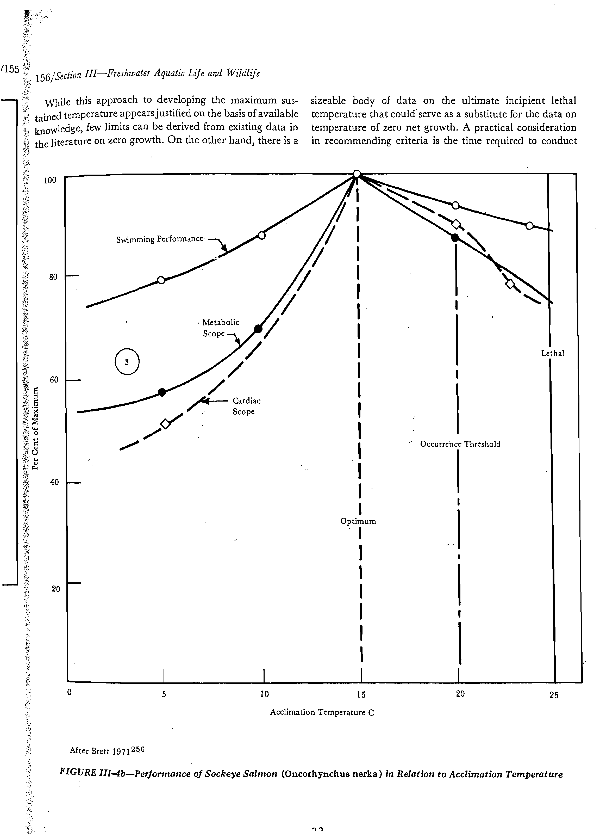
observations summarized here and in Figure III-4(a, b, c).

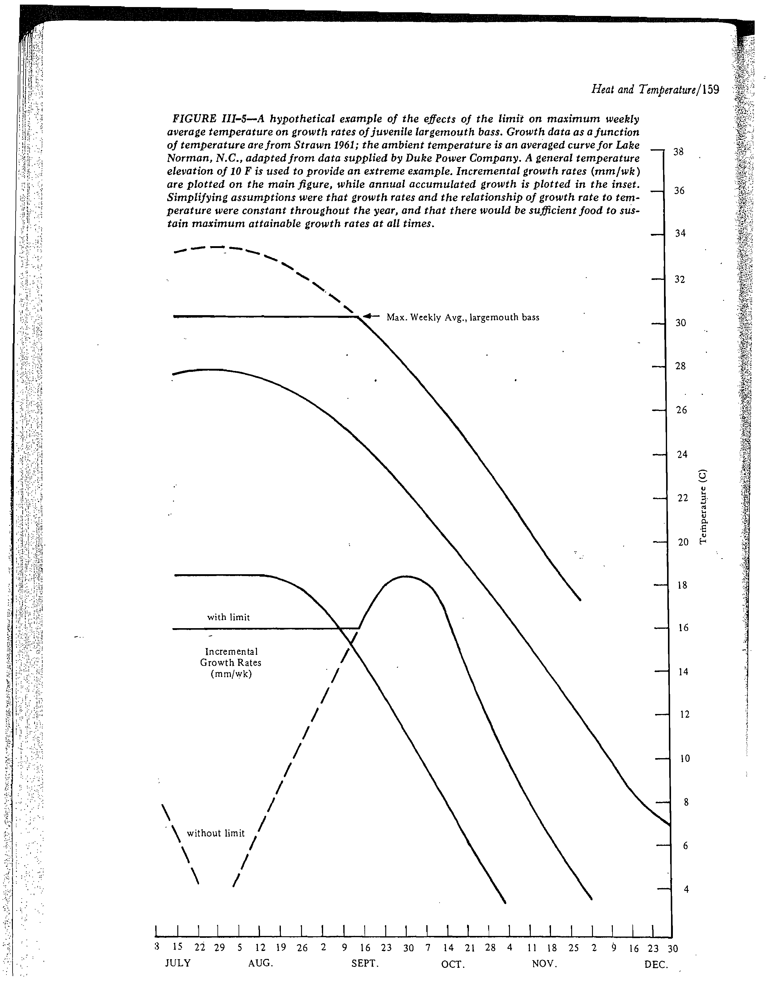
1.

Performances of organisms over a range of tempera-

tures are available in the scientific literature for a variety of

functions. Figures III-4a and b show three characteristic

types of responses numbered 1 through 3, of which types 1

and 2 have coinciding optimum peaks. These optimum

temperatures are characteristic for a species (or life stage).

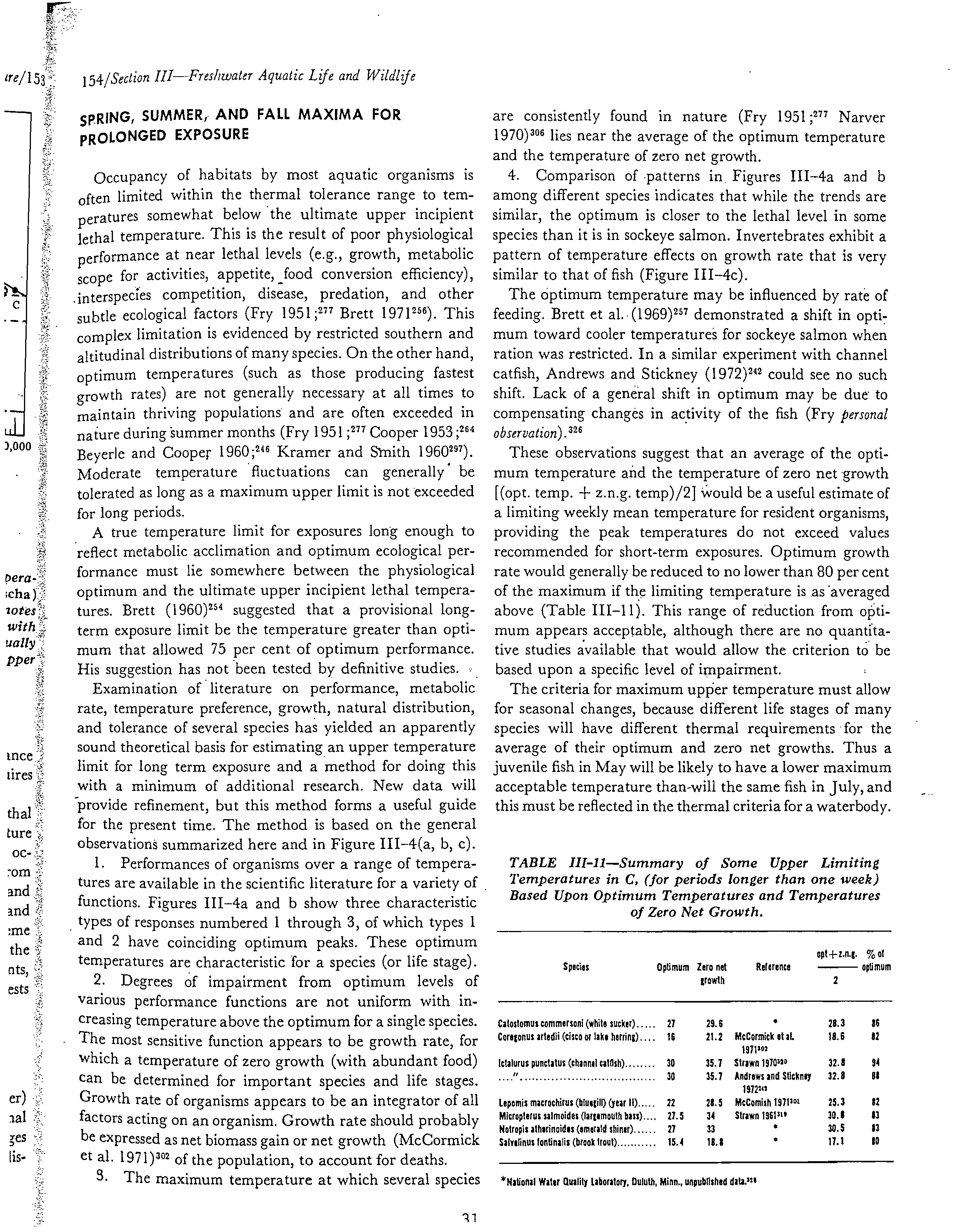
2.

Degrees of impairment from optimum levels of

various performance functions are not uniform with in-

creasing temperature above the optimum for a single species.

The most sensitive function appears to be growth rate, for

which a temperature of zero growth (with abundant food)

can be determined for important species and life stages.

Growth rate of organisms appears to be an integrator of all

factors acting on an organism. Growth rate should probably

be expressed as net biomass gain or net growth (McCormick

et al. 1971)

302

of the population, to account for deaths.

S. The maximum temperature at which several species

are consistently found in nature (Fry 1951;

2

" Narver

1970)

306

lies near the average of the optimum temperature

and the temperature of zero net growth.

4. Comparison of patterns in

.

Figures III-4a and b

among different species indicates that while the trends are

similar, the optimum is closer to the lethal level in some

species than it is in sockeye salmon. Invertebrates exhibit a

pattern of temperature effects on growth rate that is very

similar to that of fish (Figure III-4c).

The optimum temperature may be influenced by rate of

feeding. Brett et al. (1969)

257

demonstrated a shift in opti-

mum toward cooler temperatures for sockeye salmon when

ration was restricted. In a similar experiment with channel

catfish, Andrews and Stickney (1972)

2

" could see no such

shift. Lack of a general shift in optimum may be due to

compensating changes in activity of the fish (Fry

personal

observation). 326

These observations suggest that an average of the opti-

mum temperature and the temperature of zero net growth

[(opt. temp. + z.n.g. temp)/2J Would be a useful estimate of

a limiting weekly mean temperature for resident organisms,

providing the peak temperatures do not exceed values

recommended for short-term exposures. Optimum growth

rate would generally be reduced to no lower than 80 per cent

of the maximum if the limiting temperature is as 'averaged

above (Table III-11). This range of reduction from opti-

mum appears acceptable, although there are no quantita-

tive studies available that would allow the criterion to be

based upon a specific level of impairment.

The criteria for maximum upper temperature must allow

for seasonal changes, because different life stages of many

species will have different thermal requirements for the

average of their optimum and zero net growths. Thus a

juvenile fish in May will be likely to have a lower maximum

acceptable temperature than-will the same fish in July, and

this must be reflected in the thermal criteria for a waterbody.

TABLE 111-11—Summary of Some Upper Limiting

Temperatures

in C,

(f

or

periods longer

than one

week)

Based Upon

Optimum

Temperatures and Temperatures

of Zero Net Growth.

Species

Optimum?Zero net

growth

Reference

opt+z.n.g. % of

optimum

2

Catostomus commersoni (white sucker) ?21

29.6

•

28.3

86

Coregonus artedli (circa or lake herring).

? 16

21.2

McCormick et al.

18.6

82

1971"

Ictalurus punctatus (channel cash) ?30

35.7

Straws 1970

31

0

32.8

94

30

35.1

Andrews and Stickney

32.8

81

1972"

Lepomis macrochirus (bluegill) (year II)

?22

28.5

McComish 1971

501

25.3

82

Micropterus salmoides (largemouth bass) ?

21.5

34

Strewn 1951"

30.1

13

Notropis atherinoidss (emerald shiner)

?27

33

•

30.5

13

Saly

elinus tontinalis (brook trout) ?

15.4

18.8

•

17.1

10

*National Water Quality Laboratory, Duluth, Minn., unpublished data."

'1

1

---

100

Gross Conversion Efficiency,

90

Lethal

80

70

Digestion Rate

60

50

Occurrence Threshold

40

30

Growth Rate

Opt mum

20

10

Heat and Temperature/155

0

10

15

Acclimation Temperature C

20

?

25

After Brett 1971256

Maximum Meal Size

FIGURE III-la—Performance of Sockeye Salmon

(Oncorhynchus nerka) in

Relation

to

Acclimation Temperature

32

---

Swimming Performance

• Metabolic

Scope

Cardiac

Scope

/

I

°

Optimum

1

Lethal

Occurrence Threshold

156/Section III—Freshwater Aquatic Life and Wildlife

While this approach to developing the maximum sus-

tained temperature appears justified on the basis of available

knowledge, few limits can be derived from existing data in

the literature on zero growth. On the other hand, there is a

sizeable body of data on the ultimate incipient lethal

temperature that could serve as a substitute for the data on

temperature of zero net growth. A practical consideration

in recommending criteria is the time required to conduct

/155

100

80

60

20

0

5

10

15

20

25

Acclimation Temperature C

After Brett 1971256

FIGURE III-4b—Performance of Sockeye Salmon

(Oncorhynchus nerka) in

Relation to Acclimation Temperature

---

0

200

150 -

00

f33

et

•

00

0 0%

0

#

1

0.0

•

o

o

0.1?

0

•

0

fioo

0

?

e

90

er°

8

o?

0

0 0

c

0

g

?

• o

o

0 •

o

%.

•0 a•

O1

°

o

k arm iiiissi 1 i eel

9?

5

10

15

20

25

Temperature in C

0

o

0

50

0

Heat and Temperature/157

research necessary to provide missing data. Techniques for

determining incipient lethal temperatures are standardized

(Brett 1952)

2" whereas those for zero growth are not.

A temperature that is one-third of the range between the

optimum temperature and the ultimate incipient lethal

temperature that can be calculated by the formula

ultimate incipient lethal temp.-optimum temp.

optimum temp. + ?

3

(Equation 1)

yields values that are very close to (optimum temp. +

z.n.g. temp.)/2. For example, the values are, respectively,

32.7 and 32.8 C for channel catfish and 30.6 and 30.8 for

largemouth bass (data from Table 111-8 and Appendix

. II).

This formula offers a practical method for obtaining allow- .

Ansell 1968

243

FIGURE III-4c—M.

mercenaria:

The general relationship

between temperature and the rate of shell growth, based

on

field measurements of growth and temperature.

sites in Poole Harbor, England; 0: North American sites.

able limits, while retaining as its scientific basis the require-

ments of preserving adequate rates of growth. Some limits

obtained from data in the literature are given in Table

111-12. A hypothetical example of the effect of this limit on

growth of largemouth bass is illustrated in Figure 111-5.

Figure 111-5 shows a hypothetical example of the effects

of the limit on maximum weekly average temperature on

growth rates of juvenile largemouth, bass. Growth data as a

function of temperature are from Strawn 1961 319

; the ambi-

ent temperature is an averaged curve for Lake Norman,

N. C., adapted from data supplied by Duke Power Com-

pany. A general temperature elevation of 10 F is used to

provide an extreme example. Incremental growth rates

(mm/wk) are plotted on the main figure, while annual ac-

cumulated growth is plotted in the inset. Simplifying as- '

sumptions were that growth rates and the relationship of '

growth rate to temperature were constant throughout the

year, and that there would be sufficient food to sustain

maximum attainable growth rates at all times.

The criterion for a specific location would be determined

by the most sensitive life stage of, an important species

likely to be present in that location at that time. Since

many fishes have restricted habitats (e.g., specific depth

zones) at many life stages, the thermal criterion must be

applied to the proper zone. There is field evidence that fish

avoid localized areas of unfavorably, warm water. This has

been demonstrated both in lakes where Coldwater fish

normally evacuate warm shallows in summer (Smith

1964) 3 '8

and at power station mixing zones (Gammon

1970;2 " Merriman et al. 1965).

304

In most large bodies of

water there are both vertical and horizontal thermal

gradients -that mobile organisms can follow to avoid un-

favorable high (or low) temperatures.

The summer maxima need not, therefore, apply to

mixing zones that occupy a small percentage of the suitable

habitat or necessarily to all zones where organisms have

free egress to cooler water. The maxima must apply, how-

ever, to restricted local habitats, such as lake hypolimnia or

thermoclines, that provide important summer sanctuary

areas for cold-water species. Any avoidance of a warm area

not part of the normal seasonal habitat of the species will

mean that less area of the water body is available to support

the population and that production may be reduced. Such

reduction should not interfere with biological communities

or populations of important species to a degree that is

damaging to the ecosystem or other beneficial uses. Non-

mobile organisms that must remain in the warm zone will

probably be the limiting organisms for that location. Any

recommendation for upper limiting temperatures must be

applied carefully with understanding of the population

dynamics of the species in question in order to establish

both local and regional requirements.

---

Elevated (with limit)

Elevated (without limit)

Average Ambient.,

(Lake Norman, N.C.)

Weekly Growth Rate

(Ambient + 10 F)

Weekly Growth Rate

(Ambient)

Ambient + 10 F

158 I Section III—Freshwater Aquatic Life and Wildlife

Annual Accumulated Growth

250

6 200

-5

150

60

U

50

2?

4?

6?

8?

10?

12

Weeks

6

3

•

2 5

4

10

9

8

7

2

3

i?

I

?

I

?

I?

I?

I?

I

?

I?

I?

I?

I?

I?

I

?

i

?

l?

I?

I?

I?

I?

I?

I?

I?

I?

I

?0?

7 14 21?

28 4 11 18?

25 4?

11 18 25

?

1

?

8 15 22 29 6

?

13 20 27 3 10 17 24 1

JAN.

?

FEB.

?

MAR.?

APR.

?

MAY

?

JUNE

35

---

U

U

22

20

18

16

14

12

10

8

6

4

Heat and Temperature/ 159

FIGURE III-5—A hypothetical example of the effects of the limit

on maximum

weekly

average temperature on growth rates of juvenile

largemouth

bass. Growth

data

as a function

of temperature are from Strawn 1961; the ambient temperature is

an

averaged curve for Lake

Norman, N.C., adapted from data supplied by Duke Power

Company. A

general temperature

elevation of 10 F is used to provide

an

extreme example. Incremental growth rates (mm/wk)

are plotted on the main figure, while annual accumulated growth is plotted in the inset.

Simplifying assumptions were that growth rates and the relationship of growth rate to

tem-

perature

were constant throughout the year, and that there would be sufficient food to sus-

tain maximum attainable growth rates at all times.

'0— Max. Weekly Avg., largemouth bass

••••■•■1

111111111111111_1111111111

3

15

22

29

5 12 19 26 2

9 16 23 30

7 14 21 28 4

11

18 25 2

9 16 23 30

JULY

AUG.

SEPT.

OCT.

NOV.

DEC.

with limit

Incremental

Growth Rates

(mm/wk)

I

without limit /

/

38

36

34

32

30

28

26

24

---

Micropterus dolomitic (smallmouth bass)._

Micropterussalmoides (largemouth bass)(try).

21.5

Notropis atherinoides (emerald shiner) .....

21

Oncorhynchus nerka (sockeye salmon)

?

15.0

15.0

(juveniles)

?

15.0

Pseudopleuronectes Americanus (winter

flounder)

?

18.0

Sams

truth (brown trout)

?

Ito 11

ave 12.5

Salvelinus footinalis (brook trout)

?

Salvolinus namaycush (lake trout) ?

26.3

?

83?

growth

28.3?

83

?

• growth

ave 21.3?

81.1

11.5?

growth

80.6?

growth

59.0?

growth

59.0•

?

other functions

max. swimming

64.4?

growtt7

54.5?

growth

15.4

?

59.1

?

growth

13.0?

55.4

?

growth

15?

59?

metabolic

ave 14.5?

53.1?

scope

16?

60.8?

scope tor activity

(2 metabolism)

17?

62.6

?

swimming speed

ave 16.5?

61.1

160/Section III-Freshwater Aquatic Life and Wildlife

TABLE m-12-Summary of Some Upper Limiting Temperatures for Prolonged Exposures of Fishes Based on

Optimum Tem-

peratures

and Ultimate Upper Incipient Lethal Temperatures (Equation 1).

Reference

Ultimate upper incipient

lethal temperature

C

Reference

Maximum weekly average

temperature (Eq. 1)

C?

F

unpubl., NWC11.324

29.3

84.1

Hart 1941"

21.8

82

McCormick

et

a1.1971'02

25.1

71.3

Edsall and Colby 19102

2

4

19.2

66.6

Straws 1970;

420

Andrews and Stickney

38.0

100.4

Allen and Strewn 1961

140

32.1

90.9

1911242

McComish 1971"

33.8

92.8

Hart 19522

44

25.9

11.6

Anderson 1959241

Horning and Pearson 1972291

35.0

95.0

Horning and Pearson 1912

241

29.9

85.8

Peek 196520

Strewn 196149

36.4

91.5

Hera 1952446

30.5

86.7

unpubL, NWEI1.321

30.1

81.3

Hart 1952244

21.2

82.1

Brett et a1.1969257

25.0

71.0

Brett 1952242

18.3

64.9

Brett 1971244

Brett 1970244

29.1

84.4

HMI and Westman 1966"

21.1

11.2

Brett 1910245

23.5

74.3

Bishai 1960247

16.2

61.2

unpubl, NWOL42s

25.5

11.9

Fry, Hart

and

Walker, 1946241

11.2

64.8

Baldwin 1951244

Graham 1949444

Gibson and Fry 1954"

23.5

Gibson and Fry 1954

213

18.8

65.8

Optimum

Species

?

Function

C?

F

Catostomus commersoni (white sucker)

??

27?

80.6

?

growth

Coregonus artedli (Cisco or rake herring) •

?

16?

60.1?

growth

Ictaluros punctatus (channel catfish)

??

30

?

86?

growth

Lepomis macrochiros (bluegill) (yr 11)

??

22?

71.6?

growth

Heat added to upper reaches of some cold rivers can be

retained throughout the river's remaining length ( Jaske

and Synoground 1970).

292

This factor adds to the natural

trend of warming at distances from headwaters. Thermal

additions in headwaters, therefore, may contribute sub-

stantially to reduction of cold-water species in downstream

areas (Mount 1970).

3

" Upstream thermal additions should

be evaluated for their effects on summer maxima at down-

stream locations, as well as in the immediate vicinity of

the heat source.

Recommendation

Growth of aquatic

organisms would be main-

tained at levels necessary for sustaining actively

growing and reproducing populations if

the maxi-

mum weekly average temperature in the zone in-

habited by the species

at that time does not exceed

o

ne-third of the range between the optimum tem-

p

erature and the ultimate upper incipient lethal

te

mperature of the species (Equation

1,

page 157),

and the temperatures above the weekly average do

not exceed the criterion for

short-term exposures.

This maximum need

not apply to

acceptable mix-

ing zones (see proportional relationships of mixing

zones to receiving systems, p. 114), and must be

ap

se

asonal

plied with

distribution

adequate

of

understanding

the important

of

species.

the normal

WINTER MAXIMA

Although artificially produced temperature elevations

during winter months may actually bring the temperature

closer to optimum or preferred temperature for important

species and attract fish (Trembley 1965),

3

" metabolic

acclimation to these higher levels can preclude safe return

of the organism to ambient temperatures should the

artificial heating suddenly cease (Pennsylvania Fish Com-

mission 1971;

2

" Robinson 1970)

3

" or the organism be

driven from the heat area. For example, sockeye salmon

(Oncorhynchus nerka)

acclimated to 20 C suffered 50 percent

mortality in the laboratory when their temperature was

dropped suddenly to 5 C (Brett 1971:

2

" see Figure

111-3).

The same population of fish withstood a drop to zero when

acclimated to 5 C. The lower limit of the range of thermal

tolerance of important species must, therefore, be main-

tained at the normal seasonal ambient temperatures

throughout cold seasons, unless special provisions are made

to assure that rapid temperature drop will not occur or that

organisms cannot become acclimated to elevated tempera-

tures. This can be accomplished by limitations on tempera-

ture elevations in such areas as discharge canals and mixing

zones where organisms may reside, or by insuring that

maximum temperatures occur only in areas not accessible

to important aquatic life for lengths of time sufficient to

allow metabolic acclimation. Such inaccessible areas would

include the high-velocity zones of diffusers or screened

---

Heat and Temperature/ 161

charge channels. This reduction of maximum temperatures

would not preclude use of slightly warmed areas as sites for

intense winter fisheries.

This consideration may be important in some regions at

times other than in winter. The Great Lakes, for example,

are susceptible to rapid changes in elevation of the thermo-

cline in summer which may induce rapid decreases in

shoreline temperatures. Fish acclimated to exceptionally

high temperatures in discharge canals may be killed or

severely stressed without changes in power plant opera-

tions (Robinson 1968). 3 " Such regions should take special

note of this possibility.

Some numerical values for acclimation temperatures and

lower limits of tolerance ranges (lower incipient lethal

temperatures) are given in Appendix II–C. Other data must

be provided by further research. There are no adequate

data available with which to estimate a safety factor for no

stress from cold shocks. Experiments currently in progress,

however, suggest that channel catfish fingerlings are more

Susceptible to predation after being cooled more than 5 to

6 C (Coutant,

unpublished data).324

The effects of limiting ice formation in lakes and rivers

should be carefully observed. This aspect of maximum

winter temperatures is apparent, although there is insuffi-

cient evidence to estimate its importance.

Recommendation

Important species should be protected if the

maximum weekly average temperature during win-

ter months in any area to which they have access

does not exceed the acclimation temperature

(minus a 2 C safety factor) that raises the lower

lethal threshold temperature of such species above

the normal ambient water temperatures for that

season, and the criterion for short-term exposures

is not exceeded. This recommendation applies es-

pecially to locations where organisms may be at-

tracted from the receiving water and subjected to

rapid thermal drop, as in the low velocity areas of

water diversions (intake or discharge), canals, and

mixing zones.

SHORT-TERM EXPOSURE TO EXTREME TEMPERATURE

To protect aquatic life and yet allow other uses of the

water, it is essential to know the lengths of time organisms

can survive extreme temperatures (i.e., temperatures that

exceed the 7-day incipient lethal temperature). Both

natural environments and power plant cooling systems can

briefly reach temperature extremes (both upper and lower)

without apparent detrimental effect to the aquatic life

(Fry 1951;

2

" Becker et al. 1971).2"

The length of time that 50 per cent of a population will

ci■ruive terrinerature ahrwe the inrinient lethal ternnerature

can be calculated from a regression equation of experi.

mental data (such as those in Figure 111-3) as follows:

log (time) = a+ b (temp.)

(Equation 2)

where time is expressed in minutes, temperature in degrees,

centigrade and where a and b are intercept and slope;

respectively, which are characteristics of each acclimationl

temperature for each species. In some cases the time•1

temperature relationship is more complex than the semi.'

logarithmic model given above. Equation 2, however, is

the most applicable, and is generally accepted by thel

scientific community (Fry 1967).279

Caution is recom-

mended in

.

extrapolating beyond the data limits of thel

original research (Appendix II–C). The rate of temperature

change does not appear to alter this equation, as long as thel

change occurs more rapidly than over several days (Brett

1941;

251

Lemke 1970).

30

Thermal resistance may be'

diminished by the simultaneous presence of toxicants or:

other debilitating factors (Ebel et al. 1970,213

and summaryi

by Coutant 1970c). 2

" The most accurate predictability can

be derived from data collected using water from the site]

under evaluation.

Because the equations based on research on thermal

tolerance predict 50 per cent mortality, a safety factor

needed to assure no mortality. Several studies have indi-

c ted that a 2 C reduction of an upper stress temperature',

results in no mortalities within an equivalent exposure

duration (Fry et al. 1942;

280

Black 1953).

248

The validity`;

of a two degree safety factor was strengthened by the results

of Coutant (1970a).

267

He showed that about 15 to 20

per cent of the exposure time, for median mortality at a given

high temperature, induced selective predation on thermally;

shocked salmon and trout. (This also amounted to reduction

of the effective stress temperature by about 2 C.) Un- ,

published data from subsequent predation experiments

showed that this reduction of about 2 C also applied to the

incipient lethal temperature. The level at which there is no

increased vulnerability to predation is the best estimate of a

no-stress exposure that is currently available. No similar

safety factor has been explored for tolerance of low tem-

peratures. Further research may determine that safety

factors, as well as tolerance limits, have to be decided

independently for each species, life stage, and water quality

situation.

Information needed for predicting survival of a number

of species of fish and invertebrates under short-term condi-

tions of heat extremes is presented in Appendix II–C. This

information includes (for each acclimation temperature)

upper and lower incipient lethal temperatures: coefficients

a and b for the thermal resistance equation ; and information

on size, life stage, and geographic source of the species.

It is clear that adequate data are available for only a small

percentage of aquatic species, and additional research is

necessary. Thermal resistance information should be

---

time

1 > 10

(a+b(temP •"+"2))

(Equation 3)

is

Le:

ie

Ie

)r

•y

:e

.t'

is

-e

:y

l y

a-

??s,"

ts

50

a

in

ar

ty

t.d

ty

er.

li-

iis

its

an

es.

all

is

be

al-

1621 Section III—Freshwater Aquatic Life and Wildlife

taneous presence of toxicants or other debilitating factors,

a consideration not reflected in Appendix II–C data. More

data are available for upper lethal temperatures than for

lower.

The resistance time equation, Equation 2, can be

rearrange

d

to incorporate the 2 C margin of safety and also

to define conditions for survival (right side of the equation

less than or equal to 1) as follows:

Low levels of mortality of some aquatic organisms are not

necessarily detrimental to ecosystems, because permissible

mortality levels can be established. This is how fishing or

shellfishing activities are managed. Many states and inter-

national agencies have established elaborate systems for

setting an allowable rate of mortality (for sport and com-

mercial fish) in order to assure needed reproduction and

survival. (This should not imply, however, that a form of

pollution should be allowed to take the entire harvestable

yield.) Warm discharge water from a power plant may

sufficiently stimulate reproduction of some organisms (e.g.,

zooplankton), such that those killed during passage through

the maximally heated areas are replaced within a few hours,

and no impact of the mortalities can be found in the open

water (Churchill and Wojtalik 1969;

2

" Heinle 1969).288

On the other hand, Jensen (1971)

293 calculated that even

• five percent additional mortality of 0-age brook trout

(Salvelinus fontinalis)

decreased the yield of the trout fishery,

and 50 per cent additional mortality would, theoretically.

cause extinction of the population. Obviously, there can be

no adequate generalization concerning the impact of short-

term effects on entire ecosystems, for each case will be

somewhat different. Future research must be directed

toward determining the effects of local temperature stresses

on population dynamics. A complete discussion will not be

attempted here. Criteria for complete short-term protection

may not always be necessary and should be applied with an

adequate understanding of local conditions.

Recommendation

Unless there is justifiable reason to believe it

unnecessary for maintenance of populations of a

species, the right side of Equation 3 for that

Species should not be allowed to increase above

unity when the temperature exceeds the incipient

lethal temperature minus 2 C:

1 >

— 10

(a+b(temp.+2))

Values for

a

and

b

at the appropriate acclimation

t

emperature for some species can be obtained from

Appendix II—C or through additional research if

necessary data are not available. This recommen-

dation applies to all locations where organisms to

be protected are exposed, including areas within

mixing zones and water diversions such as power

station cooling water.

REPRODUCTION AND DEVELOPMENT

The sequence of events relating to gonad growth and

gamete maturation, spawning migration, release of gametes,

development of the egg and embryo, and commencement

of independent feeding represents one of the most complex

phenomena in nature, both for fish (Brett 1970)

255

and

invertebrates (Kinne 1970).296

These events are generally

the most thermally sensitive of all life stages. Other environ-

mental factors, such as light and salinity, often seasonal in

nature, can also profoundly affect the response to tempera-

ture (Wiebe 1968).

323

The general physiological state of the

organisms (e.g., energy reserves), which is an integration of

previous history, has a strong effect on reproductive poten-

tial (Kinne 1970).2

" The erratic sequence of failures and

successes of different year classes of lake fish attests to the

unreliability of natural conditions for providing optimum

reproduction.

Abnormal, short-term temperature fluctuations appear to

be of greatest significance in reduced production of juvenile

fish and invertebrates (Kinne, 1963).

2

" Such thermal

fluctuations can be a prominent consequence of water use

as in hydroelectric power (rapid changes in river flow rates),

thermal electric power (thermal discharges at fluctuating

power levels), navigation (irregular lock releases), and

irrigation (irregular water diversions and wasteway re-

leases). Jaske and Synoground (1970)

292

have documented

such temperature changes due to interacting thermal and

hydroelectric discharges on the Columbia River.

Tolerable limits or variations of temperature change

throughout development, and particularly at the most

sensitive life stages, differ among species. There is no

adequate summary of data on such thermal requirements

for successful reproduction. The data are scattered through

many years of natural history observations (however, see

Breder and Rosen 1966

250

for a recent compilation of some

data ; also see Table III-13). High priority must be assigned

to summarizing existing information and obtaining that

which is lacking.

Uniform elevations of temperature by a few degrees

during the spawning period, while maintaining short-term

temperature cycles and seasonal thermal patterns, appear

to have little overall effect on the reproductive cycle of

resident aquatic species, other than to advance the timing

for spring spawners or delay it for fall spawners. Such shifts

are often seen in nature, although no quantitative measure-

ments of reproductive success have been made in this

connection. For example, thriving populations of many

fishes occur in diverse streams of the Tennessee Valley in

which the date of the spawning temperature may vary in a

time

---

Heat and Temperature/163

TABLE 111-13-Spawning Requirements of Some Fish, Arranged

in

Ascending Order of Spawning Temperatures

(Adapted from Wojtalik, T. A., unpublished manuscript)•

Fishes?

Temp. (C) Spawning site?

Range in spawning depth?

Daily spawning time?

Egg site

?

Incubation period

days (Temp. C)

Sauger

Stizostedion anadense

?

?

5.0?

Shallow gravel bars?

2-4 feet?

Night?

Bottom?

25 (5.0)

Walleye

S. vitreum vitreum ?

?

1.0?

Gravel, rubble, boulders on bar?

3-10 feet?

Day, night

?

Bottom

Longnose gar

Lepisosteus omen ?

?

10.8?

Flooded shallows?

Flooded shallows .

?

Day?

Weeds?

6 (20.0)

White bass

Morons chrysops ?

?

11.1?

Sand t rock shores?

2-12 feet?

Day, tong but esp. night?

Surface?

2 (15.6)

Least darter

Etheostoma microperca

?

?

12.0

Spotted sucker

Minytrema me lanops

?

?

12.8

White sucker

Catostomus commersoni ?

12.0-13.0 Streams or bars

?

?

Day, night

?

Bottom

Silvery minnow

Hybognathus =halls ?

?

13.0?

Coves?

?

Day .?

Bottom

Banded pygmo sunfish

Elassoma sonatom

?

13.9-16.7

White crappie

Pomovis annuiaris ?

14.0-16.0 Submerged materials in shallows

?

Day

?

Bottom

?

1 (21.1-23.2)

Fathead minnow?

14.4

Pi mephales promelas

?

?

25.0?

Shallows?

Hr. surface

?

Day

?

Underside floating objects

Bigmouth buffalo

Ictiobus cyminellus

?

15.6-18.3 Shallows?

?

Day

?

Bottom

?

9-10 (18.7)

Largemouth bass

Micropterus salmoides ?

?

15.6?

Shallows near bank

?30 inches

?

Day?

Bottom

?

5 (18.9)

Common shiner

flattops ornutus

?

15.6-11.3 Small gravel streams

?

?

Day

?

Bottom

Golden shiner

Notemigonus crysoleucas ?

?

15.6

?

Bays I shoals, weeds

?

?

Day?

Weeds

?

4 (15.6+)

Green sunfish

Lepomis cyanellus ?

?

15.6?

Bank, shallows

?

Inches to 1% feet.

?

Day?

Bottom

Paddlefish

Polyodon spalhula ?

?

16.0

?

Over gravel bars

?

Hr. surface

?

Night, day

?

Bottom

Blackside darter

?

-

Pemba maculata ?

?

16.5

Gizzard shad

Dorosoma rapedianum

?

?

16.7

Smallmouth bass

Micropterus dolomieui ?

?

18.7?

Gravel rock shore

?3-20 tent

?

Day?

Bottom

?

1 (15.0)

Spotted bass

Micropterus puottufalus ?

?

11.8?

Small streams, bar

?

?

Day

?

Bottom

?

4-5 (20.0)

Johnny darter

Etheostoma nivum ?

?

18.0

?

-

Orange spotted sunfish

Lepomis humilis ?

?

18.3

Smallmouth buffalo

Ictiobus bubalus ?

?

11.9

Black buffalo

I. niger

?

?

18.9

Carp

Cyprinus carpio ?

?

19.0

?

Flooded shallows

?Hr. surface

?

Day night

?

Bottom

?

4-8 (16.1)

Bluegill

Lepomis macrochirus

?

?

19.4?

Weeds, shallows

?2-6 feet

?

Day?

Bottom

?

114-3 (22.2)

Redbreast sunfish

L. auritis ?

?

20.0

Channel catfish?

20.0

Ictalurus punctatus ?

?

26.7?

Bank cavity

?

<10 feet

?

Day, night

?

Bottom

?

9-10 (15.0)

White catfish

I. catus ?

?

20.0

?

Sand gravel bar

?

<10 feet

?

Day?

Bottom

?

6-1 (23.9-29.4)

Pumpkinseed

Lepomis glbbosus.

?

?

20.0?

Bank shallows

?

<5 feet

?

Day?

Bottom

?

3 (21.1)

Black crappie

Pomoxis nigromaculatut .

?

20.0

Brook silverside

Labidesthes sicculus ?

?

20.0?

Over gravel?

Surface?

Day?

Weeds, bottom

Brown bullhead ?

Ictalurus nebulous

?

?

21.1?

Shallows, weeds

?

Inches to 6 feet

?

?

Weeds, bottom

?

5 (25.0)

Threadfin shad

Dorosoma petenense ?

?

21.1?

Shallow and open water?

Surface?

Day?

Bottom

?

3 (26.7)

Warmouth

Lepomis

1111011.11 ?

?

21.0

?

Bank shallows

?

<5 test

?

Day?

Bottom

?

114 (25.0-26)7)

River redhorse

Mosostoma urinatum ?

21.1-24.4 Riffles, streams?

?

Day

?

Bottom

---

164/Section

III—Freshwater Aquatic Life and Wildlife

TABLE III-13—Spawnin

g

Requirements of Some Fish, Arranged in Ascending Order of Spawning Temperatures—Continued

Fishes?

Temp. (C)?

Spawning site

?

Range in spawning depth

?

Daily spawning time?

Egg site?

Incubation period

days (Temp. C)

. Blue catfish

Ictalurus turcatus

?

?

22.2

Flathead catfish

Pylodictis oli

y

aris

?

?

22.2

&OW

sunfish

Lepomis microlophus

?

?

23.0?

Quiet, various

?Inches to 10 feet

1.0111e3f

sunfish

L megatons

?

?

23.3

Freshwater drum

Apiodinotus grunniens

?

?

23.0

River

carpsucker

Carpoides carps

?

?

23.9

Spotted bullhead

!dater serracanthus

?

?

26.7

Yellow bullhead

I. WM

?

?

Quiet, shallows

?1M-1 feet

Bottom?

5-10

(18.9)

* T. A.

Wojtalik, Tennessee Valley Authority, Muscle Shoals, Alabama.zn

given year by 22 to 65 days. Examination of the literature

shows that shifts in spawning dates by nearly one month

are common in natural waters throughout the U.S. Popula-

tions of some species at the southern limits of their dis-

tribution are exceptions, e.g., the lake whitefish

(Coregonus

clupeaformis)

in Lake Erie that require a prolonged, cold

incubation period (Lawler 1965) 299

and species such as

yellow perch

(Percaflavescens)

that require a long chill period

for egg maturation prior to spawning ( Jones,

unpublished

data).3"

This biological plasticity suggests that the annual spring

rise, or fall drop, in temperature might safely be advanced

(or delayed) by nearly one month in many regions, as long

as the thermal requirements that are necessary for migra-

tion, spawning, and other activities are not eliminated and

the necessary chill periods, maturation times, or incubation

periods are preserved for important species. Production of

food organisms may advance in a similar way, with little

disruption of food chains, although there is little evidence to

support this assumption (but see Coutant 1968;

2

" Coutant

and Steele 1968;

271

and Nebeker 1971).

3

" The process is

similar to the latitudinal differences within the range of a

given species.

Highly mobile species that depend upon temperature

synchrony among widely different regions or environments

for various phases of the reproductive or rearing cycle (e.g.,

anadromous salmonids or aquatic insects) could be faced

with dangers of dis-synchrony if one area is warmed, but

another is not. Poor long-term success of one year class of

Fraser River (British Columbia) sockeye salmon

(Oncorhyn-

chus nerka)

was attributed to early (and highly successful)

fry production and emigration during an abnormally warm

summer followed by unsuccessful, premature feeding

activity in the cold and still unproductive estuary (Vernon

1958).

3

" Anadromous species are able, in some cases, (see

studies of eulachon

(Thaleichthys pacificus)

by Smith and

Saalfeld 1955)

3

" to modify their migrations and spawning

to coincide with the proper temperatures whenever and

wherever they occur.

Rates of embryonic development that could lead to pre-

mature hatching are determined by temperatures of the

microhabitat of the embryo. Temperatures of the micro-

habitat may be quite different from those of the remainder

of the waterbody. For example, a thermal effluent at the

temperature of maximum water density (approximately

4 C) can sink in a lake whose surface water temperature

is colder (Hoglund and Spigarelli, 1972).290

Incubating

eggs of such species as lake trout

(Salvelinus namaycush)

and

various coregonids on the lake bottom may be intermittently

exposed to temperatures warmer than normal. Hatching

may be advanced to dates that are too early for survival of

the fry in their nursery areas. Hoglund and Spigarelli

1972,290 using temperature data from a sinking plume in

Lake Michigan, theorized that if lake herring

(Coregonus

artedii)

eggs had been incubated at the location of one of

their temperature sensors, the fry would have hatched

seven days early. Thermal limitations must, therefore, apply

at the proper location for the particular species or life stage

to be protected.

Recommendations

After their specific limiting temperatures and

exposure times have been determined by studies

tailored to local conditions, the reproductive ac-

tivity of selected species will be protected in areas

where:

•

periods required for gonad growth and gamete

maturation are preserved;

•

no temperature differentials are created that

block spawning migrations, although some delay

or advancement of timing based upon local con-

ditions may be tolerated;

41

---

Heat and Temperature/165

•

temperatures are not raised to a level at which

necessary spawning or incubation temperatures

of winter-spawning species cannot occur;

•

sharp temperature changes are not induced in

spawning areas, either in mixing zones or in

mixed water bodies (the thermal and geographic

limits to such changes will be dependent upon

local requirements of species, including the

spawning microhabitat, e.g., bottom gravels,

littoral zone, and surface strata);

•

timing of reproductive events is not altered to

the extent that synchrony is broken where repro-

duction or rearing of certain life stages is shown

to be dependent upon cyclic food sources or other

factors at remote locations.

•

normal patterns of gradual temperature changes

throughout the year are maintained.

These requirements should supersede all others

during times when they apply.

CHANGES IN STRUCTURE OF AQUATIC COMMUNITIES

Significant change in temperature or in thermal patterns

over a period of time may cause some change in the com-

position of aquatic communities (i.e., the species represented

and the numbers of individuals in each species). This has

been documented by field studies at power plants (Trembley

1956-1960) 321

and by laboratory investigations (McIntyre

1968). 3 °3

Allowing temperature changes to alter significantly

the community structure in natural waters may be detri-

mental, even though species of direct importance to man

are not eliminated.

The limits of allowable change in species diversity due to

temperature changes should not differ from those applicable

to any other pollutant. This general topic is treated in

detail. in reviews by others (Brookhaven National Lab.

1969) 258

and is discussed in Appendix Community

Structure and Diversity Indices, p. 408.

NUISANCE ORGANISMS

Alteration of aquatic communities by the addition of heat

may occasionally result in growths of nuisance organisms

provided that other environmental conditions essential to

such growths (e.g., nutrients) exist. Poltoracka (1968)3"

documented the growth stimulation of plankton in an

artificially heated small lake; Trembley (19659 re-

ported dense growths of attached algae in the discharge

canal and shallow discharge plume of a power station (where

the algae broke loose periodically releasing decomposing

organic matter to the receiving water). Other instances of

algal growths in effluent channels of power stations were

reviewed by Coutant (1970c).269

Changed thermal patterns (e.g., in stratified lakes) may

greatly alter the seasonal appearances of nuisance algal

growths even though the temperature changes are induced

by altered circulation patterns (e.g., artificial destratifica.

tion). Dense growths of plankton have been retarded ill

some instances and stimulated in others (Fast 1968 ;

275

and

unpublished data

1971).325

Data on temperature limits or thermal distributions in

which nuisance growths will be produced are not presently

available due in part to the complex interactions with other-

growth stimulants. There is not sufficient evidence to say

that any temperature increase will necessarily result in

increased nuisance organisms. Careful evaluation of local

conditions is required for any reasonable prediction of

effect.

Recommendation

Nuisance growths of organisms ,may develop

where there are increases in temperature or alter-

ations of the temporal or spatial distribution

of

heat

in water. There should be careful evaluation'

of all factors contributing to nuisance growths at

any site before establishment of thermal limits

based upon this response, and temperature limits

should be set in conjunction with restrictions on

;,4

other factors (see the discussion of Eutrophication:

and Nutrients in Section

I).

CONCLUSIONS

Recommendations for temperature limits to protect

aquatic life consist of the following two upper limits for any

time of the year (Figure 111-6).

1. One limit consists of a maximum weekly average

temperature that:

(a) in the warmer months (e.g., April through

October in the North, and March through

November in the South) is one third of the range

between the optimum temperature and the

ultimate upper incipient lethal temperature for the

most sensitive important species (or appropriate

life stage) that is normally found at that location at

that time; or

(b)

in the cooler months (e.g., mid-October to mid-

April in the North, and December to February in

the South) is that elevated temperature from which

important species die when that elevated tem-

perature is suddenly dropped to the normal

ambient temperature, with the limit being the

acclimation temperature (minus a 2 C safety

factor), when the lower incipient lethal tempera-

ture equals the normal ambient water temperature

(in some regions this limit may also be applicable

in summer) ; or

(c)

during reproduction seasons (generally April-June

and September-October in the North, and March-

May and October-November in the South) is that

42

---

I

Time-Temperature History

F

for Short Exposures

Time-Temperature

Limits for

Short Exposures

/ "`•

\_

,

/A

I

/

f- )

,

Seasons of

Reproduction

Requirements

c

-■A?

Maximum

(Based on

Weekly

species or

Average,

community)

Summer

Maximum

Weekly

Average,

Winter

32

86

Maximum Weekly

Average, Winter

166/Sectio

n

III—Freshwater Aquatic Life and Wildlife

temperature that meets specific site requirements

for successful migration, spawning, egg incubation,

fry rearing, and other reproductive functions of

important species; or

(d) at a specific site is found necessary to preserve

normal species diversity or prevent undesirable

growths of nuisance organisms.

2. The second limit is the time-dependent maximum

temperature for short exposures as given by the species-

specific equation:

1 >

time

10fa±b(temp.+2)]

Local requirements for reproduction should supersede

all other requirements when they are applicable. Detailed

ecological analysis of both natural and than-modified

aquatic environments is necessary to ascertain when these

requirements should apply.

USE OF TEMPERATURE CRITERIA

A hypothetical electric power station using lake water for

cooling is illustrated as a typical example in Figure 111-7.

This discussion concerns the application of thermal criteria

to this typical situation.

The size of the power station is 1,000 megawatts electric

(MW

e

) if nuclear, or 1,700 MW

e

if fossil-fueled (oil, coal,

gas) ; and it releases 6.8 billion British Thermal Units

(BTU) per hour to the aquatic environment. This size is

representative of power stations currently being installed.

Temperature rise at the condensers would be 20 F with

cooling water flowing at the rate of 1,520 cubic feet/second

(ft

3

/sec) or 682,000 gallons/minute. Flow could be in-

creased to reduce temperature rise.

The schematic Figure 111-7 is drawn with two alternative

discharge arrangements to illustrate the extent to which

design features affect thermal impacts upon aquatic life

20

EL'

10

0

C

30

J?

F?

M?

A

M

?

J

?

J

?

S?

0

N?

D

Annual Calendar

FIGURE III-6—Schematic Summary

of Thermal

Criteria

---

Power

Plant

Rapid Dilution

D

80

70

60

E

50

40

30

20

J F M A M

J

Months

A SON

D

Plume Scale

0?

5000

I

i i

1

Feet

Modified

— Temperature

(Example)

Heat and Temperature/167

FIGURE III-7—Hypothetical Power Plant Site For Application of Water Temperature Criteria

---

168/Section HI—Freshwater Aquatic Life and Wildlife

Warm condenser water can be carried from the station to

the lake by (a) a pipe carrying water at a high flow velocity

or (b) a canal in which the warm water flows slowly. There

is little cooling in a canal, as measurements at several

existing power stations have shown. Water can be released

to the lake by using any of several combinations of water

velocity and volume (i.e., number of outlets) or outlet

dimensions and locations. These design features largely

determine the configuration of the thermal plumes illus-

trated in Figure 111-7 resulting from either rapid dilution

with lake water or from slow release as a surface layer. The

isotherms were placed according to computer simulation

of thermal discharges (Pritchard 1971)

312

and represent a

condition without lake currents to aid mixing.

Exact configuration of an actual plume depends upon

many factors (some of which change seasonally or even

hourly) such as local patterns of currents, wind, and bottom

and shore topography.. •

Analytical Steps

Perspective of the organisms in the water body and of the

pertinent non-biological considerations (chemical, hy-

drological, hydraulic) is an essential beginning. This

perspective requires a certain amount of literature survey

or on site study if the information is not well known. Two

steps are particularly important:

1. identification of, the important species and com-

munity (primary production, species diversity, etc.) that are

relevant to this site; and

2.

determination of life patterns of the important species

(seasonal distribution, migrations, spawning areas, nursery

and rearing areas, sites of commercial or sport fisheries).

This information should include as much specific informa-

tion on thermal requirements as it is possible to obtain

from the literature.

Other steps relate the life patterns and environmental

requirements of the biota to the sources of potential thermal

damage from the power plant. These steps can be identified

with specific areas in Figure 111-7.

Aquatic Areas Sensitive to Temperature Change

Five principal areas offer potential for biological damage

from thermal changes, labeled A-E on Figure 111-7. (There

are other areas associated with mechanical or chemical

effects that cannot be treated here; see the index.)

Area A The cooling water as it passes through the intake,

intake piping (A 1

), condensers, discharge piping

(A2

) or canal (A'

2

), and thermal plume (A

3 or

A'3

), carrying with it small organisms (such as

phytoplankton, zooplankton, invertebrate larvae,

and fish eggs or larvae). Organisms receive a

thermal shock to the full 20 F above ambient

temperature with a duration that depends upon

the rate of water flow and the temperature drop

in the plume.

Area B Water of the plume alone that entrains both

small and larger organisms (including small fish)

as it is diluted (B or B'). Organisms receive

thermal shocks from temperatures ranging from

the discharge to the ambient temperature, de-

pending upon where they are entrained.

Area C Benthic environment where bottom organisms

(including fish eggs) can be heated chronically or

periodically by the thermal plume (C or C').

Area D The slightly warmed mixed water body (or large

segment of it) where all organisms experience a

slightly warmer average temperature (D).

Area E The discharge canal in which resident or seasonal

populations reside at abnormally high tempera-

tures (E).

Cooling Water Entrainment

It is not adequate to consider only thermal criteria for

water bodies alone when large numbers of aquatic organisms

may be pumped through a power plant. The probability

of an organism being pumped through will depend upon

the ratio of the volume of cooling water in the plant to the

volume in the lake (or to the volume passing the plant in a

river or tidal fresh water). Tidal environments (both

freshwater and saline) offer greater potential for entrain-

ment than is apparent, since the same water mass will

move back and forth past the plant many times during the

lifetime of pelagic residence time of most organisms.

Thermal shocks that could be experienced by organisms

entrained at .the hypothetical power station are shown in

Figure III-8.

Detrimental effects of thermal exposures received during

entrainment can be judged by using the following equation

for short-term exposures to extreme temperatures :

General criterion:

1

—

>

10(a±b(temp.+2)1

Values for a and b in the equation for the species of aquatic

organisms that are likely to be pumped with cooling water

may be obtained from Appendix II, or the data may be

obtained using the methods of Brett (1952).

25' The prevailing

intake temperature would determine the acclimation

temperature to be selected from the table.

For example, juvenile largemouth bass may frequent the

near-shore waters of this lake and be drawn into the intake.

To determine whether the hypothetical thermal discharges

(Figure 111-7) would be detrimental for juvenile bass, the

following analysis can be made (assuming, for example,

that the lake is in Wisconsin where these basic data for bass

are available):

Criterion for juvenile bass (Wisconsin) when intake

time

---

12

12

Canal

Condenser

Piping

10

Canal Plume

Intake Piping

2

Dilution Plume

Intake

0

4

8

1

1

1

12

16

20

24

28

32

1

36

0

40

1>

— 1

0[34.3649-0.97

89(temp.+2)]

time

Heat and Temperature/169

20

Time After Initial Heating (hrs.)

(C°

Modified after Coutant 1970c269

FIGURE III-8—Time Course of Temperature Change

in

Cooling Water Passing Through the Example Power Station with

Two Alternate Discharges. The

Canal

Is Assumed to Flow at a Rate of 3 Ft. Per Sec.

temperature (acclimation) is 70 F (21.11 C). (Data

from Appendix II-C).

Canal

Criterion applied to entrainment to end of discharge

canal (discharge temperature is 70 F plus the 20 degree

rise in the condensers or 90 F (32.22 C). The thermal

plume would provide additional exposure above the

lethal threshold, minus 2 C (29.5 C or 85.1 F) of more

than four hours.

1>

— 10[34.3649-0.9789(32.22+2)]

1 >8.15

Conclusion:

Juvenile bass would not survive to the end of the

discharge canal.

Dilution

Criterion applied to entrainment in the system em-

ploying rapid dilution.

1.2

1 —

10(34.3649-0.9789(32.22+2.0)]

1.2

1>

7.36

Travel time in piping to discharge is assumed to be

1 min., and temperature drop to below the lethal

threshold minus 2 C (29.5 C or 85.1 F) is about 10 sec.

(Pritchard, 1970.312

Conclusion

Juvenile bass would survive this thermal exposure:

1>0.1630

By using the equation in the following form,

log (time)=a—{-b (temp.+2)

the length of time that bass could barely survive the

expected temperature rise could be calculated, thus

allowing selection of an appropriate discharge system.

For example:

log (time) =34.3649-0.9789 (34.22)

log (time) =0.8669

time =7.36

60

G

---

1 701 Section III—Freshwater Aquatic Life and Wildlife

This would be about 1,325 feet of canal flowing at

3 ft/sec.

It is apparent that a long discharge canal, a nonrecircu-

lating cooling pond, a very long offshore Moe, or delayed

dilution m a mixing zone (such as the one promoting surface

cooling) could prolong the duration of exposure of pumped

organism

s

and thereby increase the likelihood of damage to

them. Precise information on the travel times of the cooling

water in the discharge system is needed to conduct this

analysis.

The calculations have ignored changing temperatures in

the thermal plume, because the canal alone was lethal, and

cooling in the plume with rapid dilution was so rapid that

the additional exposure was only for 10 seconds (assumed to

be at the discharge temperature the whole time). There

may be other circumstances under which the effect of

decrealing exposure temperature in the plume may be

of interest.

Effects of changing temperatures in the plume can be

estimated by summing the effects of incremental exposures

for short time periods (Fry et al. 1946

281

). For example, the

surface cooling plume of Figures 111-7 and 111-8 could be

considered to be composed of several short time spans, each

with an average temperature, until the temperature had

dropped to the upper lethal threshold minus 2 C for the

juvenile bass. Each time period would be calculated as if

it were a single exposure, and the calculated values for all

time periods would be summed and compared with unity,

as follows :

timer

time2

time„

10 [a-l-b(temp./.+2)1

10

[a+b(temn . 2

+2)]

10

Ca+b(temp.”1-2)]

The surface cooling plume of Figure 111-6 (exclusive of

the canal) could be considered to consist of 15 min it

89.7 F (32.06 C), 15 min at 89.2 F (31.78 C), 15 min at

88.7 F (31.4 C), 15 min at 88.2 F (31.22 C), 15 min at

87.8 F (31.00 C), until the lethal threshold for 70 F acclima-

tion minus 2 C (85.1 F) was reached. The calculation would

proceed as follows:

1

1 >

15

—

10134.3049-0. 97 89(32. 06+2)]

15

+

10134.3649-0.8 789(31.7 8+2)1 +

• • •

In this case, the bass would not survive through the first

15

-minute period. In other such calculations, several steps

would have to be summed before unity was reached (if not

r

eached, the plume would not be detrimental).

En

t

r

ainment in the Plume

Organisms mixed with the thermal plume during dilution

will also receive thermal shocks, although the maximum

tem

peratures will generally be less than the discharge

temperature. The number of organisms affected to some

degree may be significantly greater than the numbers

actually pumped through the plant. The route of maximum

thermal exposure for each plume is indicated in Figure

111-7

by a dashed line. This route should be analyzed to

determine the maximum reproducible effect.

Detrimental effects of these exposures can also be judged

by using the criterion for short-term exposures to extreme

temperatures. The analytical steps were outlined above for

estimating the effects on organisms that pass through the

thermal plume portions of the entrainment thermal pattern.

There would have been no mortalities of the largemouth

bass from entrainment in the plume with rapid dilution, due

to the short duration of exposure (about 10 seconds). Any

bass that were entrained in the near-shore portions of the

larger plume,

and

remained in it, would have died in less

than 15 minutes.

Bottom Organisms Impacted

by

the Plume

Bottom communities of invertebrates, algae, rooted

aquatic plants, and many incubating fish eggs can be

exposed to warm plume water, particularly in shallow

environments. In some circumstances the warming can be

continuous, in others it can be intermittent due to changes

in plume configuration with changes in currents, winds, or

other factors. Clearly a thermal plume that stratifies and

occupies only the upper part of the water column will have

least effect on bottom biota.

Several approaches are useful in evaluating effects on the

community. Some have predictive capability, while others

are suitable largely for identifying effects after they have

occurred. The criterion for short-term exposures identified

relatively brief periods of detrimental high temperatures.

Instead of the organism passing through zones of elevated

temperatures, as in the previous examples, the organism is

sedentary, and the thermal pulse passes over it. Developing

fish eggs may be very sensitive to such changes. A brief

pulse of high temperature that kills large numbers of orga-

nisms may affect a bottom area for time periods far longer

than the immediate exposure time. Repeated sublethal ex-

posures may also be detrimental, although the process is

more complex than straight-forward summation. Analysis

of single exposures proceeds exactly as described for plume

entrainment.

The criterion for prolonged exposures is more generally

applicable. The maximum tolerable weekly average tem-

perature may be determined by the organisms present and

the phase of their life cycle. In May, for example, the

maximum heat tolerance temperature for the community

may be determined by incubating fish eggs or fish fry on the

bottom. In July it may be determined by the important

resident invertebrate species. A well-designed thermal dis-

charge should not require an extensive mixing zone where

these criteria are exempted. Special criteria for reproductive

processes may have to be applied, although thermal dis-

---

Heat and Temperature/171

charges should be located so that zones important for

reproduction—migration, spawning, incubation—are not

used.

Criteria for species diversity provide a useful tool for

identifying effects of thermal changes after they have

occurred, particularly the effects of subtle changes that are

a result of community interactions rather than physiological

responses by one or more major species. Further research

may identify critical temperatures or sequences of tem-

perature changes that cannot be exceeded and may thereby

provide a predictive capability as well. (See Appendix

II–B.)

Mixed Water Body (or major region thereof)

This is the region most commonly considered in es-

tablishing water quality standards, for it generally includes

the major area of the water body. Here the results of thermal

additions are observed as small temperature increases over a

large area (instead of high temperatures locally at the dis-

charge point), and all heat sources become integrated into

the normal annual temperature cycle (Figure 111-6 and

Figure 111-7 insert).

Detrimental high temperatures in this area (or parts of

it) are defined by the criteria for maximum temperatures

for prolonged exposure (warm and cool months) for the

most sensitive species or life stage occurring there, at each

time of year, and by the criteria for reproduction.

For example, in the lake with the hypothetical power

station, there may be 40 principal fish species, of which half

are considered important. These species have spawning

temperatures ranging from 5 to 6 C for the sauger

(Stizo-

stedion canadense)

to 26.7 C for the spotted bullhead

(Ictalurus

serracanthus).

They also have a similar range of temperatures

' required for egg incubation, and a range of maximum

temperatures for prolonged exposures of juveniles and

adults. The requirements, however, may be met any time

within normal time spans, such as January 1 to 24 for sauger

spawning, and March 25 to April 29 for smallmouth bass

spawning. Maximum temperatures for prolonged exposures

may increase steadily throughout a spring period. To

predict effects of thermal discharges the pertinent tempera-

tures for reproductive activities and maximum temperatures

for each life stage can be plotted over a 12-month perio

such as shown in Fig. 111-6. A maximum annual tempera-

ture curve can become apparent when sufficient biological

data are available. Mount (1970)

305

gives an example of

this type of analysis.

Discharge Canal

Canals or embayments that carry nearly undiluted

condenser cooling water can develop biological communities

that are atypical of normal seasonal communities. Interest

in these areas does not generally derive from concern for a

balanced ecosystem, but rather from effects that the altered

communities can have on the entire aquatic ecosystem.

The general criteria for nuisance organisms may be

4

applicable. In• the discharge canals of some existing power

stations, extensive mats of temperature-tolerant blue-green

algae grow and periodically break away,. adding a decom-

posing organic matter to 'the nearby shorelines.

The winter criterion for maximum temperatures for

prolonged exposures identifies the potential for fish kills due

to rapid decreases in temperature. During cold seasons

particularly, fish are attracted to warmer water of an

enclosed area, such as a discharge canal. Large numbers

may reside there for sufficiently long periods to become

metabolically acclimated to the warm water. For any

acclimation temperature there is a minimum temperature

to which the species can be cooled rapidly and still survive

(lower incipient lethal temperature). These numerical

combinations, where data are available, are found in

Appendix

II

–C. There would be 50 per cent mortality, for

example, if largemouth bass acclimated in a discharge

canal to 20 C, were cooled to 5.5 C or below. If normal

winter ambient temperature is less than 5.5 C, then the

winter maximum should be below 20 C, perhaps nearer

15 C. If it is difficult to maintain the lower temperatures,

fish should be excluded from the area.

HEAT AND TEMPERATURE

242

Allen, K. 0. and K. Strawn (1968), Heat tolerance of channel

catfish

Ictalurus punctatus,

in

Proceedings of the 21st annual con-

ference of the Southeastern Association of Game and Fish Commissioners

(The Association, Columbia, South Carolina), pp. 399-411.

241

Anderson, R. 0. (195

.

9), The influence of season and temperature

on the growth of the bluegill

(Lepomis macrochirus).

Ph.D. thesis,

University of Michigan, Horace H. Rackham School of Graduate

Studies. 133 p.

242

Andrews,

J.

W. and R. R. Stickney (1972), Interaction of feeding

rates and environmental temperature of growth, food conversion,

and body composition of channel catfish.

Trans. Amer. Fish. Soc.

101(0:94-99.

242

Ansell, A. D., 1968. The Rate of Growth of the hard clam

Mer-

cenaria mercenaria

(L) throughout the geographical range. Conseil

permanent international pour l'exploration de la mer. 31:(3)

364-409.

244

Baldwin, N. S. (1957), Food consumption and growth of brook

trout at different temperatures.

Trans. Amer. Fish. Soc.

86:323-

246

C. D., C. C. Coutant, and E. F. Prentice (1971),

Experi-

mental drifts of juvenile salmonids through effluent discharges at Hanford.

Part II. 1969 drifts and conclusions

[USAEC BNWL-1527] (Bat-

telle-Northwest, Richland, Washington), 61 p.

246

Beyerle, G. B. and

Cooper, E. L. (1960), Growth of brown trout

in selected Pennsylvania streams,

Trans. American Fisheries Society

89(3): 255-262.

247

Bishai, H. M. (1960), Upper lethal temperatures for larval sal-

monids.

j.

Cons. Perma. Int. Explor. Mer

25(2):129-133. .

242

Black, E. C. (1953), Upper lethal temperatures of some British

Columbia freshwater fishes.

J. Fish. Res. Bd. Canada

10(4):196-

210.

249

C. I. (1937), Calculation of the time-mortality curve.

Ann.

Appl. Biol.

24:815-852.

262

Breder, C. M. and D. E. Rosen (1966),

Modes of reproduction in

fishes

(The Natural History Press, New York), 941 p.

261

J. R. (1941), Tempering versus acclimation in the planting

of speckled trout.

Trans. Amer. Fish. Soc.

70:397-403.

262

Brett, J. R. (1952), Temperature tolerance in young Pacific sal-

mon, genus

Oncorhynchus. J. Fish. Res. Bd. Canada

9:265-323.

2 g

2

?

T A /InCeN

---

Literature Cited/205

254

Brett, J. R. (1960), Thermal requirements of fish—three decades

of study, in

Biological problems of water pollution,

C. M. Tarzwell,

ed. (U.S. Department of Health, Education and Welfare, Robert

A. Taft Sanitary Engineering Center, Cincinnati, Ohio), pp.

110-117.

2 "

Brett, J. R. (1970), Temperature-animals-fishes, in

Marine

ecology,

0. Kinne, ed. (John Wiley & Sons, New York), vol. I,

pp. 515-560.

266 Brett, J. R. (1971), Energetic responses of salmon to temperature.

A study of some thermal relations in the physiology and fresh

water ecology of sockeye salmon

(Oncorhynchus nerka). Amer. Zool.

11(1):99-113.

252

Brett, J. R., J. E. Shelbourn, and C. T. Shoop (1969), Growth

rate and body composition of fingerling sockeye salmon,

Oncor-

hynchus nerka,

in relation to temperature and ration size.

5.

Fish.

Res. Bd. Canada

26(9):2363-2394.

258

Brookhaven National Laboratory (1969), Diversity and stability

in ecological systems.

Brookhaven Symposia in Biology

22:264 pp.

259

Bullock,.T.

H. (1955), Compensation for temperature-in the metab-

olism and activity of poikilotherms.

Biol. Rev.

(Cambridge) 30(3):

311-342.

269

Burdick, G. E., H. J. Dean, E. J. Harris, J. Skea, C. Frisa and C.

Sweeney (1968), Methoxychlor as a blackfly larvicide: persistence

of its residues in fish and its effect on stream arthropods.

N.Y.

Fish. Game].

15(2):121-142.

261

Cairns, J., Jr. (1968), We're in hot water.

Scientist and Citizen

10(8)

187-198.

262

Churchill, M. A: and T. A. Wojtalik (1969), Effects of heated dis-

charges on the aquatic environment: the TVA experience, in

Prooceedings American Power Conference

(Tennessee Valley Authority,

Chattanooga), vol. 31, pp. 360-368.

263 Clark, J.:

R. (1969), Thermal pollution and aquatic life.

Sci. Amer.

220(3).:18-27.

264

Cooper, E. L. (1953), Periodicity of growth and change of condi-

tion of brook trout

(Salvelinus fontinalis)

in three Michigan trout

streams. Copeia 1953(2):107-114.

266

Coutant, C. C. (1968), Thermal pollution—biological effects: a

review of the literature of 1967.5.

Water Pollut. Contr. Fed.

40(6):

1047-1052.

"6

Coutant, C. C. (1969), Thermal pollution-biological effects: a

review of the literature of 1968.

Water Pollut. Contr. Fed.

41(6):

1036-1053.

267

Coutant, C. C. (1970a), Thermal pollution—biological effects: a

review of the literature of 1969.5.

Water Pollut. Contr. Fed.

42(6):

1025-1057. •

266

C. C. (1970b),

Thermal resistance of adult coho

(Oncor-

hynchus kisutch)

and jack chinook (0.

tshawytscha)

salmon, and the

adult steelhead trout

(Salmo gairdnerii)

from the Columbia River

[SEC BNWL-1508 ] Battelle-Northwest, Richland, Washington,

24 p.

269 Coutant, C. C. (1970c), Biological aspects of thermal pollution. I.

Entrainment and discharge canal effects.

CRC Critical Rev. En-

viron. Contr.

1 (3):341-381.

27

°

Coutant, C. C. (1971), Thermal pollution-biological effects.

3.

Water Pollut. Contr. Fed.

43(6):1292-1334.

221

Coutant, C. C. and R. M. Steele (1968), Effect of temperature on

the development rate of bottom organisms, in Pacific Northwest

Laboratory Annual Report for 1967' to USAEC Division of

Biology and Medicine, vol. 1, Biological Sciences, Thompson,

R. C., P. Teal and E. G. Swezes, eds. [BNWL-714] Battelle-

Northwest, Richland, Washington.

222D

oudoroff,

P. and D. L. Shumway (1970),

Dissolved oxygen require-

ments of freshwater fishes

[Food and Agricultural Organization

fisheries technical paper 86] (FAO, Rome), 291 p.

3

Ebel, W. J., E. M. Dawley, and B. Monk (1970), Thermal tolerance

of juvenile Pacific salmon in relation to supersaturation of nitro-

gen gas.

Fish. Bull.

69 (4):833-843.

206/ Section III—Freshwater Aquatic Life and Wildlife

274

Edsall, T. A. and P. J. Colby (1970), Temperature tolerance of

young-of-the-year Cisco,

Coregonus artedii. Transactions of American

Fisheries Society

99:(3)526-531.

"'Fast, A. W. (1968), Artificial destratification of El Capitan reser-

voir by aeration. I. Effects on chemical and physical parameters.

Calif. Dep. Fish Game Fish Bull.

no. 141,97 p.

276

Fry, F. E. J. (1947), Effects of the environment on animal activity.

Univ. of Toronto Stud. Biol. Ser. No.

55 Publ.

Ont. Fish. Resh. Lab.

No.

68:1-62.

272 Fry, F. E. J. (1951), Some environmental relations of the speckled

trout

(Salvelinas fontinalis).

Proc. Northeast. Atlantic Fisheries

Conf. May, 1951.

"

8

Fry, F. E. J. (1964), Animals in aquatic environments: fishes

temperature effects (Chapter 44) Handbook of Physiology,

Section 4: Adaptation to the Environment.

Amer. Physiol. Soc.,

Washington, D. C.

"8

Fry, F. E. J. (1967), Responses of vertebrate poikilotherms to

temperature [review ], in

Thermobiology,

A. H. Rose, ed. (Aca-

demic Press, New York), pp. 375-409.

280 Fry,•F. E. J., J. R. Bi-ett, and G. H. Clawson (1942), Lethal limits

of temperature for young goldfish.

Rev. Can. Biol.

1(1):50-56.

981 Fry, F. E.

5.,

J. S. Hart, and K. F. Walker (1946), Lethal tempera-

ture relations for a sample of young speckled trout,

Savelinus

fontinalis

[University of Toronto biology series no. 54] (The

University of Toronto Press, Toronto), pp. 9-35.

2 " Gammon, J. R. (1970),

Aquatic life survey of the Wabash River, with

special reference to the effects of thermal effluents on populations of micro-

invertebrates and fi

sh, 7967-1969

(DePauw University, Zoology De-

partment, Greencastle, Indiana), 65 p.

282

Gibson, E. S. and F. E. J. Fry (1954), The performance of the lake

trout,

Salvelirws namaycush,

at various levels of temperature and

oxygen pressure. Can.

3

•ool.

32(3):252-260.

284 Graham, J. M. (1949), Some effects of temperature and oxygen

pressure on the metabolism and activity of the speckled trout

Salvelinus fonlinalis. Can. 3. Res

(D) 27:270-288.

26s

?J. S. (1947), Lethal temperature relations of certain fish in

the Toronto region.

Trans. Roy. Soc. Can. (Sec.

5) 41:57-71.

286 Hart, J. S. (1952),

Geographical variations of some physiological and

morphological characters in certain freshwater fish.

(University of

Toronto biology series no. 60) (The University of Toronto Press,

Toronto), 79 p.

287

A. L. (1961), A review of the nature and extent of damage

caused by oil pollution at sea.

Trans. N. Am. Wild!. and Nat. Re-

sources Conf.

26:343-355.

288 Heinle, D. R. (1969), Temperature and zooplankton.

Chesapeake

Sci.

10(3-4):186-209.

289

Hoff, J. G. and J. R. Westman (1966), The temperature tolerances

of three species of marine fishes.

3. Mar. Res.

24(2):131-140.

280 Hoglund, B. and S. A. Spigarelli (1972), Studies of the sinking

plume phenomenon. Argonne National Lab., Center for Envir.

Stud., Argonne, Ill.

291

W. B. II and R. E. Pearson (1972), Growth, tempera-

ture requirements and lower lethal temperature for juvenile

smallmouth bass

(Micropterus dolomieu

Lacepede). Draft manu-

script, U.S. National Water Quality Laboratory, Duluth, Minn.

282

R. T. and M. 0. Synoground (1970),

Effect of Hanford Plant

operations on the temperature of the Columbia River 1964 to the present

[BNWL-1345 ] (Battelle-Northwest, Richland, Washington),

various paging.

"3

Jensen, A. L. (1971), The effect of increased mortality on the

young in a population of brook trout: a theoretical analysis.

Trans. Amer. Fish. Soc.

100(3)1456-459.

294

Kennedy, V. S. and J. A. Mihursky (1967),

Bibliography on the ef-

fects of temperature in the aquatic environment

[Contribution 326]

(University of Maryland, Natural Resources Institute, College

Park) 89 p.

---

"5

Kinne, 0. (1963), The effects of temperature and salinity on

marine and brackish water animals. I. temperature.

Oceanogr.

Mar. Biol. Annul Rev.

1:301-340.

296 Kinne, 0. (1970), Temperature—animals—invertebrates, in

Marine ecology, 0.

Kinne, ed. ( John Wiley & Sons, New York),

vol. 1, pp. 407-514.

297 Kramer, R. H. and L. L. Smith Jr. (1960). First year growth of

the largemouth bass,

Micropterns salrnoides

(Laccpdc) and some

related ecological factors.

Transactions American Fisheries Society

89(2):222-233.

298 Krenkel, P. A. and F. L. Parker, eds. (1969),

Biological aspects of

thermal pollution

(Vanderbilt University Press, Nashville, Ten-.

nessee), 407 p.

299 Lawler, G. H. (1965), Fluctuations in the success of year-classes of

white-fish populations with special reference to Lake Erie.

3.

Fish. Res. Bd. Canada

22(5):1197-1227.

300 Lemke, A. L. (1970), Lethal effects of various rates of temperature

increase on

Gammarus pseudolimnaeus

and

Hydropsyche bctteni

with

notes on other species. U.S. National Water Quality Laboratory;

Duluth, Minnesota.

301

McCornish, T. S. (1971), Laboratory experiments on growth and

food conversion by the bluegill. Ph.D. dissertation, Univ. of

Missouri, Columbia, Mo.

•

302

McCormick, J. H. et, al. (1971), Temperature requirements for

growth and survival for Larvae Ciscos

(Coregonus artedii). lour.

Fish. Res. Bd. Canada

28:924.

303

McIntire, C. D. (1968), Physiological-ecological studies of benthic

algae in laboratory streams.

5.

Water Pollul. Contr. Fed.

40(11

part 1):1940-1952.

304

Merriman, D., et al. (1965), The Connecticut River investigation,

1965-1972. (A series of semi-annual progress reports). Connecti-

cut Yankee Atomic Power Company, Haddar, Connecticut.

395 Mount, D. I. (1970), Statement before hearing before the Joint

Committee on Atomic Energy, Congress of the United States,

Ninety-First Congress, first session [on environmental effects of

producing electric power.] part 1, pp. 356-373.

398

Narver, D. W. (1970), Diel vertical movements and feeding of

underyearling sockeye salmon and the limnetic zooplankton in

Babine Lake, British Columbia.

5. Fish. Res. Bd. Canada

27(2):

281-316.

397

Nebeker, A. V. (1971), Effect of temperature at different altitudes

on the emergence of aquatic insects from a single stream.

J.

Kans. Entomol. Soc.

44(1):26-35.

3

"

Parker, F

P I.. and P. A. Krenkel, eds. (1969),

Engineering aspects

of thermal pollution

(Vanderbilt University Press, Nashville, Ten-

nessee), 351 p.

399

Peek, F. W. (1965). Growth studies of laboratory and wild popu-

lation samples of srnallmouth bass

(Micropterus dolomieu

Lacepede)

with applications to mass marking of fishes. M.S. Thesis, Univ.

of Arkansas, Fayetteville.

329

Pennsylvania Fish Commission (1971), Water pollution report no.

4170.

311

Poltoracka, J. (1968), [Specific composition of phytoplankton in a

lake warmed by waste water from a thermoelectric plant and

lakes with normal temperature.]

Acta. Soc. Bot. Pol.

37(2):297-

325.

312

Pritchard, D. W. (1971), Design and siting criteria for once-

through cooling systems. Presented at the American Institute of

Chemical Engineers 68th annual meeting, 2 March 1971,

Houston, Texas.

313

Raney, E. C. and B. W. Menzel (1969),

Heated e

f

fluents and effects

on aquatic life with emphasis on fishes: a bibliography,

38th ed. (U.S.

Department of the Interior, Water Resources Information Center,

Washington, D.C.), 469 p.

314

Robinson, J. G. (1968),

Fish mortality report, Lake Michigan, Port

Sheldon, August 29, 1968

(Michigan Water Resources Commis-

sion, Lansing); 2 p.

318

Robinson, J. G. (1970), Fish mortality report, Lake Michigan,

Port Sheldon. Michigan Water Resources Commission, Lansing,

Michigan.

318

Robinson, J. G. (1970), Fish mortality report, Lake Michigan,

Port Sheldon. Michigan Water Resources Commission Lansing,

Michigan.

37

Smith, W. E. and R. W. Saalfeld (1955), Studies on Columbia

River smelt

Thaleichthys pacificus

(Richardson).

Wash. Dep. Fish.

Fish. Res. Pap.

1(3) :1-24.

2"

Smith, S. H. (1964), Status of the deepwater cisco population of

Lake Michigan.

Trans. Amer. Fish. Soc.

93(2):155-163.

3"

Strawn, K. (1961), Growth of largemouth bass fry at various

temperatures.

Trans. Amer. Fish. Soc.

90:334-335.

3

20

Strawn, K. (1970), Beneficial uses of warm water discharges in

surface waters.

In:

Electric power and thermal discharges:

thermal considerations in the production of electric power, M.

Eisenbud and G. Gleason (eds.) pp. 143-156..

3"

Trembley, F. J. (1965), Effects of cooling water from steam-eke-

tric power plants on stream biota, in

Biological problems in 'paler

pollution. Third seminar,

C. M. Tarzwell, ed. (U.S. Department of

Health, Education and Welfare, Public Health Service, Division

of Water Supply and Pollution Control, Cincinnati, Ohio), pp.

334-345.

323

Vernon, E. H. (1958), An examination of factors affecting the

abundance of pink salmon in the Fraser River [Progress report

no. 5] (International Pacific Salmon Fisheries Commission, New

Westminster, British Columbia).

323

Wiebe, J. P. (1968), The effects of temperature and day length

on the reproductive physiology of the viviparous scaperch,

Cymalogaster aggregala

Gibbons.

Can. 5. Zool.

.46(6):1207-1219.

References Cited

324 Coutant, C. C.,

unpublished data,

(1971) Oak Ridge Laboratory,

Oak Ridge, Tennessee.

328

Fast, A. W. (1971), Effects of artificial aeration on lake ecology.

Ph.D. dissertation, Michigan State Univ., E. Lansing.

326 Fry, F. E. J.,

personal observation,

(1971) University of Toronto,

Ontario, Canada, Dept. of Zoology.

3 "

Jones, B.,

unpublished data,

(1971) National Water Quality Labora-

tory, Duluth, Minnesota.

328 National Water Quality Laboratory (1971)

unpublished data,

Duluth,

Minnesota.

329

Wojtalik, T. A.,

unpublished data,

(1971) Tennessee Valley Authority.

TI

or;

exi

AEU

bl

m

Adif

(d

(h

AIM

Brn

m

m

Cab

•

at

50

---

APPENDIX B*

THERMAL TABLES

THERMAL TABLES-Time-temperature relationships and lethal threshold temperatures for resistance of aquatic

organisms (principally fish) to extreme temperatures (from Coutant,

in press'

s

1972). Column headings, where

not

self-

explanato

ry

, are identified

in

footnotes. LD50 data obtained for single times only were included

only

when they amplified

temperature-time information.

Accfimation

?

log lime= a+b (temp.)

?

Data hmits?

Lethal

Stage/age?

Length

?

Weight?

. Sex?

Location?

Reference

?

Extreme ?

?

(°C)?

L050?

thresholdd

Temp .

?Time?b?

N

b?

r,?

(°C)

upper lower

Abodeldel sass- Adult

??

?

Northern Gun Heath,

W. G.?

Upper..

?

32?42.1705 -0.0914

?

3?

-0.9945 31.0 36.0

?

fi

g

s (Sargent

?

of California?

(1967)"

rnel0r)

Adinia mica

?

Adult.,??

?

Jefferson Co., Than and

?

Upper..?

35

?

(0 n

/eo)

.

21.9331 -0.4866

?

6?

-0.9930 43.0 40.5 ?

(diamond Killi-

?

Texas

?

Dunn?

35?

(5 Vol)' 27.7919 -0.6159

?

6?

-0.9841 43.5 41.0 ?

Ish)?

(1967)"?

35?

(10

0

yoe). 26.8121 -0.5899?

6?

-0.9329 43.5 41.0

?

35?

(20 0/0).

28.3930 -0.6290?

6

?

-0.9734

.

43.5 41.0 ?

•

Allarinops Ards Juvenile__ 6.0-6.2 cm.?

?

Wove, Calif. Doudoroll?

Upper..

?

18.0?

?

30.5(24)

(toltsmeit)

?

(194579

?

20?

42.2531 -1.2215

?

9

?

-0.9836 33.5

3r.5 ??

31.0

Lower..?

14.5?

7.6(24)

18.0

?

8.8(24)

20?

?

-0.4661?

0.3926

?

1

?

0.9765 11.0

?

5.0 ??

10.5

25.5?

?

13.5(24)

Swords titan- Larval?

17-34 mm?

?

Mined

?

Beaufort Har- Lewis (1965)"

?

Lower?

7.0

?

0.9611/ 0.2564

?

9?

0.5601 4.0 ??

5.0

..

‘

nes

(Atlantic

?

bor, North?

"?

10.0?0.7572?

0.2526 12?

0.9452?

5.0 -1.0

??

6.0

menhaden)

?

Carolina

?

12.5?

0.6602?

0.2786 12?

0.9852 5.5

?

?

>7.0

(36°N)?

II

?

15.0?

0.5615

?

0.2321

?

14?

0.9306?

1.0 ?

?

>8.0

" 20.0?

0.2620?

0.1817?

3?

0.9612?

4.0

?

Irmoortia

tyran-

Young-of-the- ?

?

?

Beaufort;

?

Lewis and Net-?

Upper?

21?

(5 Von) 57.9980 -0.1643

?

2?

?

35.0 34.0 ?

nut (Atlantic

?

year

?

N.C.?

tier (1968)"?27

?

(5 Von) 85.1837 -2,3521

?

2?

?

35.0 34.5

?

menhaden)

?

Lower?

16?

(26-30 0

/00)?

7.0?

3.0 ??

6.5

18?

(10 0

/0o) ........

?

7.0?

3.0 ??

6.5

IFF100111 4

hymn-

Yearling?

?

Beaufort,?

Lewis and Het-?

Upper

?

21?

(5

0

/00)

35.7158 -1.0458

?

3?

-0.9174 34

?

33

MIS

(Atlantic

?

N.C.?

tier (1968)

n

?22-23?

(4-6 11 /W

21.8013 -0.6342 10

?

-0.9216 35

?

31?

32.5

menhaden)

Crudes stratus Juvenile

?

?

2g a

ye?

Mined?

Commercial?

Fry, Brett, &?

Upper?

1-2?

?

21 (14) ?

(goldfish)

?

dealer?

Clawson?

10?

?

31 (14) ?

(Toronto)?

(1942)81

(and?

17?

?

34 (14)

Fry, Hart, &

?

24?

........

?

....

?

?

36 (14)

??

Walker,

?

32?

210213 -0.4523

?

2

?

?

41.0 39.0 39.2(14)

?

1946)13

?38?

21.9234 -0.4773

?

2?

?

43.0 41.0 41.0(14)

?

41.0

Lower?

19?

1.0(14)

?

24

?

?

5.0(14)

38

?........?

....???

15.5(14)??

Spada

Ca

tostamus corn. Adult (1-2 yr)

?

mersonni (white

Wen

10-19.9

?

Mixed

?

Oon River,?

Hart (1947 17)?

Upper?

5?

33.6951 -1.1797?

2

?

?

21.5 27.0

??

26.3

(mode)

? Thornhill,

?

10?

19.9890 -0.6410

?

3?

-0.6851 29

?

28

??

27.7

Ontario?

15

?

31.9007 -1.0034

?

2?

?

30?

29.5

??

29.3

20?

27.0023 -0.81168

?

4?

-0.9606 31.5 30

??

29.3

25??

22.2209 -0.6211

?

1?

-0.9888 32.5 29.5

??

29.3

Lower

?

20?

2.5

25

?

........

?

6.0

(1152),14

.11 is assumed in this table that the acclimation temperature reported Is a true acclimation in the context of Brett

•

sillo

Correlation

bar

of median

coefficient

resistance

(perfect

times

M of

used

all data

for

points

calculating

to till

regression

regression

equation.

line=1.0).

d

=Incipient lethal temperature of Fry, et al,

(1946).81

x Salinity.

/ Log time in hours to

50%

mortality. Includes 2-3 hr. required for test bath to

reach

the test temperature.

From: National Academy of Sciences (1973). See pp. 410-419, 444-445, Appendix II-C.

---

Acclimation?

log time= a-l-h (temp.)

Species?

Stage/age?

Length?

Weight?

Sex

Location?

Reference

Extreme

Temp

?

Time?

a

?

h

?

N°

?

r°

Appendix II-C1411..,

THERMAL TABLES-Continued

Data limits

?

Lethal

(°C)?

1.050

?

thresholds

(°C)

upper lower

Upper?

2?

8 wks

?

16.5135 -0.6689?

4?

-0.9789 23.0 19.0

?

?

19,1

5?

4 wks?

10.2199 -0.3645

?

3?

-0.9264 24.0 20.0 ??

21.7

10

?

>2 wks?

12.4993 -0.4098

?

6?

-0.9134 28.0 24.0

??

24.2 -

20

?

2 wks?

11.2967 -0.5333?

8?

-0.9481 30.0 26.0 ??

26.2

25?

3 wks?

15.1204 -0.4493?

1

?

-0.9164 30.0 25.5

??

25.1(x)

Lower?

2?

8 wks

?

1.5?

0.3 ?

<0.3

5?

4 wks

?

1.0?

0.5??

<0.5 "-.-

10?

> 2 wks?

2.1355

?

0.3381

?

5?

0.9021?

3.0?

0.5 ??

3,0 7..;:

20

?

2 wks?

2.5090?

0.2685

?

6?

0.9637 4.5?

0.5

??

4.7

25

?

3 wks?

1.1154?

0.1652?

9?

0.9175 9.5

?

0.5

?

?

9.7

Upper?

5?

11 dae?

15.8243 -0.5831?

5?

-0.9095 26.0 22.0

??

22,2

10?

5 da?

9.0100 -0.2896?

6

?

-0.9516 30.0 23.0 ??

23.6

15?

5 da?

17.1908 -0.5101

?

4?

-0.9960 28.0 24.5

??

24.1

20?

5 da?

28.6392 -0.9451?

4?

-0.9692 :29.0 25.5

??

26.2 -.

25

?

5 da?

21.3511 -0.6594

?

5?

-0.9958 30.0 26.5

??

26.7

Caregonus astedii Juvenile?

?

Mixed

?

Pickerel?

Edsa II and

(deco)

?

Lake,.

?

Colby,

Washtenaw?

1910100

Co., Mich.

Coregonus hoyi?

Juvenile?

60.0 mm

??

Mixed

?

Lake Midi-

?

Edsall, Bottlers

(bloater)

?

(age 1)

?

5.0. 5.8

?

gun atf?

& Brown,

Kenosha,?

197040

Wisc.

Uppei

?

35?

(0

v

/oo)?

21.9021 -0.6211?

6?

-0.9183 43.0 40.5

35?

(5 0 /0)?

35.3415 -0.1855

?

6?

-0.9787 43.5 41.0

??

40.5

35?

(10 °too)?

30.0910 -0.6629?

6

?

-0.9950 43.5 41.5

35?

(20 0/iia)

?

30.0394 -0.6594

?

4?

-0.9982 43.5 41.5

Upper?

30?

700 hirs.h

35.0420 -0.8025

?

2

?

40.8 ?

(from 21.3 C)

Upper

?

25?

field &

?

47.1163 -1.3010?

3?

-0.9915 35.5 34.5

??

34.0

3-4 da

30?

38.0658 -0.9694

?

4?

-0.9921 38.0 36.5

??

36.0 ..,.

35?

31.5434 -0.7110

?

5?

-9.9642 39.0 31.0

?

?

36.50)

Lower

?

15?

10.1 •

30?

14.5

35?

20.0

Cyprinodon rade- Adult

?

?

Jefferson?

Strawn and

plus (sheeps-

?

County,

?

Dunn

head minnow)

?

Texas?

(196190)

Cyprinodon vane- Adult

?

?

Galveston?

Simmons

gatus variegatus

?

Island, Gal-?

(1911)"

(sheepshead

?

veston, Texas

minnow)

Dorosoma cepedi- Underyearling

?

?

Put-in-Bay,

?

Hart (1952)"

anum (gizzard

?

Ohio

shad)

Dorosoma cepedi- Underyearling

?

?

?

Knoxville,?

Hart (1952)44

anum (gizzard

?

Tenn.

shad)

Esox luaus?

Juvenile?

Minimum?

?

Maple, On-

?

Scott (1964)95

(Northern Pike)?

• 5.0 cm?

tario, Canada

Esox masquinongy Juvenile ?

Minimum?

?

Beadlike

?

Scott (1964)"

(Muskellunge)?

5.0 cm?

Hatchery

Ontario,

Canada

Esox hybrid?

Juvenile?

5.0 cm?

?

Maple, On-?

Scott (1964)00

(luclusx masqui-?

minimum

?

tario, Canada

nongy)

Fundulus chryso- Adult

?

?

Jefferson?

Strawn & Dunn

Ws (golden top-

?

County,?

(1961)"

minnow?

Texas

Fundulus diapha- Adult?

?

Halifax Co.

?

Garside and

nut (banded?

and Annapo- Jordan

killifish)?

fis Co., Nova (1968)44

Scotia

Fundulus orandis Adult

?

?

Jefferson?

Shwa &

(guff killifish)

?

County,?

Dunn

Texas

?

(1961)0

Upper?

25

?

32.1348 -0.8698

30

?

41.1030 -0.0541

35

?

33.2846 -0.8116

Upper?

25.0

?

11.3066 -0.4523

27.5

?

11.4439 -0.4490

30.0

?

11.0961 -0.4319

Upper?

25.0

?

18.1879 -0.5035

21.5

?

20.0811 -0.5283

30.0

?

18.9506 -0.4851

Upper?

35?

(0

0

/00)- 23.7214 -0.5219

35?

(5

v

/c0)- 21.2575 -0.4601

35?

mum-

21.8635 -0.4759

Upper

?

15?

(0 Vco)i ?

15?

(14 oho)

?

15?

(32

°/00 ?

Upper?

35?

(0 o

/oo)?

22.0809 -0.5119

35?

(5 Vol)?

21.6441 -0. 6220

35

?

(10 °/m)

?

24.9072 -0.5535

35?

(20 °AO

?

23.4251 -0.5169

2??

35.5 35.0

??

34.5

4?

-0.9991 38.0 36.5 ??

38.0

6?

-0.9896 39

?

36.5 ??

36.5

5

?

-0.9990 34.5 32.5

??

32.25

5

?

-0.9915 35.0

?

33.0

??

32.15

5?

-0.9911 35.5 33.5

??

33.25(1)-

5?

-0.9142 34.5 32.5

?

5?

-0.9911 35.0

?

33.0 ??

32.11

5?

---0.9972 35.5?

33.5 ??

33.29.

(5),'

32.5

37.75

33.25

(a)

3I.5

.

?

.

8?

-0.9182 42.0?

31.5 ?

. . . .. .•

1?

-0.9961 42.5?

39.5 ?

.. ....-

9?

-0.9926 43.0

?

39.0 ?

.... :. . ,

8

?

-0.9970 43.0 39.5 ?

Upper

?

25.0

?

18.6533 -0.4926

?

4?

-0. 9941

34.5 33.0

?

21.5

?

20.1834 -0.5460

?

5

?

-0.9995 35.0 33.0

?

30.0?

19.6126 -0.5032

?

5?

-0.9951 35.5 33.5

?

9

?

-0.9968 43.0 39.0 ?

-0.9969 43.5 40.0

?

8

?

-0.9905 43.5 40.0

?

Fundulus hetero- Adult

?

Halifax

?

Co.?

Garside and

clitus (mummic-?

and Annapo- Jordan

hog)?

lie Co., Nova

(1968)84

Scotia

It is assumed in this table that the acclimation temperature reported is 1

true acclimation in the context of Brett

(1952):14

Number of median resistance times used for calculating regression equation.

•

Correlation coefficient (perfect fit of all data points to the regression line=1.0).

d

=Incipient

lethal temperature of Fry, et al., (1946)."

•

Experimental fish were hatched from eggs obtained from adults from this location.

Upper

?

15?

(0 0/4 i

?

15?

(14 0/co)

15?

(32 °/w) ?

Experimental fish were reared from eggs taken from adults from this location.

These times after holding at 8 C for >1 mo.

h

Acclimated and tested at 10

v /ao salinity.

Tested in three salinities.

Tested at 3 levels of salinity.

---

412/ Appendix II-Freshwater Aquatic Life and Wildlife

THERMAL TABLES-Continued

Acclimation

Species

?

Stage/age?

Length?

Weight?

Sex

?

Location?

Reference?

Extreme ?

Temp.?Time

log time =a+b (temp.)

?

Data limits?

Lethal

(n)?

LD50?

thresholds

b?

Nb

?

r9?

(*C)

upper lower

Fundulus par-

?

Adult

?

6-7 cm

?

? Mixed?

Mission Ray, Doudoroff

?

Upper

?

14?

23.3781 -0.6439

?

4

?

-0.9845 34.0 32.0 ??

32.3

vipinnis (Cali-

?

Calif. (sea-?

(1945)

11

?20?

50.6021 -1.3451

?

11?

-0.9236 37.0?34.0 ??

34.4

fornia killifish)

?

water)

?

28?

24.5421 -0.5801?

7?

-0.9960 40.0 36.0 ??

36.5

(tested in seawater

?

Lower?

14?

2.1908?

1.0751?

3?

0.9449?

1.6?

0.4 ??

1.2

except as noted)

?

20?

2.1381?

0.2169?

6?

0.9469?

1.0?

2.0 ??

5.6

20?

2.5635

?

0.3481?

4?

0.8291?

4.0

?

2.0 ??

3.6

20?

(into 45%

?

2.6552?

0.4014

?

8

?

0.1348 4.0?

2.0 ??

3.8

sea water 1 day before

testing)

Fundulus

?

Adult

?

Jefferson??

Strewn and

?

Upper?

35

?

(0

0

/00)?

28.1418 -0.6304?

8?

-0.9141 43.0 39.0 ??

38.5

recess (bayou

?

County,?

Dunn?

35

?

(5 0

/0Q)?

29.3174 -0.6514?

1?

-0.9131 43.5 40.0 ?

killifish)

?

Texas?

(1967)79

?

35?

(100/00)

?

25.0890 -0.5477?

5?

-0.9956 43.5 41.5 ?

35?

(20 Voo)

?

30.4702 -0.6145

?

8?

-0.9849 43.5 40.0 ?

Fundulus similis Adult

?

?

Jefferson

?

Shawn and?

Upper?

35?

(0 "AO

22.9485 -0.5113

?

6?

-0.9892 43.0 40.5

(longnose killi-

?

County,?

Dunn?

35 -?

(5 0/0

?

25.6165 -0.5690

?

6

?

-0.9984 43.5 41.0

?

fish)?

Texas

?

(1967)11

?

35?

(10 Voo)

?

26.4675 -0.5863?

6?

-0.9925 43.5 41.0

?

35

?

(20.0/00)?

26.5612 -0.5819?

6?

-0.9953 43.0 40.5 ?

Gambusia Anis

.

Adult?

?

Mixed?

Knoxville,?

Hart (1952)14?

Upper?

25 ?

?

39.0004 -0.9771?

2?

39?

38?

37.0

antis (mosquito-

?

Tenn.?

30 ?

30.1523 -0.1143?

6?

-0.9938 40?

37.5 ??

37.0

fish)?

35?

23.8110 -0.5408

?

6?

-0.9978 4L5 39 ??

31.0(u)

Gambusia ethnic Adult

?

?

Jefferson Co., Strewn L

?

Upper?

35?

(0 ./

00)

.

22.4434 -0.5108?

5?

-0.9600 42.0 40.0 ?

(mosquitofish)

?

Texas

?

Dunn?

35?

(5 Voo)

?

23.1338 -0.5214

?

5

?

-0.9825 42.5 40.5 ?

(freshwater)

?

(1961)"?

35?

(10 cVeo)?

23.4911 -0.5304?

8?

-0.9852 42.5 40.0

35?

(20 Voo)?

22.1994 -0.5001?

6?

-0.9881 42.5 40.0 ?

Gamhusii affinis Adult

?

?

Jefferson Co., Strewn and?

Upper?

35?

(0 0/00). 11.6144 -0.3909

?

5?

-0.9822 42.5 40.5 ?

(mosquitolish)

?

Texas

?

Dunn'?

35

?

(5 0/

0 o)

?

18.9339 -0.4182?

5?

-0.9990 42.5 40.5 ?

(saltwater)?

(1961)19

?

35

?

(10 0

/0o)?

23.0784 -0.5165?

1?

-0.9982 42.5 39.5 ?

35?

(20 Voo)?

22.8663 -0.5124?

6?

-0.9951 42.5 40.0 ?

Gamhusia aMnis Adult?

? Mixed?

Welaka,?

Hart (1952)31?

Upper?

15?

32.4692 -0.8507?

3?

-0.9813 37?

35?35.5

holbrooki?

Florida

?

20?

38.3139 -0.9613

?

3?

-0.9843 38.5 37.5 ??

37.0

(mosquitofish)?

30?

31.4312 -0.1411

?

5

?

-0.9995 40

?

38

??

-?

37.0

35?

28.1212 -0.6564?

5?

-0.9909 40?

38.5 ??

31.0(u)

Lower?

15?

1.5

20?

5.5

35

??

14.5

Garmannia

?

. Adult?

?

Northern Gulf Heath (1961)11

?

Upper?

32?

21.7179 -0.5166?

3?

-0.9905 37.0 36.0 ?

chiquita (goby)

?

of California

Coast

Gasterosteus acu- Adult?

37 mm ave.?

0.50

g ave.?

Mixed?

Columbia?

Blahm and?

Upper?

19

lotus (three-

?

River near?

Parente

spine shale-

?

Prescott,?

(1910)01 un-

back)?

Oregon?

published

data

19.3491 -9.5940?

3?

-0.9993 32?

26 ??

25.8

Girdle nigricans Juvenile

?

7.1-8.0 cm?

? Mixed

?

Wall', Cali- Doudoroff

?

Upper?

12?

21.1217 -0.6339?

6

?

-0.9338 31.0 21.0 ??

28.7

(opaleye)

?

lornia (3314) (1942)"?

20?

19.2641 -0.5080?

7?

-0.9930 35.0?

31.0 ??

31.4

28

? 24.1213 -0.6140

?

4?

-0.9822 33.0 31.0

??

31.4

Lower?

12?

1.4851?

0.4886?

8?

0.955E?

5.0?

1.0?5.5

20?

?

-1.3818

?

0.6248

?

6?

0.9895 8.0

?

5.0 ??

8.5

21

?

?

-0.1238?

0.2614?

6?

0.9120 13.0?

6.0 ??

13.5

!datums

?

? Florida to On- Hart (1952)111?

Upper?

5? 14.6802 -0.4539

?

4?

-0.9182 29.5 28.0 ??

27.8

(Amicurus) nab-

?

brio (4 lo-?

10? 16.4227 -0.4842?

10?

-0.9526 31.5 29.5 ??

29.0

Moses (brown

?

cations) corn-?

15? 28.3281 -0.8239?

3?

-0.9881 33.0 32.5?31.0

bullhead)

?

bined

?

20?

23.9586 -0.6413?

11?

-0.9112 35.0?

32.5 ??

32.5

25

?

?

22.4910 -0.5132 12?

-0.9794 31.0 34.0 ??

33.8

30??

24.2203 -0.5917?

19?

-0.9938 38.5 35.5 ??

34.8

34?

19.3194 -0.4500?

5?

-0.9912 31.5 36.0

??

34.1

Lower

?

20?

0.5

25

?

4.0

30

?

6.8

I c

t

alurus ;uncle- Juvenile

?

?

Mixed?

Centerton,?

Allen &?

Upper?

26?

34.1119 -0.8816

?

13?

-0.9793 39.0?

36.6 ??

36.6

tos (channel

?

(44-57 da

?

Ark.?

Strewn?

30

? 32.1736 -0.1811

?

11?

-0.9510 40.6 31.4

??

37.8

catfish)

?

old)?

(hatchery)?

(1968) 72?34?

?

26.4204 -0.6149 20

?

-0.9638 42.0 38.0 ??

38.0

It is assumed in this table that the acclimation temperature reported is a true acclimation in the context of Brett

• (1952),74

N

umber of median resistance times used for calculating regression equation.

Correlation coefficient (perfect fit of all data points to the regression line= 1.0).

a

=Incipient lethal temperature of Fry, et al., (1946)."3

• Salinity.

53

---

Appendix II-C/413

413

THERMAL TABLES-Continued

Acclimation

?

log time=a+b (temp.)?

Data Omits?Lethal

Species

?

Stage/age?

Length?

Weight?

Sex?

Location?

Reference

?

Extreme ?

?

CC)

?

11350?

thresholds

Temp.

?Time?

a?

b?

Nb?

r°

?

CC)

upper lower

!Maus tonal- Juvenile

?

?

Joe Hogan

?

Allen 1,?

Upper?

25?

34.5554?

0.84154?

5?

-0.9746 37.5 35.5

??

35.5

tus (channel

?

(11.5 mo)?

State Fish?

Strewn

?

30?

17.7125 -0.4058?

4?

-0.934 40.0 37.5

??

37.0

catfish)

?

Hatchery,?

(1968)12

?35?

??

28.3031 -0.6554?

4?

-0.991/0 41.0 38.0 ??

38

Lonoke,

Arkansas

Ictalurus puncta- Adult

?

?

Mixed?

Welaka, Fla. Hart (1952)

44

?Upper

?

15?

34.7829 -1.0637

?

3

?

-0.9999 31.5 30.5 ??

30.4

tus (I. lacustris)

?

and Put-ln.

?20

?

39.4961 -1.1234?

4?

-0.9980 34.0?

33.0 ??

32.8

(channel catfish)?

Bay, Ohio?

25?

46.2155 -1.2899

?

5?

,

-0.9925 35.0 34.0

??

33.5

Lower

?

15

?

0.0

20?

0.0

25

?

0.0

Lepomis macro- Adult?

?

Mixed

?

Welaka,?

Hart (1952)

41

?Upper?

15?

25.2708 -0.7348

?

5?

-0.9946 33.0 31.0 ??

References

1.
Frank, M. L. 1973. Relative sensitivity of different stages of carp to
thermal shock. Thermal Ecology Symposium, May 3-5, 1973, Augusta, Georgia.
2.
Swee, U. B., and H. R. McCrimmon. 1966. Reproductive biology of the carp,
Cyprinus carpio L.,
in Lake St. Lawrence, Ontario. Trans. Amer. Fish.
Wrenn, B. B. 1969. Life history aspects of smailmouth buffalo and
freshwater drum in Wheeler Reservoir, Alabama. Proc. 22nd Ann.
Conf. S.E. Assoc. Game and Fish Comm., 1967. p. 479-495.
Davis, C. C. 1959. A planktonic fish egg from freshwater. Limn. Ocean.
4:352-355.
3.
Edsall, T. A. 1967. Biology of the freshwater drum in Western Lake Erie.
Ohio J. Sci. 67:321-340.
4.
Swedberg,
D.
V., and C. H. Walburg. 1970. Spawning and early life history
of the freshwater drum in Lewis and Clark Lake, Missouri River. Trans; Am.
Fish. Soc. 99:560-571.
5.
Gammon, J. R. 1973. The effect of,thermal inputs on the populations of
fish and macroinvertebrates in the Wabash River. Purdue Univ. Water
Resources Research Center, Lafayette, Indiana. Tech. Rept. 32. 106 p.
89
FISH TEMPERATURE DATA
Species:
Lake Herring (cisco),
Coregonus artedii
acclimation
1. Lethal threshold: tem erature larvae
?
juvenile?
adult?
reference'
20(2)?
20(3)?
204)?
2,3,4
Upper?
22(3)?
<2
(
4 5
*
)?
3,5
26
3
20
? 26?
25
26?
*accl. temp. unknown
1. Edsall, T. A., and W. E. Berlin. 1973. In: Progress in Fishery Research
1973, Eschmeyer, P. H., and J. Kutkuhn, eds. U. S. Fish and Wildlife
Service, Great Lakes Fishery Laboratory. Ann Arbor, Michigan.
Carlander, K. D. 1969. Handbook of Freshwater Fishery Biology, Vol. 1.
Life History Data on Freshwater Fishes of the United States and Canada,
Exclusive of the Perciformes. Iowa State Univ. Press, Ames, Iowa. 752 p.
Royce, W. F. 1951. Breeding habits of lake trout in New York. Fishery
Bull. 52:59-76.
McCauley, R. W., and J. S. Tait. 1970. Preferred temperature of yearling
Wrenn, W. B. 1969. Life history aspects of smallmouth buffalo and
freshwater drum in Wheeler Reservoir, Alabama. Proc. 22nd Ann. Conf.
S.E. Assoc. Game & Fish Comm., 1968. pp. 479-495.
Walburg, C. H., and W. R. Nelson. 1966. Carp, river carpsucker, small-
mouth buffalo and bigmouth buffalo in Lewis and Clark Lake, Missouri River.
U. S. Bur. Sport Fish. Wildl., Washington, D. C. Res. Rep. 69. 29 p.
Walker, M. C., and P. T. Frank. 1952. The propagation of buffalo. Prog.
Fish. Cult.?
14:129-130.
Gammon, J. R. 1973. The effect of thermal input on the populations of
Resources Research Center, Lafayette, Indiana: Tech. Rept. 32. 106 p.
Jester, D. B.- 1973. Life history, ecology, and management of the small-
mouth buffalo,
Ictiobus bubaZus
(Rafinesque), with reference to Elephant
Butte Lake. New Mexico State Univ., Las Cruces. Ag. Exp. Sta. Res. Rept.
261.?
111 p.
111
Shannon, E. H. 1970. Effect of temperature changes upon developin
striped bass eggs and fry. Proc. 23rd Conf. S.E. Assoc. Game and
Fish Comm., October 19-22, 1969. pp. 265-274.
Talbot, G. B. 1966. Estuarine environmental requirements and limiting
factors for striped bass. In: A Symposium on Estuarine Fisheries.
Amer. Fish. Soc., Special Publ. No. 3. pp. 37-49.
Meldrim, J. W., J. J. Gift, and B. R. Petrosky. 1974. Supplementary
data on temperature preference and avoidance responses and shock
experiments with estuarine fishes and macroinvertebrates. Ichthyological
Associates, Inc., Middletown, Delaware. 56 p. mimeo.
115
Strawn, K. 1963. Resistance of threadfin shad to low temperatures,
Proc. 17th Ann. Conf. S.E. Assoc. Game and Fish Comm., 1962. pp. 290-293.
Adair, W. D., and D. J. DeMont. 1970. Effects of thermal pollution
upon Lake Norman fishes. N. Carolina Wildlife Res. Comm., Div. Inland
Fisheries, Raleigh, North Carolina. Summary Report, Fed. Aid Fish
Restoration Project F-19-2. 14 p.
Carlander, K. D. 1969. Handbook of Freshwater Fishery Biology, Vol.
1. Life History Data on Freshwater Fishes of the United States and
Canada, Exclusive of the Perciformes. Iowa State Univ. Press, Ames,
Iowa. 752 p.
Shelton, W.' L. 1964. The threadfin shad,