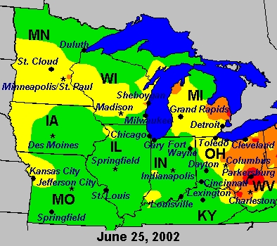
| | - I. Dominion Resources, Inc. (“Dominion”) owns and operates electric generating facilities in eleven states, including the 1250 megawatt coal-fired Kincaid Generation L.L.C. power plant, located in Kincaid, Illinois. Dominion also owns a 50% interest in the 1400-megawatt natural gas-fired Elwood Energy, L.L.C. combustion turbine plant, located in Elwood, Illinois.
- II. Subparts D (CAIR NOx Annual Trading Program) and E (CAIR NOx Ozone Season Trading Program) of the Illinois CAIR proposal deviate significantly from EPA’s model rule and could jeopardize EPA approval of the Illinois CAIR SIP.
- III. The IEPA should justify any “beyond CAIR” NOx reductions with a thorough modeling demonstration.
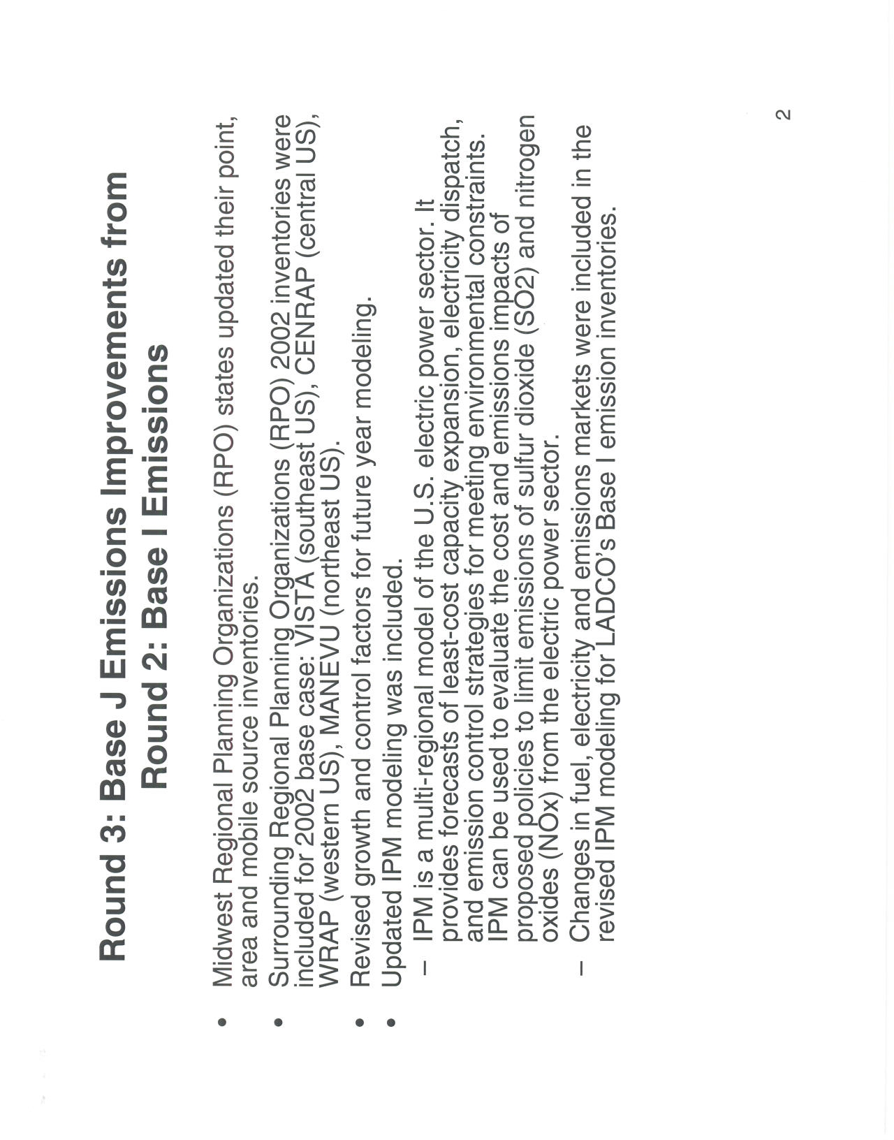
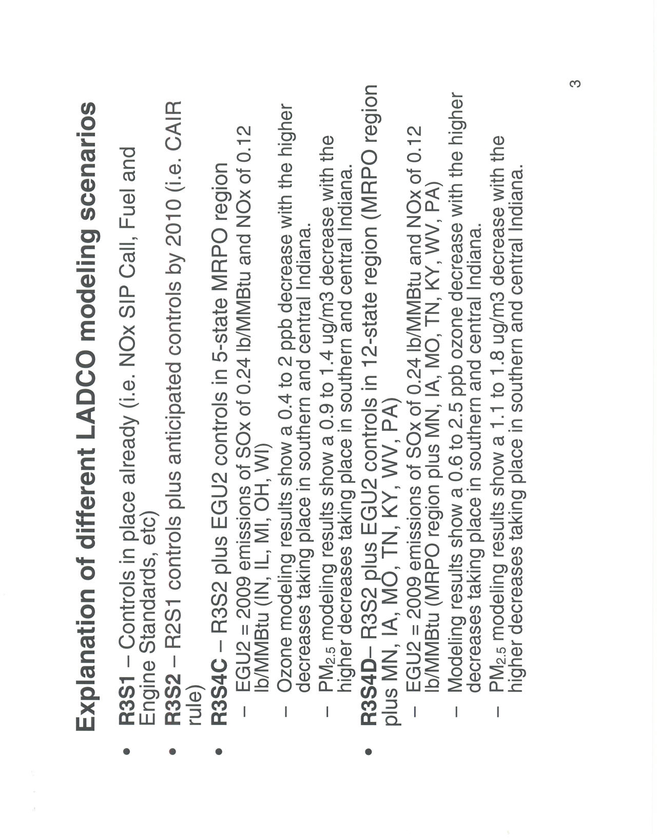
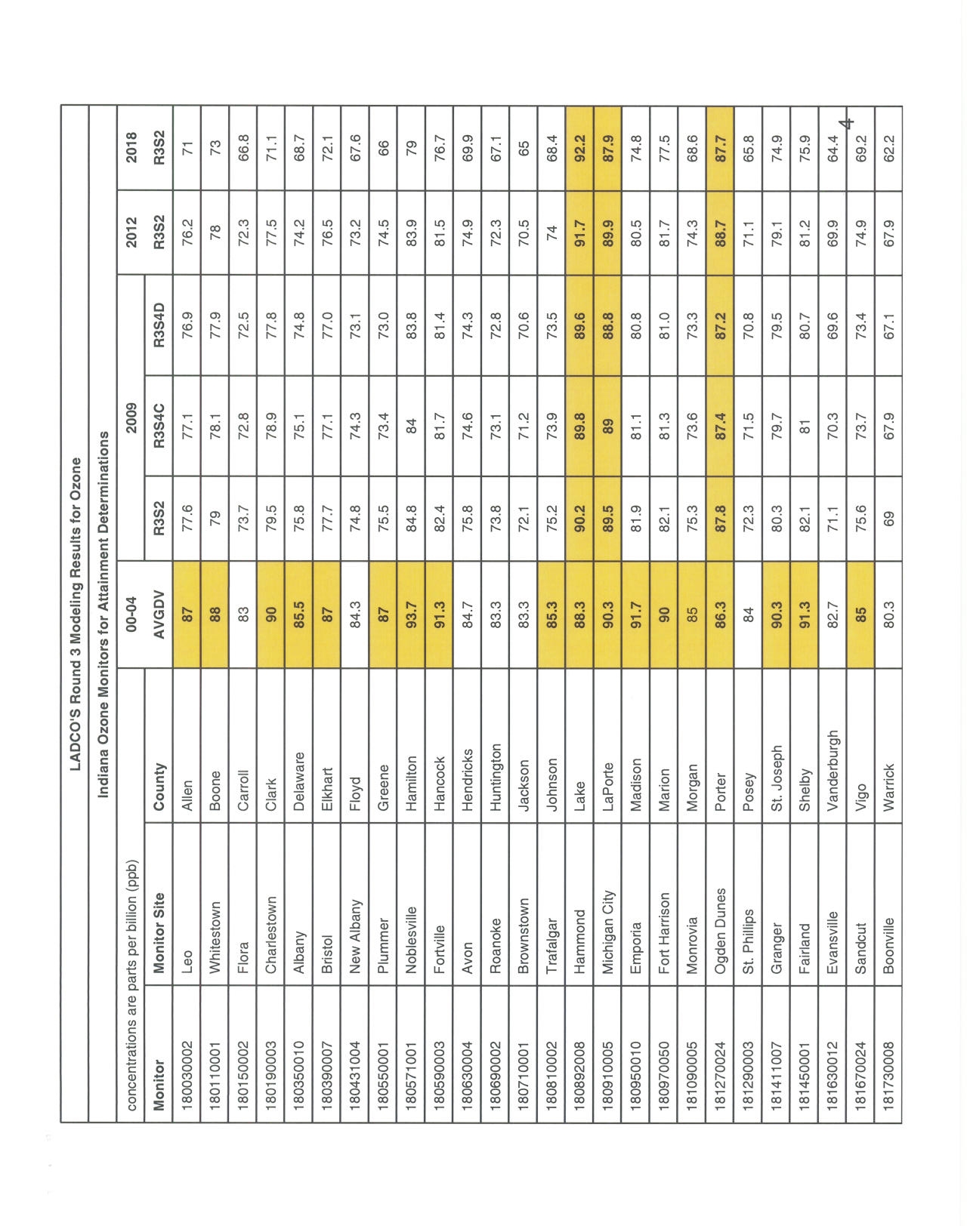
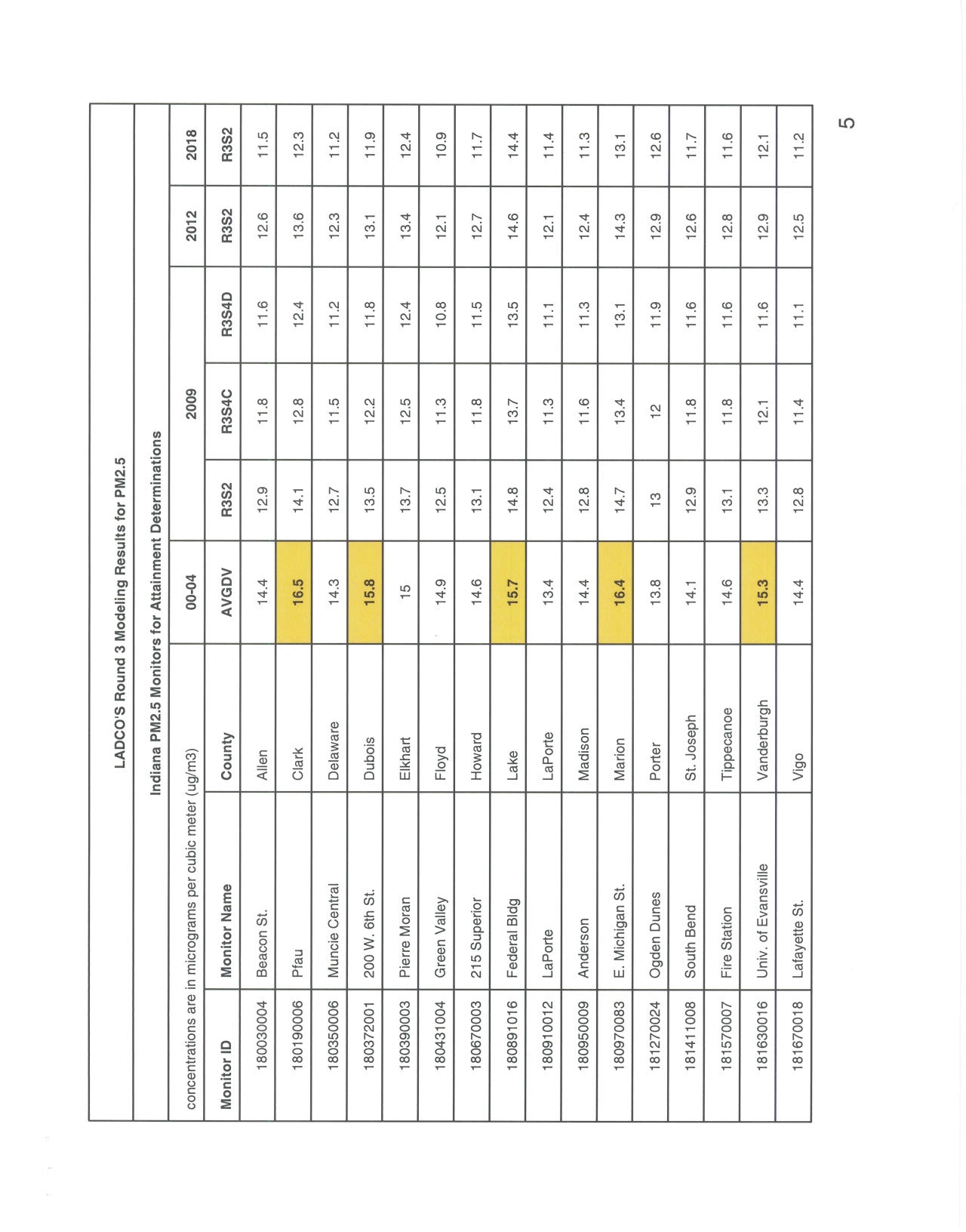
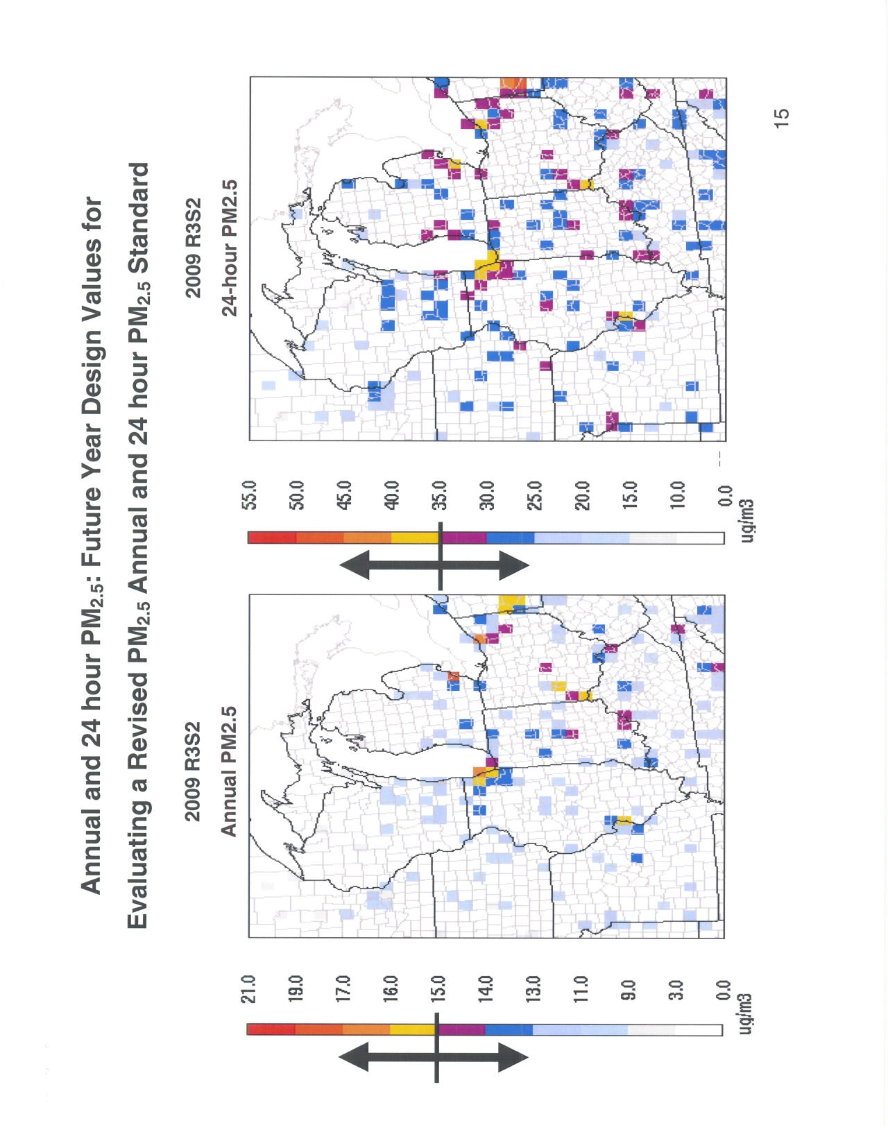
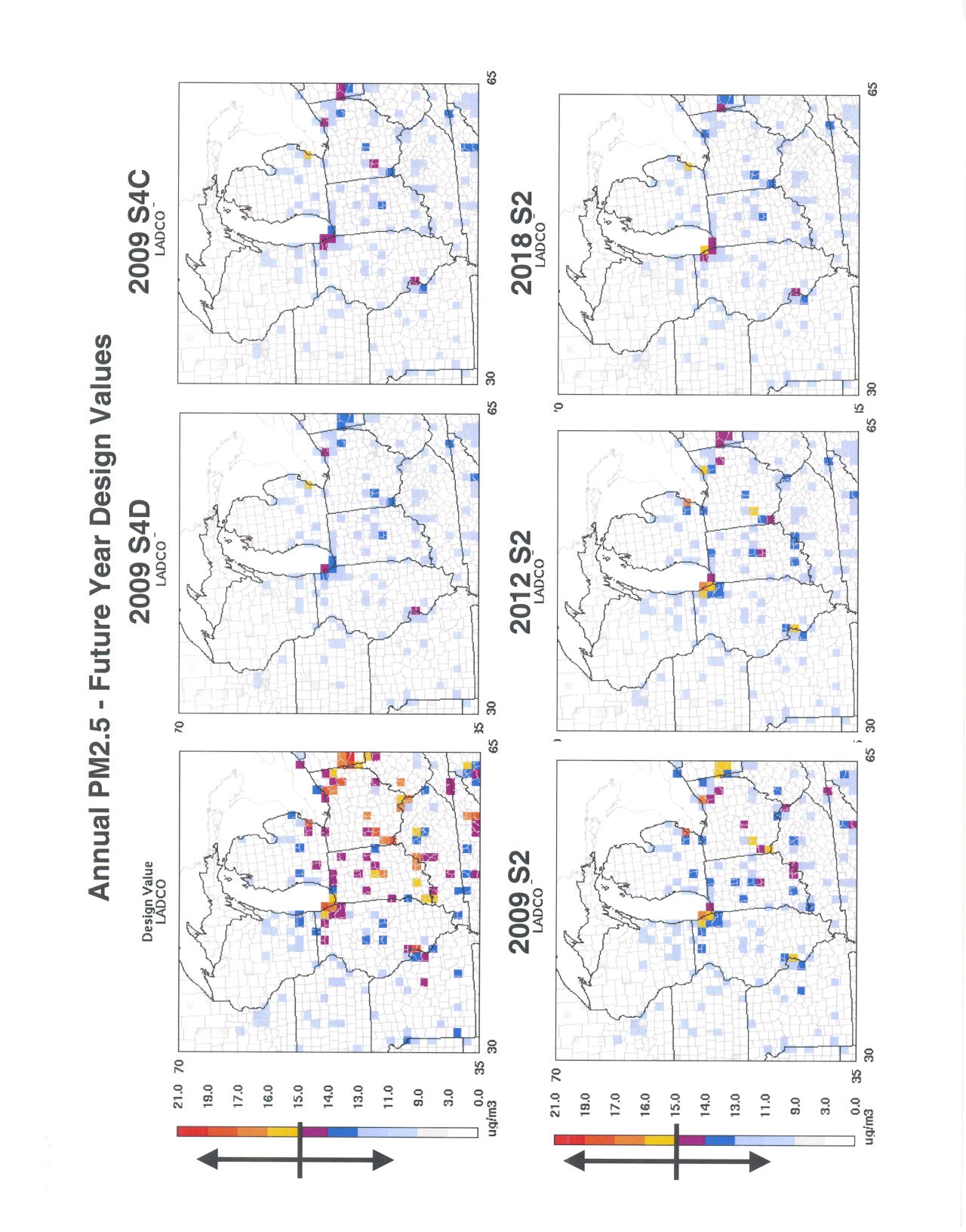
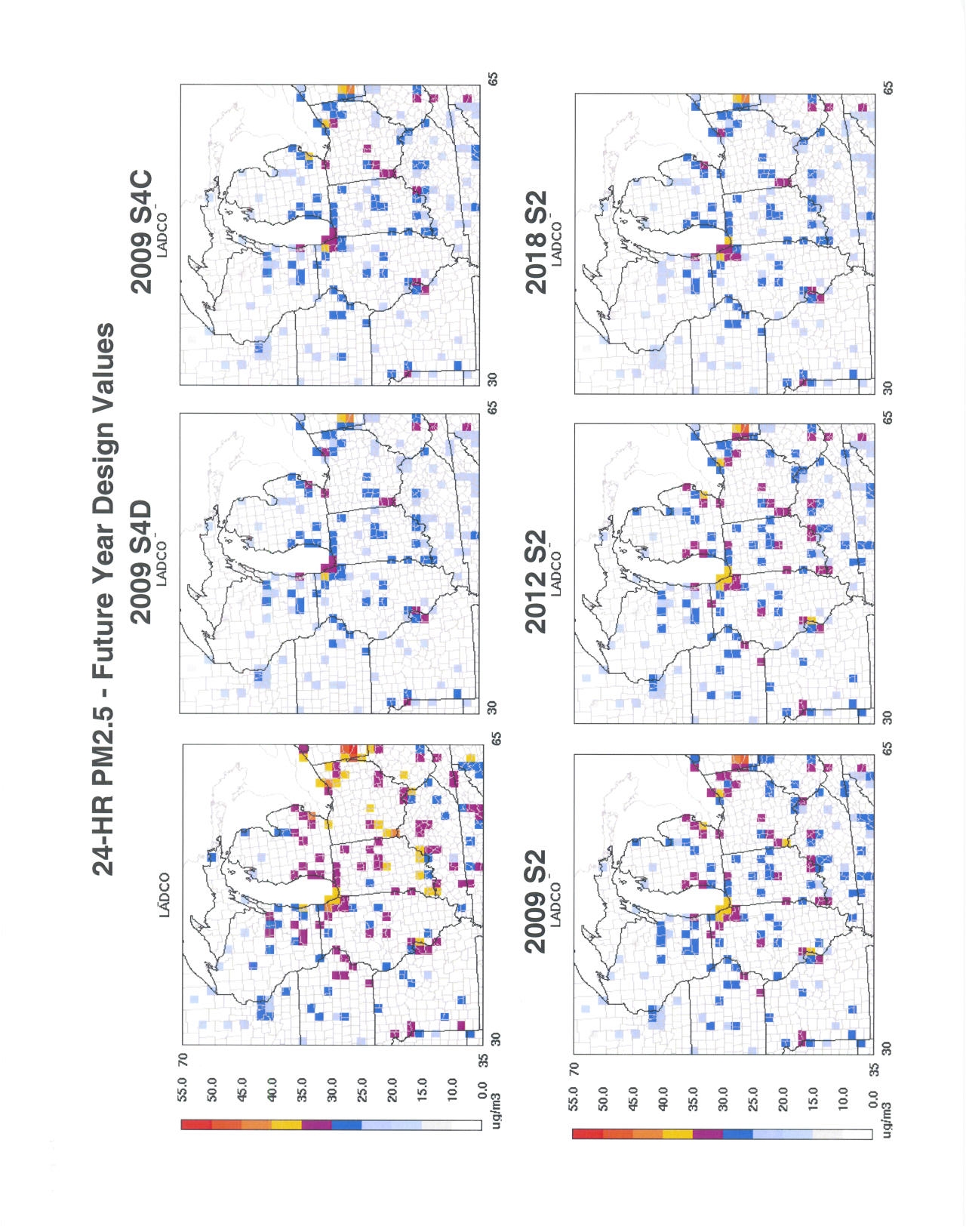
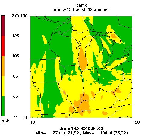
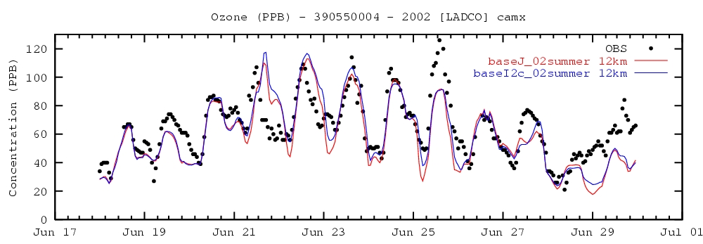
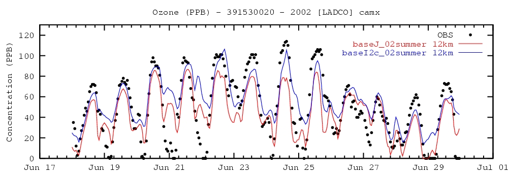
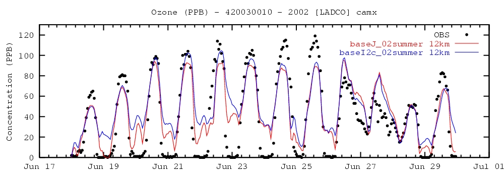
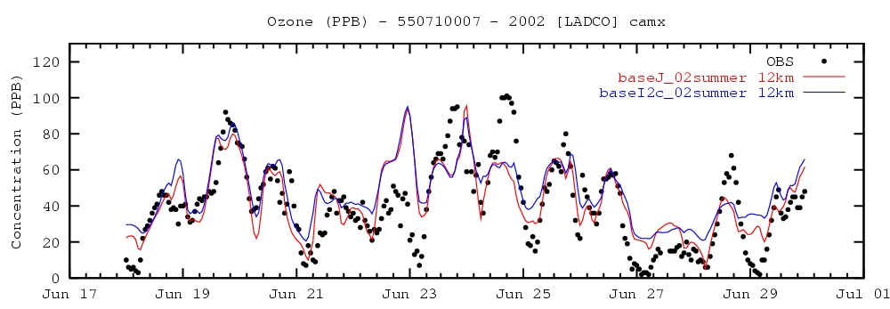
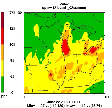
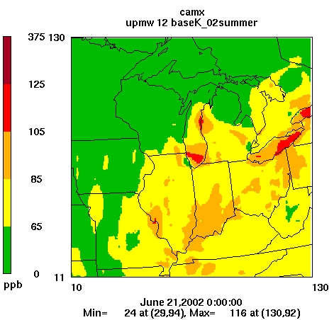
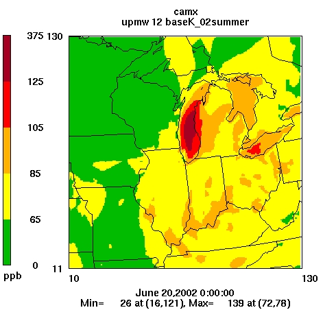
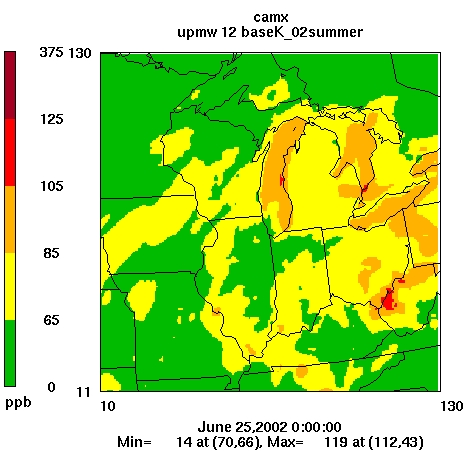
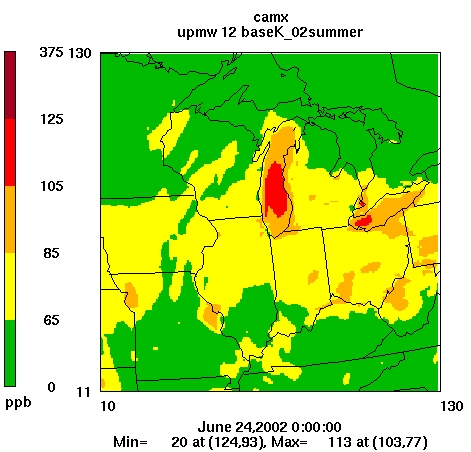
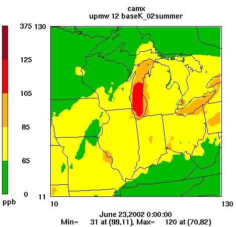
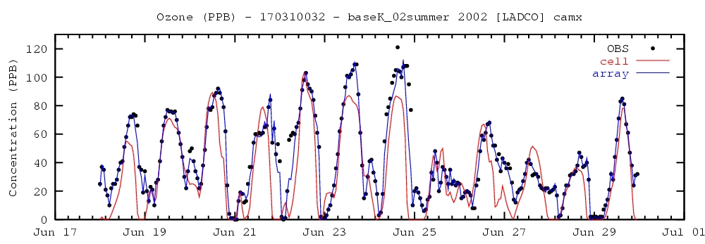
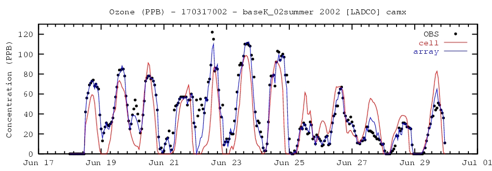
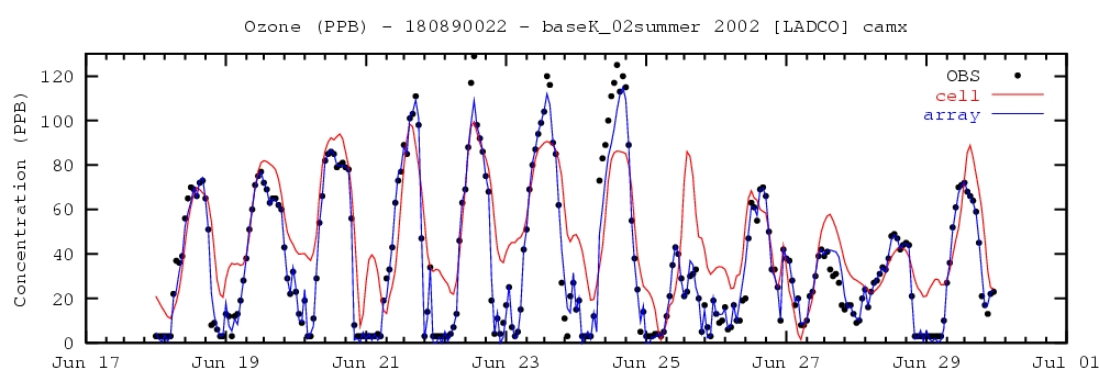
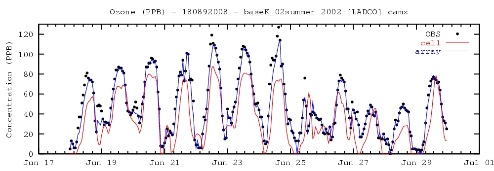
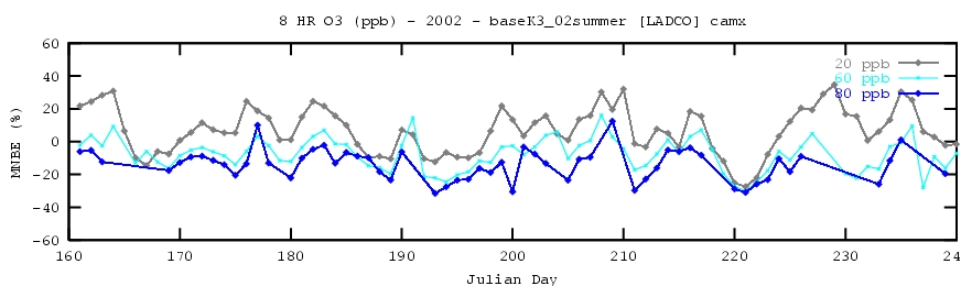
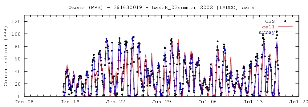
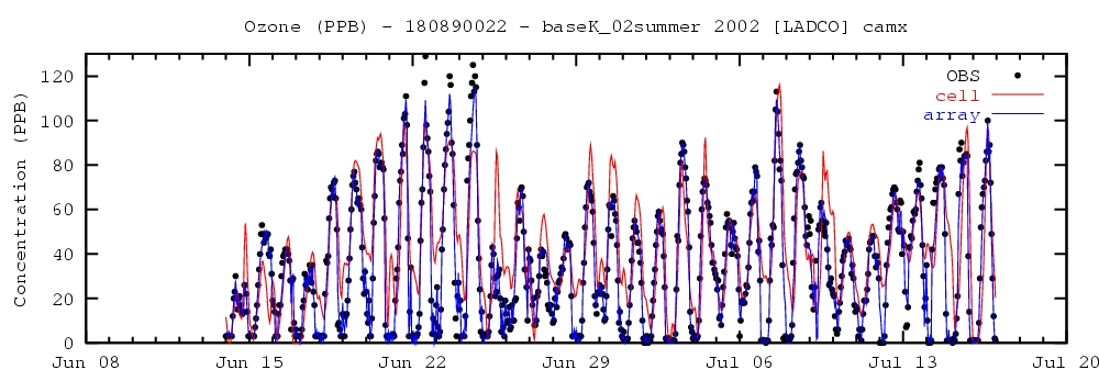
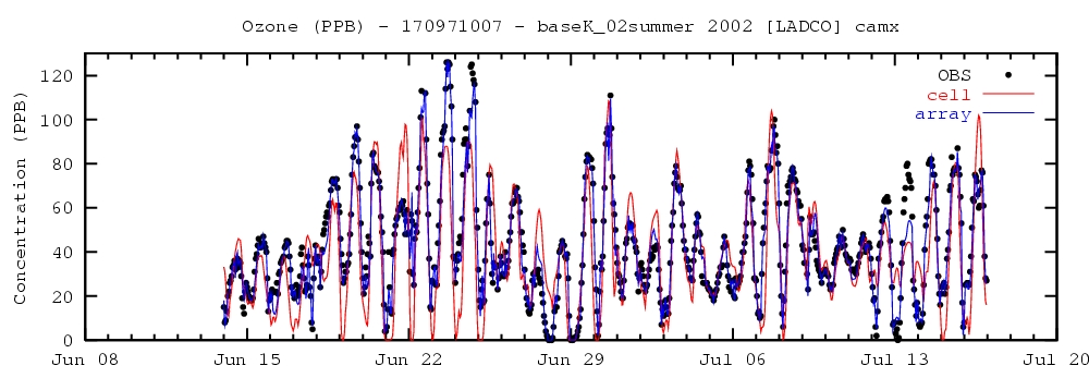
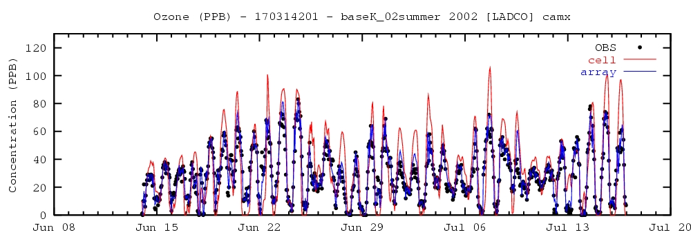
- IV. Recent air quality modeling by Lake Michigan Air Directors Consortium (“LADCO”) suggests additional NOx reductions from the electric generating unit (“EGU”) sector beyond the reductions expected from the federal CAIR program will not solve the residual ozone and PM2.5 non-attainment problem in the Chicago area. A comprehensive attainment plan should be thoroughly researched and fully developed that clearly and conclusively demonstrates the level of emissions reductions needed and the source categories for which the most efficient and effective reductions can be achieved. Only when this plan has been fully developed will IEPA have the justification to proceed with “beyond CAIR” reductions.
- V. The IEPA proposal to adopt “beyond CAIR” NOx reductions through a proposed set-aside program that far surpasses that of any surrounding state places Illinois electricity consumers at a severe economic disadvantage.
- VI. Kincaid supports IEPA’s proposal under Title 35, Part 225, Subpart C to adopt the federal CAIR provisions for SO2.
- VII. Kincaid supports a longer baseline period for determining NOx allocations than proposed by IEPA.
- VIII. Withholding NOx allowances from existing sources, like Kincaid, that have already installed expensive pollution controls to reduce NOx emissions, amounts to a “penalty” for those sources that have opted for this approach. Further, any unclaimed allowances left over in the Energy Efficiency and Conservation/Renewable Energy (“EEC/RE”) set-aside should be returned to the EGUs.
- IX. Kincaid supports USEPA’s position that the CAIR rulemaking does not require states to prepare an attainment SIP to comply with CAIR and the attendant emission reductions are not designed to result in attainment of the NAAQS.
- X. The Board has failed to evaluate the combined impact of CAMR and CAIR.
|
ILLINOIS POLLUTION CONTROL BOARD
In The Matter of:
Proposed New Clean Air Interstate Rule
(CAIR) SO2, NOx Annual and NOx Ozone
Season Trading Programs, 35 Ill. Adm.
Code 225. Subparts A, C, D and E
)
)
)
)
)
No. R06-26
(Rulemaking – Air)
NOTICE OF FILING
TO:
See attached Service List
PLEASE TAKE NOTICE that on January 5, 2007, I caused to be filed electronically with
the Office of the Clerk of the Pollution Control Board, on behalf of KINCAID GENERATION,
L.L.C., the attached KINCAID GENERATION, L.L.C.’S FINAL COMMENTS with
corresponding exhibits, copies of which are hereby served upon you.
By:
/s/ Katherine M. Rahill
Katherine M. Rahill
Bill S. Forcade
Katherine M. Rahill
JENNER & BLOCK LLP
Attorneys for Kincaid Generation, LLC
One IBM Plaza
Chicago, IL 60611
(312) 222-9350
ELECTRONIC FILING, RECEIVED, CLERK'S OFFICE, JANUARY 5, 2007
* * * * * PC #10 * * * * *
CERTIFICATE OF SERVICE
I, Katherine M. Rahill, an attorney, hereby certify that I served copies of the foregoing
documents via first class mail upon the parties on the attached Service List this 5th day of
January, 2007.
By:
/s/ Katherine M. Rahill
Katherine M. Rahill
ELECTRONIC FILING, RECEIVED, CLERK'S OFFICE, JANUARY 5, 2007
* * * * * PC #10 * * * * *
SERVICE LIST:
Dorothy Gunn, Clerk
Illinois Pollution Control Board
James R. Thompson Center
100 W. Randolph St., Suite 11-500
Chicago, IL 60601-3218
John Knittle
Hearing Officer
Illinois Pollution Control Board
James R. Thompson Center
100 W. Randolph, Suite 11-500
Chicago, Illinois 60601
John J. Kim
Rachel L. Doctors
Division of Legal Counsel
Illinois Environmental Protection Agency
1021 North Grand Avenue East
P.O. Box 19276
Springfield, IL 62794-9276
William A. Murray
Special Assistant Corporation Counsel
Office of Public Utilities
800 East Monroe
Springfield, Illinois 62757
Kathleen C. Bassi
Sheldon A. Zabel
Stephen J. Bonebrake
Schiff Hardin LLPP
6600 Sears Tower
233 South Wacker Drive
Chicago, Illinois 60606
Matthew Dunn, Chief
Division of Environmental Enforcement
Office of the Attorney General
188 West Randolph St., 20th Floor
Chicago, IL 60601
Virginia Yang, Deputy Legal Counsel
Illinois Department of Natural Resources
ELECTRONIC FILING, RECEIVED, CLERK'S OFFICE, JANUARY 5, 2007
* * * * * PC #10 * * * * *
One Natural Resources Way
Springfield, IL 62702-1271
Sasha Reyes
Steven Murawski
Baker & McKenzie
One Prudential Plaza, Suite 3500
Chicago, IL 60601
David Rieser
James T. Harrington
Jeremy R. Hojnicki
McGuire Woods LLP
77 West Wacker, Suite 4100
Chicago, Illinois 60601
Faith E. Bugel
Environmental Law and Policy Center
35 East Wacker Drive, Suite 1300
Chicago, Illinois 60601
Keith I. Harley
Chicago Legal Clinic
205 West Monroe Street, 4th Floor
Chicago, Illinois 60606
S. David Farris
Manager, Environmental, Health and Safety
Office of Public Utilities, City of Springfield
201 East Lake Shore Drive
Springfield, Illinois 62757
Bruce Nilles
Sierra Club
122 W. Washington Ave., Suite 830
Madison, WI 53703
Daniel McDevitt
Midwest Generation
440 S. LaSalle Street
Suite 3500
Chicago, IL 60605
ELECTRONIC FILING, RECEIVED, CLERK'S OFFICE, JANUARY 5, 2007
* * * * * PC #10 * * * * *
BEFORE THE ILLINOIS POLLUTION CONTROL BOARD
In The Matter of:
Proposed New Clean Air Interstate Rule
(CAIR) SO2, NOx Annual and NOx Ozone Season
Trading Programs, 35 Ill. Adm. Code 225.
Subparts A, C, D and E.
)
)
)
)
)
No. R06-26
(Rulemaking -Air)
FINAL COMMENTS OF KINCAID GENERATION, L.LC.
NOW COMES Participant KINCAID GENERATION, L.L.C. (“Kincaid”), by and
through its attorneys, JENNER & BLOCK LLP, and respectfully submits its final comments to
this rulemaking. Kincaid appreciates this opportunity to comment again on these important new
rules. Kincaid has been an active participant throughout this long rulemaking process –
attending all the “outreach” meetings convened by the Illinois Environmental Protection Agency
(“IEPA”) in Springfield in January and February, participating in the Board hearings both in
Springfield and Chicago, providing comment on the proposal on two separate occasions, and
providing testimony at the Chicago hearing.
I.
Dominion Resources, Inc. (“Dominion”) owns and operates electric generating
facilities in eleven states, including the 1250 megawatt coal-fired Kincaid
Generation L.L.C. power plant, located in Kincaid, Illinois. Dominion also owns a
50% interest in the 1400-megawatt natural gas-fired Elwood Energy, L.L.C.
combustion turbine plant, located in Elwood, Illinois.
Over the past eight years, Dominion’s Kincaid station has been installing pollution controls,
switching fuels and making other changes to ensure compliance with the increasingly more
stringent air quality emissions limitations. To reduce sulfur dioxide emissions in order to
comply with Phase II of the federal Acid Rain program, Kincaid switched in 1999 to the much
ELECTRONIC FILING, RECEIVED, CLERK'S OFFICE, JANUARY 5, 2007
* * * * * PC #10 * * * * *
2
lower sulfur Powder River Basin (“PRB”) coal. In 2001, Kincaid began construction of two
selective catalytic reduction (“SCR”) systems to control nitrogen oxides (“NO
x
”) emissions as
part of the Illinois NO
x
requirements under the new IEPA Subpart W regulations. These massive
control devices began operation in 2003 and have been very effective, reducing ozone season
NO
x
emissions by more than 85% from previous levels.
Kincaid supports the adoption of state regulations that embrace the federal Clean Air Interstate
Rule (“CAIR”). Kincaid appreciates the IEPA’s efforts to address the individual electric
companies’ particular problems associated with implementation of these important new
regulations and also appreciates this opportunity to comment on the proposed regulations.
II.
Subparts D (CAIR NO
x
Annual Trading Program) and E (CAIR NO
x
Ozone Season
Trading Program) of the Illinois CAIR proposal deviate significantly from EPA’s
model rule and could jeopardize EPA approval of the Illinois CAIR SIP.
Kincaid does not support the IEPA proposal under Subparts D and E. Specifically, we do not
support the 25% set-aside of NO
x
allowances under proposed Sections 225.455 and 225.555, the
so-called “Clean Air Set-Aside” (“CASA”). First, the agency has provided no justification that
the level of the proposed set-aside is necessary from an air quality perspective. Second, these
provisions will significantly increase compliance costs for Illinois sources and competitively
disadvantage the state relative to surrounding states. Furthermore, this approach also could
jeopardize USEPA approval of the Illinois CAIR SIP, and perhaps the ability of Illinois sources
to participate in the federal trading program. It may also deny Illinois the economic advantages
of the USEPA trading program that many other surrounding states will realize through their
adoption of the USEPA rule.
ELECTRONIC FILING, RECEIVED, CLERK'S OFFICE, JANUARY 5, 2007
* * * * * PC #10 * * * * *
3
In addition, we do not support the proposed withholding of allowances from the compliance
supplement pool (“CSP”) under Section 225.480 of the CAIR NO
x
Annual Trading Program
proposal. These additional NOx allowances have been provided in the federal rule to encourage
early reductions during 2007 and 2008. Illinois included early reduction provisions in its rules
implementing the NO
x
SIP Call. These early reduction incentives not only provide companies
added compliance flexibility that eases the burden once the requirements take effect, but benefit
the environment as well by providing real emission reductions sooner. Given this past success, it
seems counterintuitive for the agency to consider eliminating such an incentive by withholding
allowances from the CSP.
III.
The IEPA should justify any “beyond CAIR” NO
x
reductions with a thorough
modeling demonstration.
Should there remain local areas in Illinois that fail to meet the air quality standards following
implementation of the CAIR regional reductions, the IEPA should thoroughly evaluate the
amount of additional air quality improvement needed and the amount of emission reductions
needed in the more localized nonattainment area in order to achieve the needed air quality
improvements in the most cost-effective manner. Requiring all Illinois sources subject to CAIR
to implement “beyond CAIR” reductions across-the-board for the purpose of resolving local
problems is not reasonable or environmentally justified. Kincaid urges IEPA to conduct a
thorough modeling demonstration to determine the level of reductions that may be necessary to
resolve any residual non-attainment problems following implementation of the CAIR reductions.
The 25% NO
x
“set-aside” is unreasonably burdensome to Illinois generators and their customers
and has not been demonstrated to be necessary to achieve attainment with the ambient air quality
ELECTRONIC FILING, RECEIVED, CLERK'S OFFICE, JANUARY 5, 2007
* * * * * PC #10 * * * * *
4
standards. As USEPA has stated, the program is designed “to balance the burden for achieving
attainment between regional-scale and local-scale control programs.”
1
Therefore, for the purposes of implementation of CAIR, Kincaid does not believe it is necessary
for IEPA to propose the “beyond CAIR” NO
x
reductions and urges the Board to reject the IEPA
proposal and, instead, approve full adoption of USEPA’s federal “model rule” on the same
schedule established by USEPA.
IV.
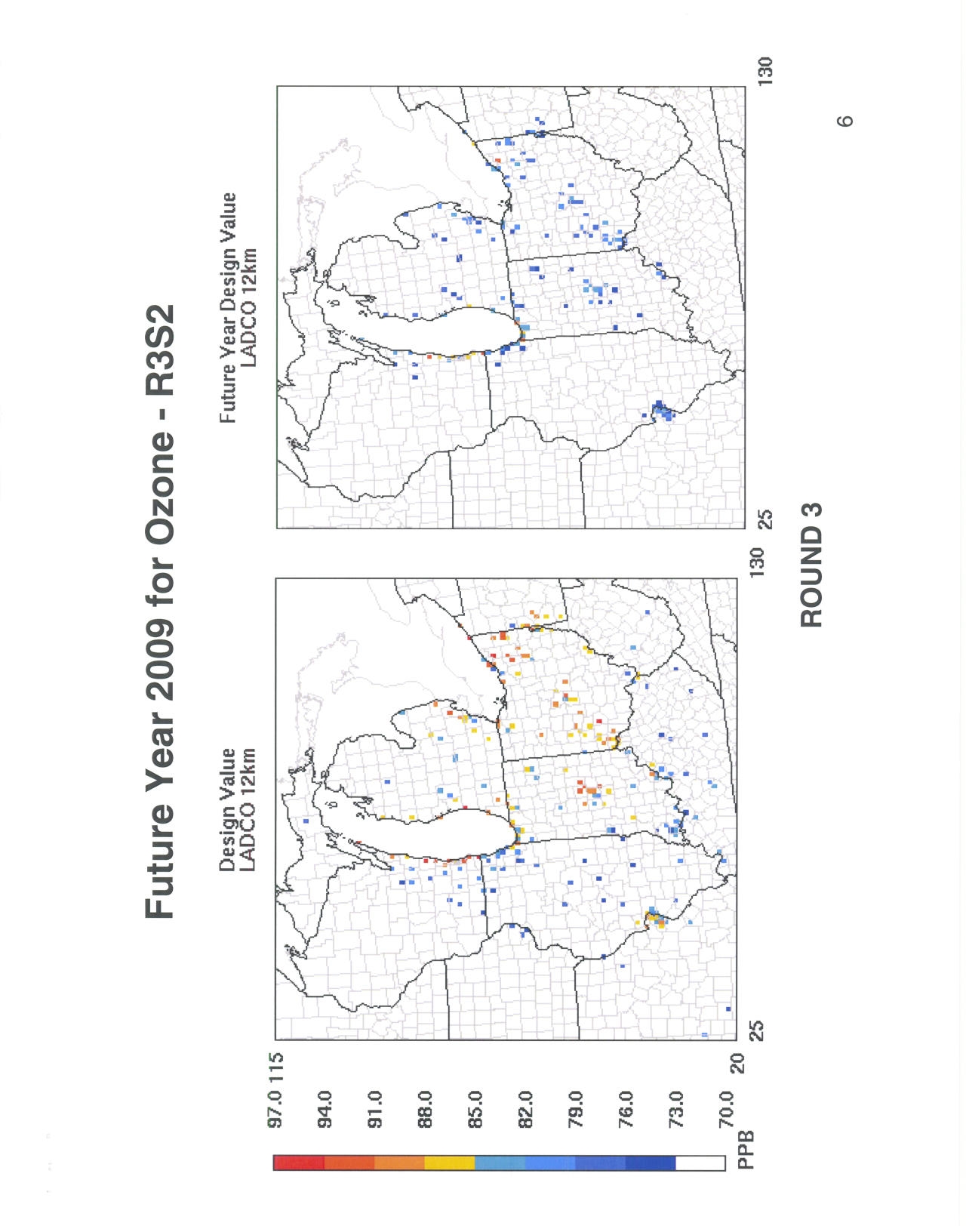
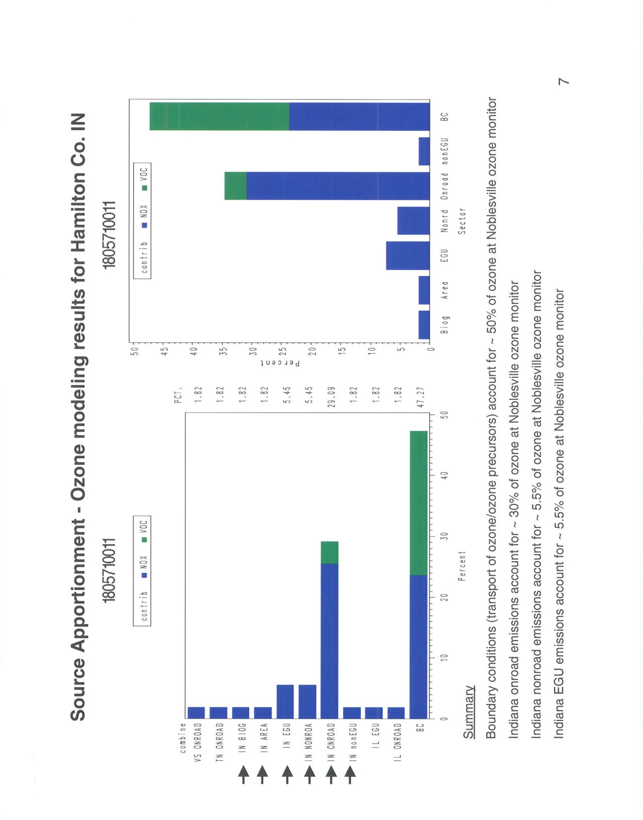
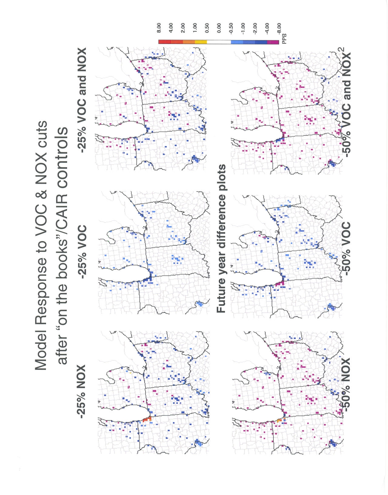
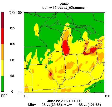
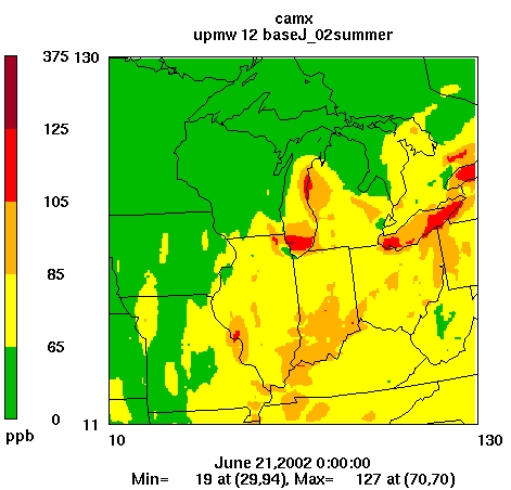
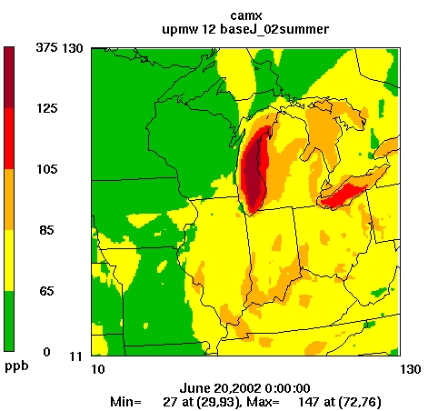
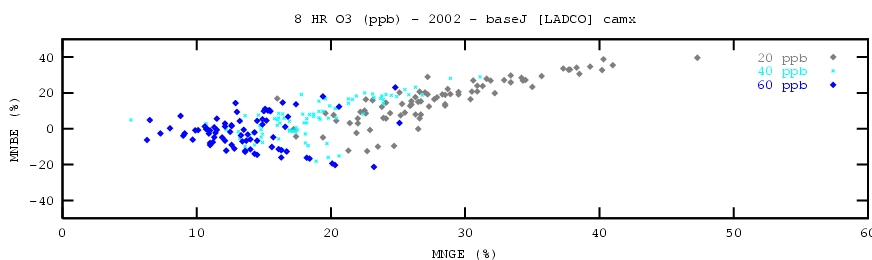
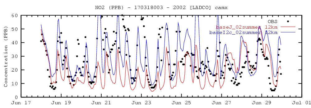
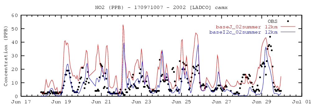
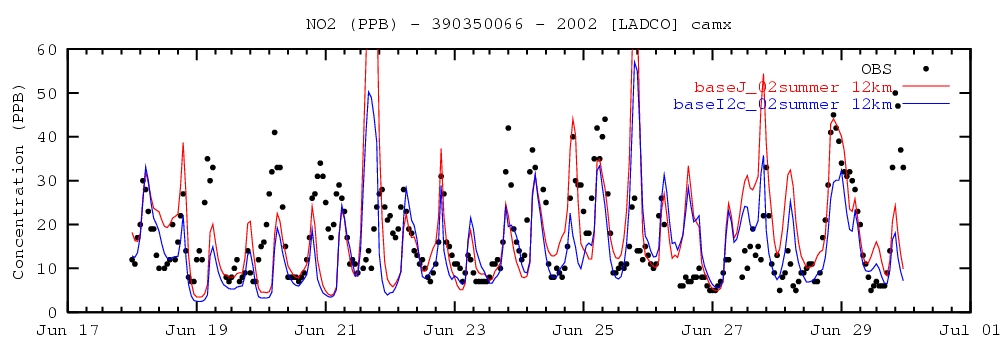
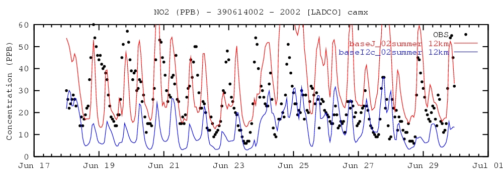
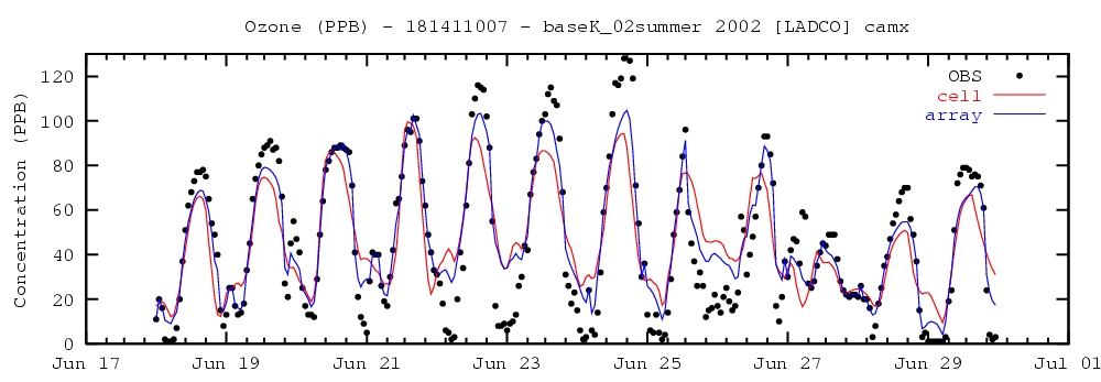
Recent air quality modeling by Lake Michigan Air Directors Consortium
(“LADCO”) suggests additional NO
x
reductions from the electric generating unit
(“EGU”) sector beyond the reductions expected from the federal CAIR program
will not solve the residual ozone and PM
2.5
non-attainment problem in the Chicago
area. A comprehensive attainment plan should be thoroughly researched and fully
developed that clearly and conclusively demonstrates the level of emissions
reductions needed and the source categories for which the most efficient and
effective reductions can be achieved. Only when this plan has been fully developed
will IEPA have the justification to proceed with “beyond CAIR” reductions.
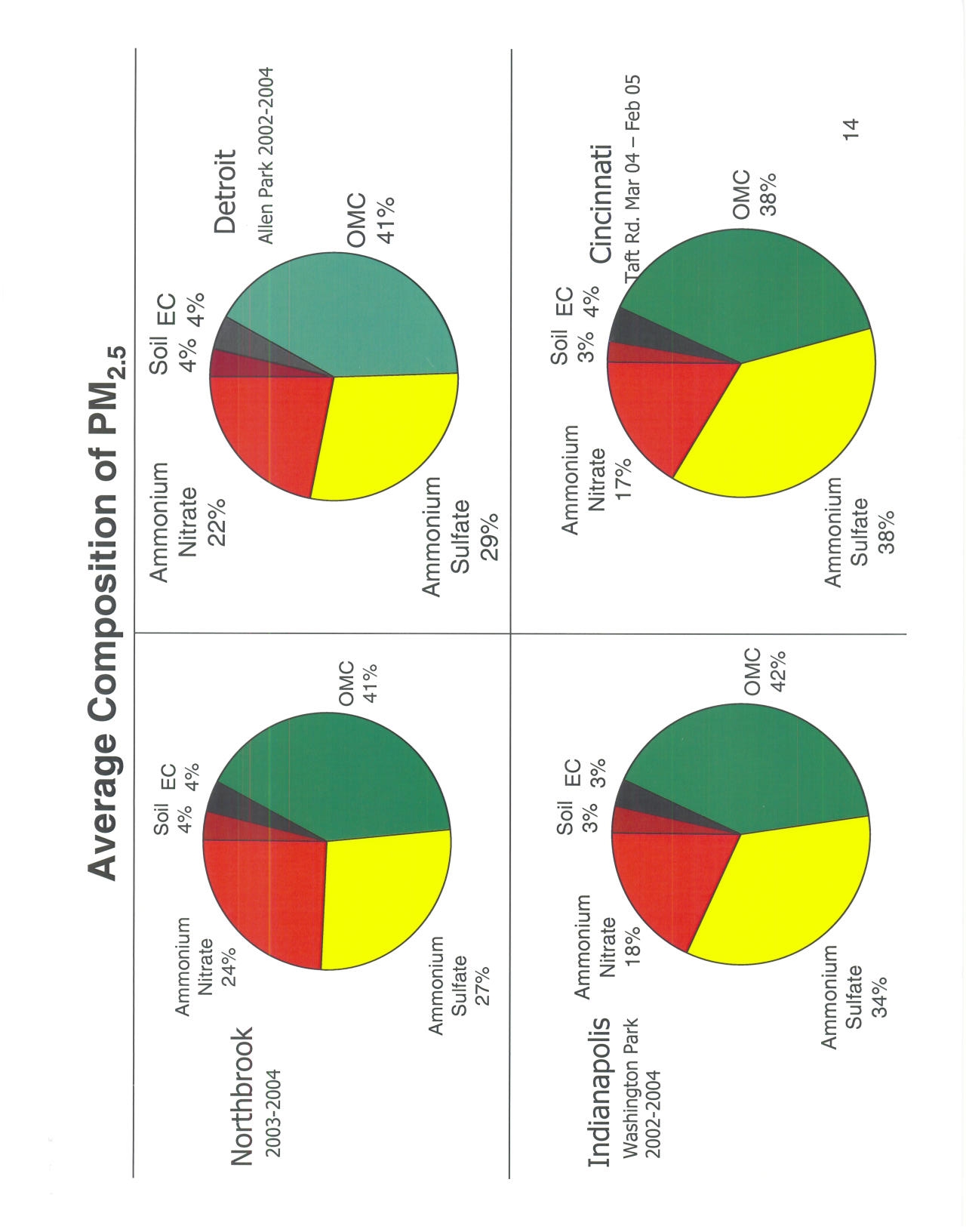
Further EGU reductions of SO
2
and NO
x
are not likely to impact PM
2.5
concentrations
sufficiently to achieve attainment in any residual PM
2.5
nonattainment areas in Illinois or in other
states. Accordingly, mandated beyond-CAIR EGU reductions of SO
2
and NO
x
may not be
necessary, cost effective or even have any beneficial effect on reducing the particle concentration
of monitored PM
2.5
. The PM
2.5
particle composition may well be driven by mobile sources in
winter. Another source mix may drive the PM
2.5
composition in summer. Until additional
speciated monitoring data is available, it is premature to require “beyond CAIR” SO
2
or NO
x
reductions from EGUs because the absolute value of PM
2.5
concentrations measured in the field
may not be driven by SO
2
or NO
x
reductions.
1
70 Fed. Reg. 25166 (May 12, 2005)
ELECTRONIC FILING, RECEIVED, CLERK'S OFFICE, JANUARY 5, 2007
* * * * * PC #10 * * * * *
5
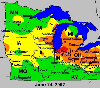
Kincaid recognizes that several areas, including the Chicago MSA, may not achieve one or both
of these standards following the implementation of Phase 2 of CAIR in 2015. Although the
Chicago MSA, while closer to attainment, still may not reach attainment for ozone or PM
2.5
, it
appears that further regional reductions in the utility sector do not make a significant difference
in the attainment status of the Chicago MSA. Indeed, based on one analysis presented at the
October 18, 2005 Indiana Department of Environmental Management Utility Rules Workgroup
meeting, further reductions in the utility sector actually cause ozone levels to increase in the
Chicago MSA. Kincaid therefore supports the approach to implement CAIR essentially as
established by USEPA, and then work with sources in local nonattainment areas to determine the
appropriate mix of reductions needed to resolve the remaining local nonattainment area issues.
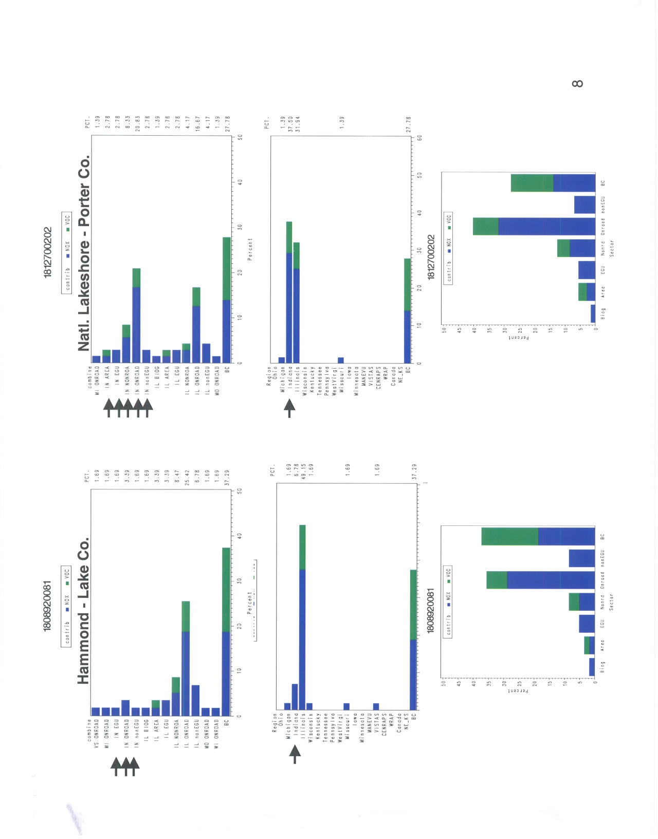
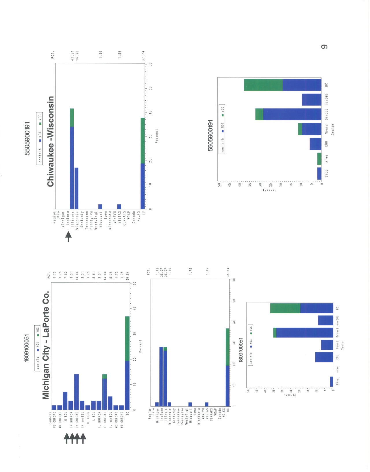
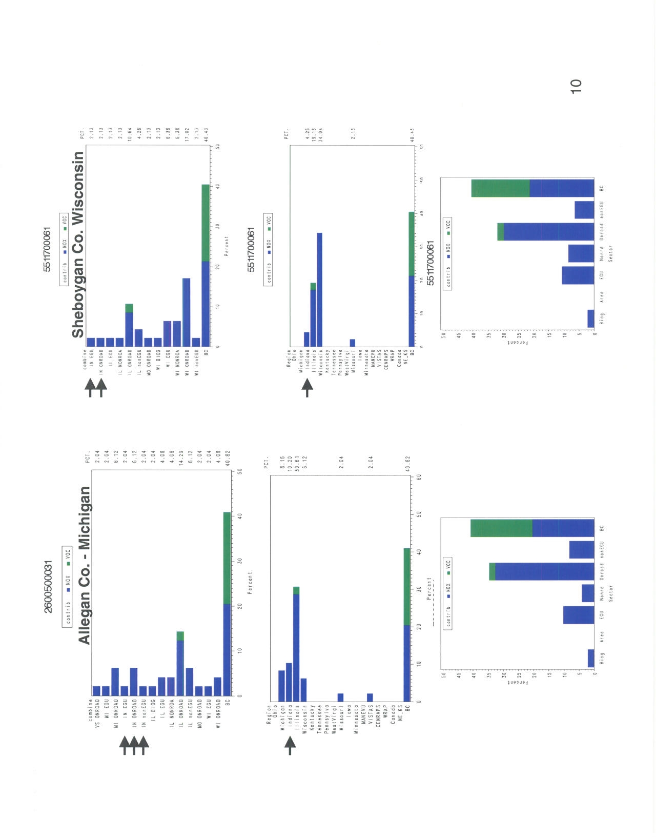
Source apportionment data provided by LADCO bears this reasoning out. Data presented at the
October 18, 2005 Indiana Utility Rules Workgroup meeting clearly indicates that Illinois EGUs
make up only a small part of the ozone non-attainment problem in Chicago MSA. The data
indicate that 38% of the ozone comes from NO
x
and VOC emissions from “Boundary
Conditions” or sources outside the five-state Midwest region. More important, 26% of the ozone
problem appears to come from “Illinois On-road” or mobile sources. Illinois EGU NO
x
emissions make up only about 4% of the ozone contribution, behind “Illinois Non-road,”
“Illinois Non-EGU,” and “Indiana On-road” sources.
2
2
Mark Derf, “Photochemical Modeling Update: Round 3 – 8 Hour Ozone and PM
2.5
,” Presentation for the Utility
Rules Workgroup, Indiana Department of Environmental Management, October 18, 2005, attached as Exhibit A.
ELECTRONIC FILING, RECEIVED, CLERK'S OFFICE, JANUARY 5, 2007
* * * * * PC #10 * * * * *
6
V.
The IEPA proposal to adopt “beyond CAIR” NO
x
reductions through a proposed
set-aside program that far surpasses that of any surrounding state places Illinois
electricity consumers at a severe economic disadvantage.
The proposal to allocate 25% of Illinois’ annual NO
x
budget as “set-asides” for the CASA
allowances will severely restrict NO
x
allocations for affected units. There appears to be little
chance that these allowances will ever be returned to the EGUs since the proposal calls for any
NO
x
allowances that remain unclaimed from the four CASA allowance pools (Energy Efficiency
and Conservation/Renewable Energy; Air Pollution Control Equipment Upgrades; Clean Coal
Technology; and Early Adopters) to be used to replenish each of the four CASA pools. Once the
allowances in each of these pools are replenished to a level twice the amount originally
designated for that pool, proposed section 225.475 (and section 225.575 of the Ozone Season
rule) indicates “the Agency may elect to retire the CAIR NOx allowances that have not been
distributed…” Thus, the 25% set-aside essentially becomes a 25% reduction beyond the NO
x
limits in the federal CAIR rule. The equivalent NO
x
limit is very close to the NO
x
limit
suggested by LADCO as modeling scenario “EGU1.”
Recent studies have evaluated the economic impacts that the imposition of broad-based “beyond-
CAIR” model rule reductions on EGU sources would have on the State of Illinois. An August
26, 2005 report prepared by BBC Research & Consulting (“BBC”) of Denver, Colorado, for the
Midwest Ozone Group and the Center for Energy and Economic Development indicates that
imposition of “beyond-CAIR” control strategies, such as the ones described in the white paper
prepared by LADCO on additional control scenarios for EGUs, could have a significant negative
impact on the economies of several Midwestern states. The paper examined two scenarios
referred to as “EGU1” and “EGU2.” The BBC results indicate that imposition of these “beyond
ELECTRONIC FILING, RECEIVED, CLERK'S OFFICE, JANUARY 5, 2007
* * * * * PC #10 * * * * *
7
CAIR” requirements on EGUs will result in the mandatory requirement of installation of controls
on very small units.
3
BBC estimated the electric rate impacts of the proposed LADCO controls and the corresponding
impact of higher electric rates on the case study industries and on household spending in the five
states within the LADCO region. Rate impacts were estimated by comparing the projected
annual electric utility revenue requirements, including costs of compliance with the LADCO
controls, with projected annual electric utility revenue requirements after compliance with
CAIR. BBC examined several scenarios of LADCO controls, including with and without
replacement power to compensate for early generating unit retirements under EGU1 and EGU2.
BBC quantified overall effects on regional output and employment arising from the direct
impacts on the case study industries and from the impacts of higher electric rates on household
disposable income. Impacts were quantified using partial equilibrium analyses of each case
study industry along with the IMPLAN economic input-output model. The focus of the study
was on the direct and secondary (or “multiplier”) effects on ten case study industries and on the
portions of the economy supported by household spending. The findings of BBC are
conservative, i.e., are underestimated, because impacts of higher electric rates on other industries
and the commercial sector (which together account for about one-third of all electricity sales)
were not included. Health- and visibility-related economic benefits of emissions reductions and
the potential short-term economic effects on the construction industry from building and
installing pollution control equipment were also outside the scope of the BBC study. It should
3
“Midwest Electric Rate Impact Study,” BBC Research and Consulting, Denver, Colorado, August 26, 2005,
attached as Exhibit B.
ELECTRONIC FILING, RECEIVED, CLERK'S OFFICE, JANUARY 5, 2007
* * * * * PC #10 * * * * *
8
be noted that the BBC study has evaluated economic impacts of the LADCO EGU1 and EGU2
scenarios that includes tighter SO
2
emissions limits, which make up the majority of these costs.
Key findings of the BBC report are as follows:
1. From a regional standpoint, electric rates in the year 2013 would be about 11 percent
higher under EGU1 and 16 percent higher under EGU2 than under the CAIR Rule.
Electric rates would increase in Illinois by about 9 percent under EGU1 and about 15
percent under EGU2.
2. Demand for coal mined in Illinois, Indiana and Ohio is expected to decline by 48 percent
under EGU1 and 54 percent under EGU2.
3. Annual economic output in the five-state region is projected to be reduced by between
$6.9 billion and $10.4 billion under EGU1 and between $9.0 billion and $14.1 billion
under EGU2. The economic output of Illinois could fall by up to $2.0 billion in the year
2013.
4. Employment in the five-state region is projected to be reduced by approximately 51,000
to 69,000 jobs under EGU1 and 69,000 to 94,000 under EGU2. In Illinois, the estimated
job loss ranges from 9,300 to 12,100 under EGU1 and between 13,400 and 17,600 under
EGU2.
Kincaid has attempted to separate the estimated costs presented in the BBC report for
compliance with only the NO
x
provisions of an EGU1 scenario. While Kincaid cannot at this
time provide a breakdown of the state-specific costs associated with the EGU1 NO
x
reductions
ELECTRONIC FILING, RECEIVED, CLERK'S OFFICE, JANUARY 5, 2007
* * * * * PC #10 * * * * *
9
expected for Illinois, Kincaid can provide an estimated cost for the five-state Midwest region
(Illinois, Indiana, Ohio, Michigan and Wisconsin). Kincaid consulted the analysts that provided
the cost data that BBC used as input to their report and their projection for the NO
x
portion of the
EGU1 scenario was estimated at $865 million per year.
4
Illinois’ share of these costs will be
borne by the citizens and industries of Illinois – costs that states adopting the federal CAIR
program will not have to bear.
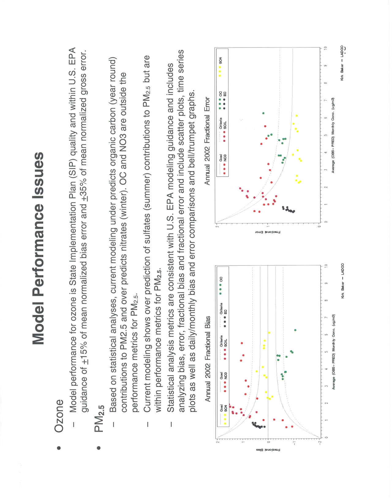
VI.
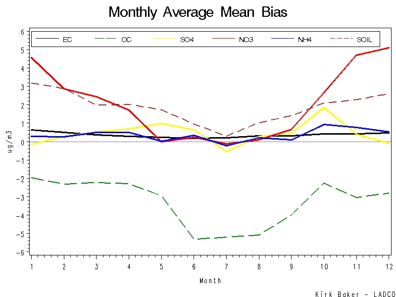
Kincaid supports IEPA’s proposal under Title 35, Part 225, Subpart C to adopt the
federal CAIR provisions for SO
2
.
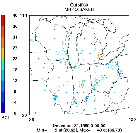
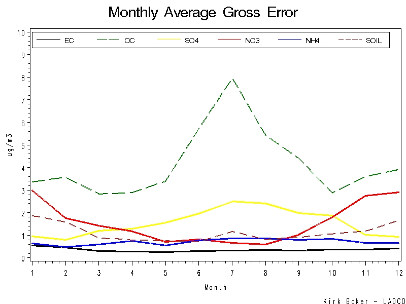
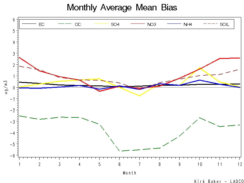
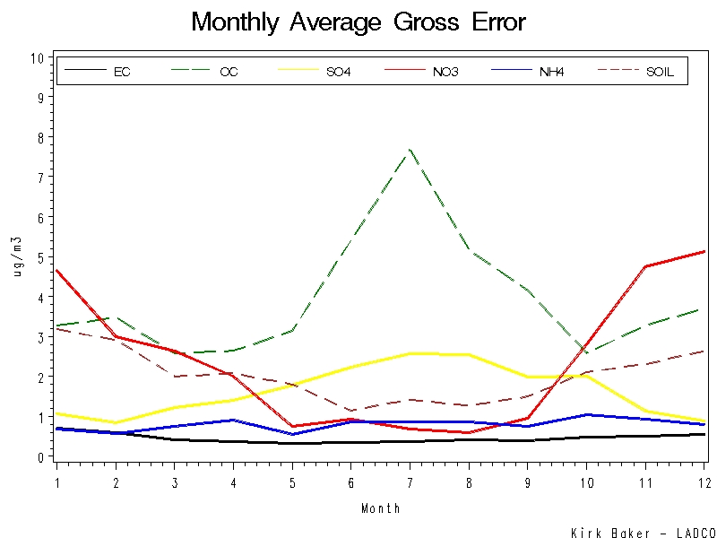
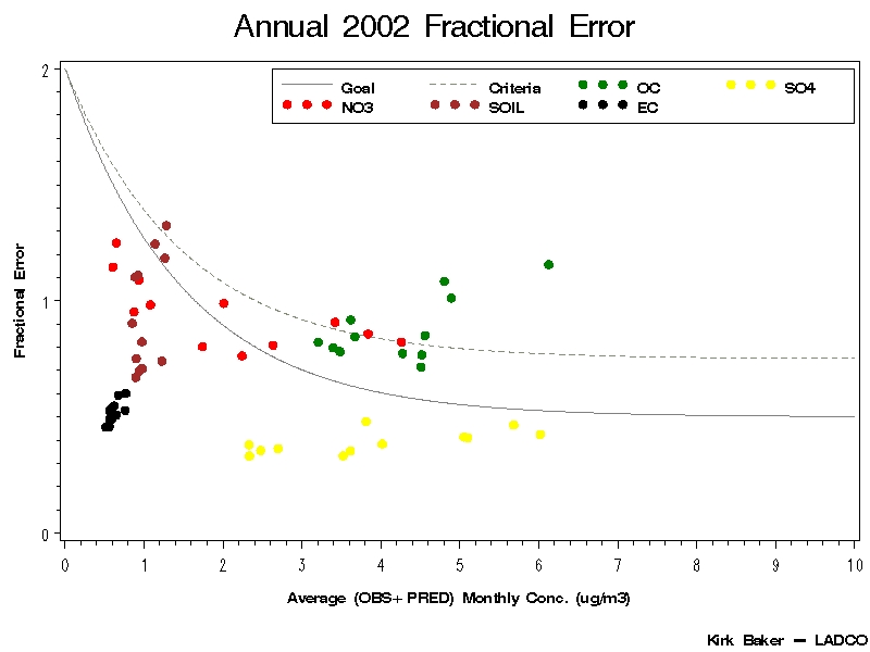
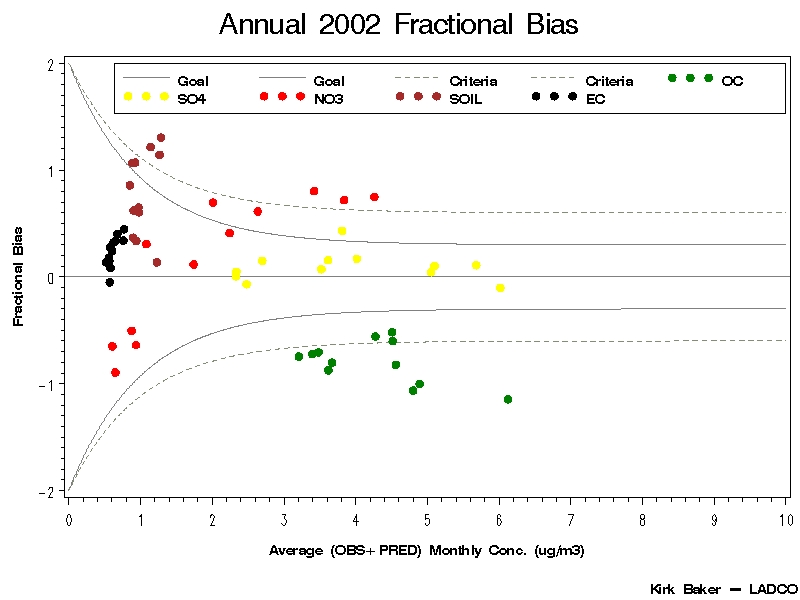
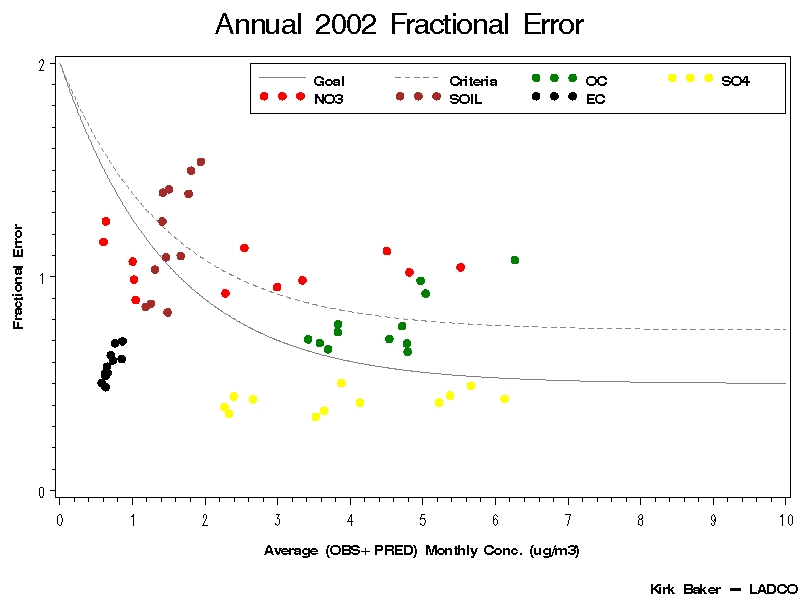
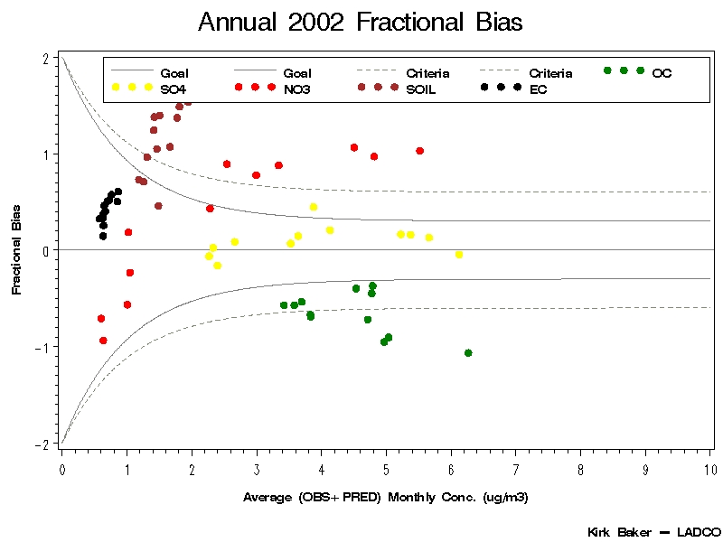
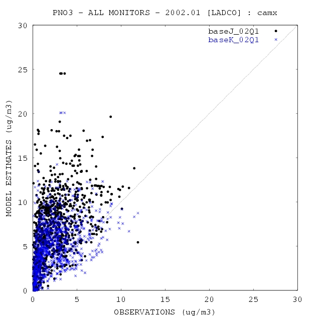
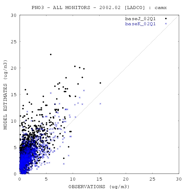
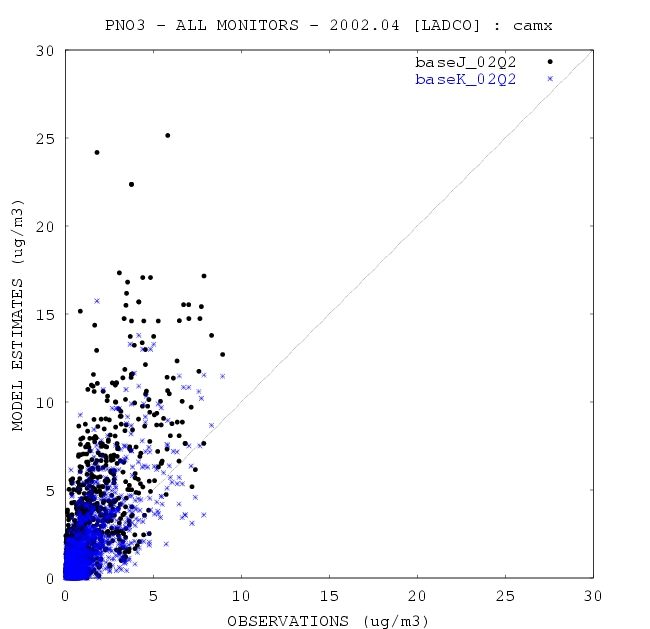
Kincaid supports the IEPA proposal to adopt the federal CAIR SO
2
Trading Program as part of
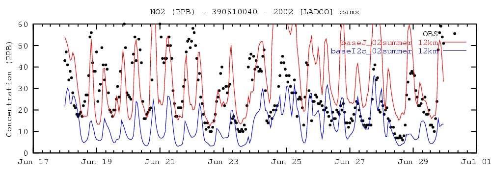
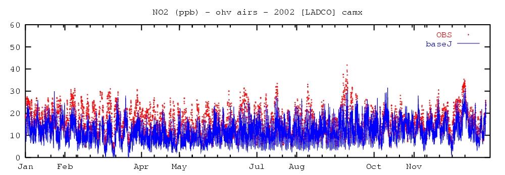
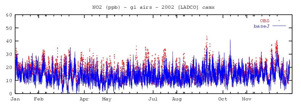
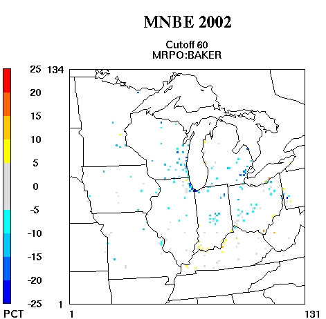
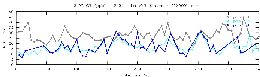
the Illinois CAIR rule. Modeling conducted by LADCO in the fall of 2005 suggests the current
PM
2.5
models are not yet sufficiently accurate to base regulatory decisions on. LADCO indicates
the model “over predicts” the contribution of sulfates to PM
2.5
concentrations and “under
predicts” the contribution from organic carbon.
5
The organic carbon contribution continues to
be a problem with the most recent LADCO PM
2.5
model performance, described by LADCO as
“very poor.”
6
4
James Marchetti, Michael Hein and J. Edward Cichanowicz, “Evaluation of the Midwest RPO Interim Measures
and EGU1 and EGU2” – presented at the June 28, 2005 Midwest Regional Planning Organization Regional
Workshop, attached as Exhibit C.
5
Kirk Baker, LADCO Round 3 (Base J) Model Performance, September 2005, attached as Exhibit D.
6
Kirk Baker, LADCO Round 4 (Base K) Model Performance, April 2006, attached as Exhibit E.
ELECTRONIC FILING, RECEIVED, CLERK'S OFFICE, JANUARY 5, 2007
* * * * * PC #10 * * * * *
10
VII.
Kincaid supports a longer baseline period for determining NO
x
allocations than
proposed by IEPA.
Kincaid supports the five-year baseline proposed at Part 225, Subparts D and E, Sections
225.435a and 225.535a for the initial annual and ozone season allocation of NO
x
allowances for
the years 2009, 2010 and 2011. Kincaid does not support the proposed use of the “two most
recent years of control period gross electrical output” for determining NO
x
allocations for the
year 2012 and after (Sections 225.435b and 225.535b). Kincaid urges IEPA to use a five-year
baseline, with an average of the three highest years, throughout the annual and seasonal NO
x
trading rules with periodic revisions every five or six years. This way, the allocations will be
fairly distributed among affected facilities, taking into account market swings, prolonged
maintenance breaks and lengthy outages to install the extensive control equipment needed to
comply with these rules as well as the recently finalized mercury rules at Part 225, Subpart B.
VIII. Withholding NO
x
allowances from existing sources, like Kincaid, that have already
installed expensive pollution controls to reduce NO
x
emissions, amounts to a
“penalty” for those sources that have opted for this approach. Further, any
unclaimed allowances left over in the Energy Efficiency and
Conservation/Renewable Energy (“EEC/RE”) set-aside should be returned to the
EGUs.
As Kincaid emphasized at the Pollution Control Board hearing in Chicago, the Illinois Part 217,
Subpart W NO
x
rule, based on the federal NO
x
SIP Call rules, is a “cap and trade” program, i.e.,
Illinois affected sources must meet a federal NO
x
“budget” or “cap” on emissions during each
ozone season (May 1 through September 30). Sources are allocated a discrete number of NO
x
allowances for each ozone season and the affected sources must make up any shortfall in the
number of allowances they hold versus the number of tons of NO
x
the sources emitted during the
ozone season. Affected sources have three options to make up any shortfall: reduce NO
x
ELECTRONIC FILING, RECEIVED, CLERK'S OFFICE, JANUARY 5, 2007
* * * * * PC #10 * * * * *
11
emissions to levels below the number of eligible allowances they hold, use allowances they have
“banked” through purchase or over-compliance in previous ozone seasons, or purchase/trade
allowances held by other affected sources throughout the 19 eastern states under the federal NO
x
SIP Call region. The Kincaid plant chose to reduce NO
x
emissions at the stack rather than to
rely on extra allowances purchased from other sources.
The Illinois Subpart W rules at Part 217.770 also included an opportunity for affected sources to
obtain “early reduction credits” by reducing NO
x
emissions to specified levels before the rules
were fully effective in the ozone season of 2004.
Kincaid clearly could have relied on the purchase or trade of NO
x
allowances from other
facilities to comply with the Illinois Subpart W rules, including allowances from the more than
100 Dominion-owned generating units allocated NO
x
allowances under the NO
x
SIP Call
program. Instead, both units at the Kincaid facility were equipped in 2002 with the most
effective NO
x
controls available – SCR. While this was certainly a business decision, it was
brought about in part by the incentives presented by the early reduction credits available under
Part 217.770 of the Subpart W rules. The bottom line is that emissions were reduced earlier than
required and the benefits to the environment were delivered faster – a real “win-win” for
Kincaid, the IEPA and the environment.
Nevertheless, the IEPA CAIR proposal summarily withdraws this important incentive for early
reductions with no other explanation than “for public health and air quality improvements.”
7
7
Section 225.480 of the proposed rule: Part 225 – Control of Emissions from Large Combustion Sources, May 30,
2006.
ELECTRONIC FILING, RECEIVED, CLERK'S OFFICE, JANUARY 5, 2007
* * * * * PC #10 * * * * *
12
Kincaid urges the Board to restore the allowances for the CSP in order to promote early
compliance that will provide environmental benefits to accrue and allow affected facilities to
properly plan and implement compliance strategies. Withdrawing these early reduction
provisions removes the incentive for sources to reduce NOx emissions in the non-ozone season
in 2007 and 2008 (by operating SCRs year-round).
At the October Illinois Pollution Control Board hearings in Springfield, the IEPA maintained
that the 25% CASA does not restrict the allowance market:
“It is very important to note that a set-aside is not the equivalent of lowering the
overall budget because the allowances usually remain in the market. While the
recipients of the set-aside allowances are free to hold, sell, or retire the
allowances as they see fit, it is far more likely that they would offer to sell the
allowances in the market in order to realize a financial benefit. As a result, the
recipients have an additional source of funding for their projects, and existing
sources continue to have a pool of allowances they can utilize if needed to meet
their requirements, and the total amount of emissions remains at or below the
budgeted amount.”
8
This explanation gives no consideration of the impact withdrawing these allowances have on the
market-based principles of the federal CAIR rule. Withholding the additional 25% of the NO
x
allowance budget significantly impacts the economics of the rule for EGUs. Under the federal
model rule, the allowances are allocated to affected sources based on the highest three years of
heat input over of the course of a five year period. Set-asides are presented in the model rule as
an option states may adopt, but nowhere suggests such a dramatic set-aside. Indiana, for
example, has recently finalized its CAIR rule with a 4½% set-aside for new sources and a ½%
set-aside for energy efficiency/renewable energy projects. For Kincaid, the 30% set-aside
equates to an annual allowance surrender of 1625 annual trading program allowances and 601
8
Testimony of James Ross, Manager-Division of Air Pollution Control, IEPA, October 10, 2006.
ELECTRONIC FILING, RECEIVED, CLERK'S OFFICE, JANUARY 5, 2007
* * * * * PC #10 * * * * *
13
ozone season trading program allowances or, in today’s market, about $2.5 million per year.
Under the IEPA proposal, if Kincaid needed to purchase back these allowances (which under the
federal model rule would have been directly allocated to Kincaid), the net financial impact
would be $5 million per year.
The unfortunate final result will ultimately fall on the businesses, factories and institutions that
use electricity in Illinois, thereby, disproportionately impacting Illinois competitively with
surrounding states that are adopting CAIR rules that more closely resemble the federal approach.
IEPA has suggested in its testimony in Springfield that the allowances will remain available in
the market for developers as “an additional source of funding for their projects,” and that
“existing sources continue to have a pool of allowances they can utilize if needed to meet their
requirements.” The IEPA proposal then establishes the largest single set-aside of the five
regulatory proposals discussed for EEC/RE projects, with 12%. Under the NOx SIP Call,
several states (including neighboring Indiana and Ohio) found that many of the EEC/RE
allowances were left unclaimed and eventually returned to the utilities. The IEPA proposal
states that the agency “may elect to retire” the unclaimed allowances. Since the largest pool of
CASA allowances in the IEPA proposal is designated for the EEC/RE set-aside, which has
historically been under-subscribed under the NO
x
SIP Call experience, we expect many of the
CASA set-asides for EEC/RE projects to go unclaimed.
Kincaid urges the Board to reject the 30% NO
x
set-aside in favor of a set-aside consistent with
the federal model rule or some other more reasonable approach, and, regarding the EEC/RE set-
aside, to adopt provisions that would return any allowances not claimed by EEC/RE projects to
ELECTRONIC FILING, RECEIVED, CLERK'S OFFICE, JANUARY 5, 2007
* * * * * PC #10 * * * * *
14
the EGUs. This approach would free up some allowances that may go unclaimed but still offer
incentives for these projects. To effect this change, Kincaid suggests section 225.475(b)(4) of
the proposed Subpart D: CAIR NO
x
Annual Trading Program be amended as follows:
“If allowances still remain undistributed after the allocations and distributions in
the above subsections are completed, the Agency may elect to retire any CAIR
NO
x
allowances
, with the exception of allowances assigned to the Energy
Efficiency and Conservation/Renewable Energy set-aside,
that have not been
distributed to any CASA category, to continue progress toward attainment or
maintenance of the National Ambient Air Quality Standards pursuant to the CAA.
Allowances from the Energy Efficiency and Conservation/Renewable Energy
set-aside that remain undistributed shall be distributed to each CAIR NO
x
unit in accordance with section 225.440.”
Kincaid suggests similar changes in section 225.575(b)(4) of the proposed Subpart E: CAIR NO
x
Ozone Season Trading Program:
“If allowances still remain undistributed after the allocations and distributions in
the above subsections are completed, the Agency may elect to retire any CAIR
NO
x
allowances
, with the exception of allowances assigned to the Energy
Efficiency and Conservation/Renewable Energy set-aside,
that have not been
distributed to any CASA category, to continue progress toward attainment or
maintenance of the National Ambient Air Quality Standards pursuant to the CAA.
Allowances from the Energy Efficiency and Conservation/Renewable Energy
set-aside that remain undistributed shall be distributed to each CAIR NOx
Ozone Season unit in accordance with section 225.540.”
As we have stated, Kincaid installed SCRs on both units at Kincaid in 2002. SCR is widely
accepted as the most effective control for NO
x
emissions from coal-fired utility boilers. This
equipment has provided up to a 90% reduction in NO
x
emissions during the past five ozone
seasons of 2002 through 2006, enabling Kincaid to over-comply with the Illinois Subpart W
rules. Kincaid is expecting that this equipment will provide the year-round NO
x
reductions
needed to comply with the upcoming CAIR reductions. However, the current Illinois CAIR
proposal, with the 25% CASA, allocates 5% of the Illinois NO
x
budget for both the annual and
ELECTRONIC FILING, RECEIVED, CLERK'S OFFICE, JANUARY 5, 2007
* * * * * PC #10 * * * * *
15
ozone season trading program for “air pollution control equipment upgrades” including
“installation of selective catalytic reduction.”
9
Because the eligibility to apply to this “air pollution control equipment upgrade” set-aside
apparently hinges on installation of new controls on an existing source, it appears the SCRs at
Kincaid would not be eligible for these allowances. This is unfair. Operation of the Kincaid
SCRs on a year-round basis will require a dramatic expansion of the operations of this
equipment, increasing significantly the costs for ammonia, catalysts, and other variable costs for
operating the SCRs. Kincaid expects the year-round SCR operation to significantly increase
“parasitic” loads on the plant, as well, primarily from increased fan loads.
Allowances were intended to help companies offset these economic burdens, and Kincaid does
not believe that Illinois should disproportionately burden its electric generators.
Excluding existing air pollution control equipment that must be operated on a year-round basis
following adoption of the proposed rule from applying for allowances from the “air pollution
control equipment upgrade” set-aside is unfair and Kincaid urges the Board to change the
eligibility so that these existing controls are included. Kincaid suggests the proposed rule be
amended at §225.460(c)(1) as follows:
“Air pollution control equipment upgrades at existing coal-fired electric
generating units, as follows: installation of flue gas desulfurization (FGD) for
control of SO
2
emissions; installation of a baghouse for control of particulate
matter emissions; and installation of
or extended operation of existing
selective
catalytic reduction (SCR), selective non-catalytic reduction (SNCR), or other add-
on control devices for control of NO
x
emissions.”
9
Section 225.460(c)(1)of the proposed rule: Part 225 – Control of Emissions from Large Combustion Sources, May
30, 2006.
ELECTRONIC FILING, RECEIVED, CLERK'S OFFICE, JANUARY 5, 2007
* * * * * PC #10 * * * * *
16
IX.
Kincaid supports USEPA’s position that the CAIR rulemaking does not require
states to prepare an attainment SIP to comply with CAIR and the attendant
emission reductions are not designed to result in attainment of the NAAQS.
As EPA noted in its CAIR preamble:
“The EPA's CAIR and the previously promulgated NO
X
SIP Call reflect EPA's
determination that the required SO
2
and NO
X
reductions are sufficient to
eliminate upwind States' significant contribution to downwind nonattainment.
These programs are not designed to eliminate all contributions to transport, but
rather to balance the burden for achieving attainment between regional-scale and
local-scale control programs.”
10
X.
The Board has failed to evaluate the combined impact of CAMR and CAIR.
The Board has failed to evaluate the technical feasibility and economic reasonableness of
simultaneous compliance with two contemporaneously adopted regulations (CAIR and CAMR),
where both regulations impose unique impacts on a specific industrial sector: coal-fired electric
generating units. There is no evidence in the record of either regulatory proceeding that it is
technically feasible and economically reasonable for the affected facilities to comply
simultaneously with both regulations. Kincaid has provided information in both regulatory
proceedings that the economic impact of the individual and combined regulations is
unreasonable. The Board’s failure to evaluate the simultaneous impact of both rules is not
consistent with Illinois law. Commonwealth Edison Company, v. Pollution Control Board, 25
Ill.App.3d 271, 323 N.E.2d 84 (First District, 1975), (aff’d 62 Ill.2d 494, 343 N.E.2d 4 (1976));
and Illinois State Chamber Of Commerce, v. Pollution Control Board 67 Ill.App.3d 839, 384
N.E.2d 922 (First District, 1978).
10
70 Fed. Reg. 25166
ELECTRONIC FILING, RECEIVED, CLERK'S OFFICE, JANUARY 5, 2007
* * * * * PC #10 * * * * *
17
Kincaid supports implementation of the federal CAIR and urges the Illinois Pollution Control
Board to adopt regulations that follow the CAIR principles.
Respectfully submitted,
Kincaid Generation, L.L.C.
by:
/s/ Bill S. Forcade
One of Their Attorneys
Dated: January 5, 2007
Bill S. Forcade
Katherine M. Rahill
Jenner & Block LLP
330 N Wabash Ave.
Chicago, IL 60611-7603
(312) 222-9350
ELECTRONIC FILING, RECEIVED, CLERK'S OFFICE, JANUARY 5, 2007
* * * * * PC #10 * * * * *
ELECTRONIC FILING, RECEIVED, CLERK'S OFFICE, JANUARY 5, 2007
* * * * * PC #10 * * * * *
ELECTRONIC FILING, RECEIVED, CLERK'S OFFICE, JANUARY 5, 2007
* * * * * PC #10 * * * * *
ELECTRONIC FILING, RECEIVED, CLERK'S OFFICE, JANUARY 5, 2007
* * * * * PC #10 * * * * *
ELECTRONIC FILING, RECEIVED, CLERK'S OFFICE, JANUARY 5, 2007
* * * * * PC #10 * * * * *
ELECTRONIC FILING, RECEIVED, CLERK'S OFFICE, JANUARY 5, 2007
* * * * * PC #10 * * * * *
ELECTRONIC FILING, RECEIVED, CLERK'S OFFICE, JANUARY 5, 2007
* * * * * PC #10 * * * * *
ELECTRONIC FILING, RECEIVED, CLERK'S OFFICE, JANUARY 5, 2007
* * * * * PC #10 * * * * *
ELECTRONIC FILING, RECEIVED, CLERK'S OFFICE, JANUARY 5, 2007
* * * * * PC #10 * * * * *
ELECTRONIC FILING, RECEIVED, CLERK'S OFFICE, JANUARY 5, 2007
* * * * * PC #10 * * * * *
ELECTRONIC FILING, RECEIVED, CLERK'S OFFICE, JANUARY 5, 2007
* * * * * PC #10 * * * * *
ELECTRONIC FILING, RECEIVED, CLERK'S OFFICE, JANUARY 5, 2007
* * * * * PC #10 * * * * *
ELECTRONIC FILING, RECEIVED, CLERK'S OFFICE, JANUARY 5, 2007
* * * * * PC #10 * * * * *
ELECTRONIC FILING, RECEIVED, CLERK'S OFFICE, JANUARY 5, 2007
* * * * * PC #10 * * * * *
ELECTRONIC FILING, RECEIVED, CLERK'S OFFICE, JANUARY 5, 2007
* * * * * PC #10 * * * * *
ELECTRONIC FILING, RECEIVED, CLERK'S OFFICE, JANUARY 5, 2007
* * * * * PC #10 * * * * *
ELECTRONIC FILING, RECEIVED, CLERK'S OFFICE, JANUARY 5, 2007
* * * * * PC #10 * * * * *
ELECTRONIC FILING, RECEIVED, CLERK'S OFFICE, JANUARY 5, 2007
* * * * * PC #10 * * * * *
ELECTRONIC FILING, RECEIVED, CLERK'S OFFICE, JANUARY 5, 2007
* * * * * PC #10 * * * * *
ELECTRONIC FILING, RECEIVED, CLERK'S OFFICE, JANUARY 5, 2007
* * * * * PC #10 * * * * *
Final Report
Midwest Electric
Rate Impact Study
BBC Research and Consulting
August 26, 2005
ELECTRONIC FILING, RECEIVED, CLERK'S OFFICE, JANUARY 5, 2007
* * * * * PC #10 * * * * *
Final Report
August 26, 2005
Midwest Electric Rate Impact Study
Prepared for
Center for Energy and Economic Development;
Midwest Ozone Group; and
NiSource
Prepared by
BBC Research & Consulting
3773 Cherry Creek N. Drive, Suite 850
Denver, Colorado 80209-3827
303.321.2547 fax 303.399.0448
www.bbcresearch.com
bbc@bbcresearch.com
ELECTRONIC FILING, RECEIVED, CLERK'S OFFICE, JANUARY 5, 2007
* * * * * PC #10 * * * * *
Table of Contents
i
ES.
Executive Summary
I.
Introduction
Background .............................................................................................................................................................I–1
Scenarios..................................................................................................................................................................I–2
Overview of Analysis ................................................................................................................................................I–3
Limitations ...............................................................................................................................................................I–4
Data Sources............................................................................................................................................................I–5
Terminology Definitions...........................................................................................................................................I–6
II.
Case Study Industries
Selection .................................................................................................................................................................II–1
2002 Employment ..................................................................................................................................................II–2
Competitiveness in U.S. ..........................................................................................................................................II–3
International Competitiveness.................................................................................................................................II–4
Coal Mining............................................................................................................................................................II–5
III.
Midwest Electricity Rates
Control Costs .........................................................................................................................................................III–1
Baseline Revenues ..................................................................................................................................................III–2
Percentage Impacts................................................................................................................................................III–3
Household Impacts ................................................................................................................................................III–4
Relative Affordability ..............................................................................................................................................III–5
IV.
Impacts on Case Study Industries
Approach ...............................................................................................................................................................IV–1
IM1 .......................................................................................................................................................................IV–4
IM2 .......................................................................................................................................................................IV–5
ELECTRONIC FILING, RECEIVED, CLERK'S OFFICE, JANUARY 5, 2007
* * * * * PC #10 * * * * *
Table of Contents
ii
IV.
Impacts on Case Study Industries (continued)
EGU1/EGU2 Without Replacement Power Costs.....................................................................................................IV–6
EGU1 .....................................................................................................................................................................IV–7
EGU2 .....................................................................................................................................................................IV–8
V.
Impacts for Higher Costs for Households
Output....................................................................................................................................................................V–1
Input.......................................................................................................................................................................V–2
VI.
Regional Economic Impact
Total Output ..........................................................................................................................................................VI–1
State Output ..........................................................................................................................................................VI–2
Total Jobs...............................................................................................................................................................VI–3
State Jobs...............................................................................................................................................................VI–4
Labor Income.........................................................................................................................................................VI–5
Appendices
A. Industry Profiles
A1. Food Industry
Introduction ..................................................................................................................................A1–1
Employment Trends.......................................................................................................................A1–2
Largest Employers..........................................................................................................................A1–3
Share of U.S. Employment .............................................................................................................A1–4
Global Competition .......................................................................................................................A1–5
Employment Forecasts ...................................................................................................................A1–6
ELECTRONIC FILING, RECEIVED, CLERK'S OFFICE, JANUARY 5, 2007
* * * * * PC #10 * * * * *
Table of Contents
iii
A. Industry Profiles (continued)
A2. Paper Industry
Introduction ..................................................................................................................................A2–1
Employment Trends.......................................................................................................................A2–2
Largest Employers..........................................................................................................................A2–3
Share of U.S. Employment .............................................................................................................A2–4
Global Competition .......................................................................................................................A2–5
Employment Forecasts ...................................................................................................................A2–6
A3. Chemical Industry
Introduction ..................................................................................................................................A3–1
Employment Trends.......................................................................................................................A3–2
Largest Employers..........................................................................................................................A3–3
Share of U.S. Employment .............................................................................................................A3–4
Global Competition .......................................................................................................................A3–5
Employment Forecasts ...................................................................................................................A3–6
A4. Plastics and Rubber Industry
Introduction ..................................................................................................................................A4–1
Employment Trends.......................................................................................................................A4–2
Largest Employers..........................................................................................................................A4–3
Share of U.S. Employment .............................................................................................................A4–4
Global Competition .......................................................................................................................A4–5
Employment Forecasts ...................................................................................................................A4–6
A5. Computer Industry
Introduction ..................................................................................................................................A5–1
Employment Trends.......................................................................................................................A5–2
Largest Employers..........................................................................................................................A5–3
ELECTRONIC FILING, RECEIVED, CLERK'S OFFICE, JANUARY 5, 2007
* * * * * PC #10 * * * * *
Table of Contents
iv
A. Industry Profiles (continued)
A5. Computer Industry (continued)
Share of U.S. Employment .............................................................................................................A5–4
Global Competition .......................................................................................................................A5–5
Employment Forecasts ...................................................................................................................A5–6
A6. Primary Metal Industry
Introduction ..................................................................................................................................A6–1
Employment Trends.......................................................................................................................A6–2
Largest Employers..........................................................................................................................A6–3
Share of U.S. Employment .............................................................................................................A6–4
Global Competition .......................................................................................................................A6–5
Employment Forecasts ...................................................................................................................A6–6
A7. Fabricated Metal Industry
Introduction ..................................................................................................................................A7–1
Employment Trends.......................................................................................................................A7–2
Largest Employers..........................................................................................................................A7–3
Share of U.S. Employment .............................................................................................................A7–4
Global Competition .......................................................................................................................A7–5
Employment Forecasts ...................................................................................................................A7–6
A8. Machine Industry
Introduction ..................................................................................................................................A8–1
Employment Trends.......................................................................................................................A8–2
Largest Employers..........................................................................................................................A8–3
Share of U.S. Employment .............................................................................................................A8–4
Global Competition .......................................................................................................................A8–5
Employment Forecasts ...................................................................................................................A8–6
ELECTRONIC FILING, RECEIVED, CLERK'S OFFICE, JANUARY 5, 2007
* * * * * PC #10 * * * * *
Table of Contents
v
A. Industry Profiles (continued)
A9. Transportation Equipment
Introduction ..................................................................................................................................A9–1
Employment Trends.......................................................................................................................A9–2
Largest Employers..........................................................................................................................A9–3
Share of U.S. Employment .............................................................................................................A9–4
Global Competition .......................................................................................................................A9–5
Employment Forecasts ...................................................................................................................A9–6
A10. Coal Mining Industry
Introduction ................................................................................................................................A10–1
Largest Employers........................................................................................................................A10–2
Production and Consumption......................................................................................................A10–3
Coal Origin and Destination ........................................................................................................A10–4
Employment Projections ..............................................................................................................A10–5
A11. Electric Power Industry
Introduction ................................................................................................................................A11–1
Retail Sales of Electricity ...............................................................................................................A11–2
Net Generation of Electricity ........................................................................................................A11–6
Projected State Population...........................................................................................................A11–7
Projected Nameplate Capacity.....................................................................................................A11–8
Projected Net Generation ............................................................................................................A11–9
Sales and Generation .................................................................................................................A11–10
Employment Trends...................................................................................................................A11–11
Employment Forecasts ...............................................................................................................A11–12
B. Industry Impacts by State
ELECTRONIC FILING, RECEIVED, CLERK'S OFFICE, JANUARY 5, 2007
* * * * * PC #10 * * * * *
EXECUTIVE SUMMARY
ELECTRONIC FILING, RECEIVED, CLERK'S OFFICE, JANUARY 5, 2007
* * * * * PC #10 * * * * *
Executive Summary
EXECUTIVE SUMMARY, PAGE 1
BBC Research & Consulting (BBC) was retained by the Center for Energy
& Economic Development (CEED), the Midwest Ozone Group (MOG)
and NiSource to examine the impacts of electric utility emission controls
identified in the “LADCO EGU White Paper” on the Midwest economy.
LADCO is considering two levels of utility emission reductions (EGU1 and
EGU2) and two intermediate levels of control (IM1 and IM2). The
proposed emission reductions under these controls are approximately 50
percent to 75 percent greater than the reductions required by EPA’s 2005
Clean Air Interstate Rule (CAIR).
BBC studied the effects of additional emission controls in Illinois, Indiana,
Michigan, Ohio and Wisconsin. Nine case study industries in those states
were selected for study based on their intensive use of electricity. These
industries included manufacturers of primary metals, transportation
equipment, chemicals, food products, plastics and rubber, fabricated metals,
paper, machinery and computers/electronic equipment. Coal mining was
selected as the tenth case study industry because it is a major supplier to
Midwestern electric generation.
BBC estimated the electric rate impacts of the proposed LADCO controls
and the corresponding impact of higher electric rates on the case study
industries and on household spending in the five states within the LADCO
region. Rate impacts were estimated by comparing the projected annual
electric utility revenue requirements, including costs of compliance with the
LADCO controls, with projected annual electric utility revenue
requirements after compliance with CAIR. BBC examined several scenarios
of LADCO controls, including with and without replacement power to
compensate for early generating unit retirements under EGU1 and EGU2.
1
BBC quantified overall effects on regional output and employment arising
from the direct impacts on the case study industries and from the impacts of
higher electric rates on household disposable income. Impacts were
quantified using partial equilibrium analyses of each case study industry
along with the IMPLAN economic input-output model.
The focus of the study was on the direct and secondary (or “multiplier”)
effects on the case study industries and on the portions of the economy
supported by household spending. The findings here are conservative
because impacts of higher electric rates on other industries and the
commercial sector (which together account for about one-third of all
electricity sales) were not included. Health and visibility-related economic
benefits of emissions reductions and the potential short-term economic
effects on the construction industry from building and installing pollution
control equipment were also outside the scope of this study.
1
Annual costs of compliance, including both technology costs and replacement power to
compensate for early retirement of older generating units, were provided by James
Marchetti, Michael Hein and Edward Cichanowicz. Baseline electric utility revenues for
2012 and 2013 were projected by BBC based on current revenues, Energy Information
Administration projections and EPA’s Regulatory Impact Analysis of the CAIR Rule.
ELECTRONIC FILING, RECEIVED, CLERK'S OFFICE, JANUARY 5, 2007
* * * * * PC #10 * * * * *
Executive Summary
EXECUTIVE SUMMARY, PAGE 2
Key findings are as follows:
1. From a regional standpoint, electric rates in the year 2013 would be
about 11 percent higher under EGU1 and nearly 16 percent higher
under EGU2 than under the CAIR Rule. Electric rates would increase
the most in Indiana (29% increase under EGU2) and the least in
Michigan (12% increase under EGU2).
2. Demand for coal mined in Illinois, Indiana and Ohio is expected to
decline by 48 percent under EGU1 and 54 percent under EGU2.
3. Economic output in the five-state region is projected to be reduced by
$9.0 billion to $14.1 billion under EGU2 in 2013. Under EGU1, the
reduction in annual state economic output is estimated to be between
$6.9 billion and $10.4 billion.
2
4. Employment in the five-state region is projected to be reduced by
between 69,000 and 94,000 jobs under EGU2. Under EGU1,
approximately 51,000 to 69,000 jobs would be lost.
Exhibit ES-1 summarizes the projected impacts on regional employment on
a state-by-state basis.
2
Output and employment impact estimates include direct impacts on the case study
industries, impacts on the suppliers and employees of those industries, and impacts on
the economy due to reduced disposable income of residential consumers as a result of
electric rate increases.
Exhibit ES-1.
Projected job reductions under
proposed LADCO EGU control measures
Note:
Totals may not add due to rounding.
Source: BBC Research & Consulting, 2005.
Illinois
Indiana
Michigan
Ohio
Wisconsin
Total
2012
2013
Without Replacement Power
With Replacement Power
EGU1/EGU2
9,300 –12,110
17,680 –24,330
6,630 – 9,290
16,410 –21,120
2,870 – 4,330
52,910 –71,200
EGU2
13,400 – 17,610
22,280 – 31,140
10,050 – 14,090
18,300 – 23,660
5,290 – 7,950
69,330 – 94,460
EGU1
8,800 –11,410
17,510 –24,150
6,270 – 8,730
16,190 –20,780
2,560 – 3,830
51,340 –68,890
IM2
4,660 – 6,350
7,590 –11,730
5,440 – 7,660
5,960 – 8,600
2,280 – 3,420
25,930 –37,750
IM1
1,020 – 1,370
5,380 – 8,180
3,270 – 4,520
5,510 – 7,800
1,540 – 2,280
16,720 – 24,140
ELECTRONIC FILING, RECEIVED, CLERK'S OFFICE, JANUARY 5, 2007
* * * * * PC #10 * * * * *
SECTION I.
Introduction
ELECTRONIC FILING, RECEIVED, CLERK'S OFFICE, JANUARY 5, 2007
* * * * * PC #10 * * * * *
Introduction — Background
SECTION I, PAGE 1
BBC Research & Consulting (BBC) was retained by the Center for Energy
& Economic Development (CEED), the Midwest Ozone Group (MOG)
and NiSource to examine the impacts of electric utility emission controls
identified in the “LADCO EGU White Paper
1
” on the Midwest economy.
The Lake Michigan Air Directors Consortium (LADCO) was established in
1990 by the states of Illinois, Indiana, Michigan and Wisconsin. Ohio
became a member of the consortium in 2004. LADCO’s purpose is to
provide technical assessments and assistance to its member states on regional
air quality issues.
In January 2005, LADCO produced an “interim white paper” describing
candidate control measures, beyond the mandatory controls already on the
books, that might be considered by the LADCO states. LADCO is
considering two levels of utility emission reductions — EGU1 and EGU2
— and two intermediate levels of control — IM1 and IM2. Allowable
emission rates for electric generating units would be considerably lower
under the LADCO strategies than under the EPA’s 2005 Clean Air
Interstate Rule (CAIR). For example, the regional budget for annual SO2
emissions would be reduced from about 1 million tons under CAIR to
about 570,000 tons under IM2 and about 240,000 tons under EGU2.2
If
enacted, the intermediate levels of control would be in force in 2012. EGU1
and EGU2 standards would begin in 2013.
1
This is the popular name for a study by Mac Tec consulting group entitled “Interim
White Paper–Midwest RPO Candidate Control Measures.” The Midwest Regional
Planning Organization is composed of and managed by LADCO, the Lake Michigan Air
Directors Consortium.
2
“Evaluation of the Midwest RPO Interim Measures and EGU1 and EGU2,”
Marchetti, Hein and Cichanowicz, June 28, 2005.
BBC was asked to examine the impacts of the LADCO scenarios on electric
rates in the LADCO states and the impacts of potential electric rate
increases on electricity intensive industry, Midwestern households and the
Midwestern economy. BBC’s analysis includes CAIR in the baseline and
only examines impacts beyond what will result from CAIR. BBC studied
impacts on Illinois, Indiana, Michigan, Ohio and Wisconsin.
ELECTRONIC FILING, RECEIVED, CLERK'S OFFICE, JANUARY 5, 2007
* * * * * PC #10 * * * * *
Introduction — Scenarios
SECTION I, PAGE 2
This analysis examines the EGU1 and EGU2 scenarios with and without
the costs of “replacement power.” These scenarios are expected to lead to
early retirements of certain coal fired generating units and a corresponding
reduction in regional generation capacity. The “with replacement power”
scenarios consider the net additional cost of replacing the power that these
units would have generated through additional use of existing natural gas-
fired generation units, construction of new gas generating units and
purchases of replacement power from outside the region.
Exhibit I-1 summarizes the control scenarios studied by BBC. The EGU1
and EGU2 scenarios with no purchases of replacement power yield similar
results. Therefore BBC combined these two control scenarios into one in
this analysis.
BBC’s economic impact analysis is based on an assessment of the Midwest
electric utility industry’s response to the different control scenarios prepared
by James Marchetti, Michael Hein and Edward Cichanowicz.
3
3
Ibid.
Exhibit I-1.
Summary of LADCO pollution control scenarios examined in this study
Central Scenario
IM1
2012
Not needed
IM2
2012
Not needed
EGU1/EGU2 without replacement power
2013
Excluded
EGU1 with replacement power
2013
Included
EGU2 with replacement power
2013
Included
Purchase of
Year
replacement power
ELECTRONIC FILING, RECEIVED, CLERK'S OFFICE, JANUARY 5, 2007
* * * * * PC #10 * * * * *
Introduction — Overview of Analysis
SECTION I, PAGE 3
Midwest utilities would respond to the proposed control measures by
investing in pollution control equipment, increasing their use of existing
natural gas-fired generating units, building new gas units, switching from
Midwest coal to low sulfur Wyoming coal (“fuel switching” in Exhibit I-2),
and early retirement of Midwest generating units, which could lead to more
power purchases from outside the region. Each of these responses will
increase the cost of electricity for Midwest customers.
BBC’s economic analysis begins with the projected annual cost impacts on
the electricity industry. BBC then calculated rate impacts on Midwest
electricity customers. These rate impacts are discussed in Section III of this
report.
Because BBC could not conduct a comprehensive assessment of the rate
impacts on all sectors of the Midwest economy, nine electricity-intensive
industries and coal mining were selected as “case studies” for this analysis.
Section II of this report introduces the case study industries.
The direct impact of increased electricity rates on case study industries is
reduced output in each industry. As a result, each case study industry will
reduce purchases from sectors providing key inputs. For example, cost
increases for the transportation equipment industry will lead to reductions
in demand for steel (“backward linkages” in Exhibit I-2). Job losses in these
industries will also have a ripple effect through the Midwest economy.
These effects are examined in Section V. BBC also modeled impacts on the
Midwest coal industry from fuel switching.
Finally, residential electricity customers will spend more of their income on
electricity and less on other items. BBC modeled these effects as well.
Results are presented in Section V.
Exhibit I-2.
Factors included and not included in the economic study
Rate
Increases
LADCO Control Scenarios
Added
EGU Costs
EGU
Operating
Changes
Emission
Control
Construction
Reduced
Emissions
Fuel
Switching
Case Study
Manufacturing
Industries
Other
Industries &
Commercial
Residential
Consumers
Backward
Linkages
Backward
Linkages
Backward
Linkages
Forward
Linkages
Forward
Linkages
Reduced
Midwest Coal
Production
Backward
Linkages
Early
Retirement
Cost of
Replacement
Power
Note:
Shaded items were included in study; unshaded items were not.
ELECTRONIC FILING, RECEIVED, CLERK'S OFFICE, JANUARY 5, 2007
* * * * * PC #10 * * * * *
Introduction — Limitations
SECTION I, PAGE 4
It is also important to note the economic effects that BBC did not examine.
Reduced air pollution in the Midwest may improve the health of local
residents, enhance visibility and have other benefits. Each of these outcomes
could have positive economic effects on the region. As shown in Exhibit I-2,
effects of “reduced emissions” were not a part of BBC’s study.
Because BBC analyzed long-term economic effects of the pollution control
measures, short-term effects were not included. The short-term jobs created
from installing the pollution control equipment required under the
LADCO proposals were not estimated.
To be able to clearly examine the future economic conditions with and
without the control scenarios, BBC assumed that residential customers
would not change their use of electricity in response to higher prices.
Without this assumption, power consumption in the Midwest would be
lower, likely resulting in larger rate impacts, as the capital costs of pollution
controls would be spread over a smaller volume of sales. Attempting to
estimate the many iterations of these effects was beyond the scope of this
study.
There are also several reasons why the analysis presented here could
understate the negative economic effects of the pollution control strategies.
Only nine case study industries, plus the coal industry, were examined when
assessing direct effects of the pollution control measures. Increases in case
study industry costs may lead to higher prices for their output — and
correspondingly higher costs for other industries. BBC did not examine
these effects (“forward linkages” in Exhibit I-2). Other reasons are noted in
Exhibit I-3.
Exhibit I-3.
Reasons why the analysis may understate or overstate actual impacts
Reasons why analysis may understate actual impacts
Rate impacts limited to case study industries and households; one-third of
electricity sales ignored
Did not analyze lost utility jobs due to early power plant retirements in Midwest
or lost railroad jobs due to reduced coal transportation.
Forward linkages not included (e.g., effects of higher steel costs on rest of
Midwest economy)
Reasons why analysis may overstate actual impacts
Did not analyze any health or visibility benefits
Did not analyze short-term employment created from installing pollution control
equipment
Assumed no reductions in power use by residential customers due to
higher rates
ELECTRONIC FILING, RECEIVED, CLERK'S OFFICE, JANUARY 5, 2007
* * * * * PC #10 * * * * *
Introduction — Data Sources
SECTION I, PAGE 5
BBC modeled the economic impacts of the LADCO pollution control
scenarios using the IMPLAN input-output model. This tool is widely used
throughout the U.S. for regional economic impact analysis.
As much as possible, BBC relied on accepted state or federal data sources for
the inputs to the IMPLAN model and other elements of the analysis. For
example, inputs regarding industry responsiveness to cost increases
(“elasticities,” which are further discussed in Section IV of this report)
primarily come from the U.S. Environmental Protection Agency Elasticity
Databank. Current and projected average electricity revenues and rates come
from the U.S. Energy Information Administration. Historic economic data
were from federal sources such as the U.S. Census Bureau and the Bureau of
Labor Statistics.
Each state in the region has developed projections of jobs by industry, which
BBC used in developing the “baseline” (CAIR without additional LADCO
controls) scenario.
Exhibit I-4.
Key data sources
Lake Michigan Air
Directors Consortium (LADCO)
• EGU White Paper, prepared by MacTec, Inc.
(www.ladco.org),
Jan. 14, 2005.
James Marchetti, Michael Hein
and Edward Cichanowicz
• Annual electric utility compliance costs
and net costs of replacement power
Energy Information
Administration (DOE)
• Current and projected electric rates,
usage and utility revenues
EPA
• Rate increases associated with CAIR
• Industry supply and demand elasticities
IMPLAN model and data files
• Electricity expenditures by industry and
for residential users
• Current output and employment
by industry
• Output and employment multipliers
State governments
• Projected baseline jobs by industry
Bureau of Labor Statistics
• Projected productivity changes by industry
Source
Information
ELECTRONIC FILING, RECEIVED, CLERK'S OFFICE, JANUARY 5, 2007
* * * * * PC #10 * * * * *
Introduction — Terminology Definitions
SECTION I, PAGE 6
Backward linkages — Economic relationship between an industry and its
suppliers and employees. In economic impact analysis, incorporating
backward linkages means capturing the effects of a direct change in a
particular industry’s output on the output of the industries that supply
goods and services to that industry and to its employees.
Demand elasticity — The percentage decrease in the quantity of a good or
service that customers will purchase given a one percent increase in the price
of that good or service.
Disposable income — Household income after payment of taxes.
EGU — Electric generating units. Note that one powerplant may be
comprised of several individual coal or natural gas-fired generating units.
Energy intensity — The cost of purchases of electricity by an industry
relative to the total value of the industry’s output.
Forward linkages — Economic relationships between an industry and its
customers. In economic impact analysis, incorporating forward linkages
means capturing the effects of price changes in a particular industry’s output
on the costs and/or output of the industries that purchase goods or services
from it.
IMPLAN input-output model — a PC based regional economic modeling
system originally developed by the US Forest Service and currently
maintained by Minnesota IMPLAN Group. Widely used for economic
impact studies.
Jobs — In this study, jobs are as defined in the IMPLAN data sets and
include both full and part-time employment as well as self-employed
proprietors.
Labor income — In this study, labor income is as defined in the IMPLAN
data sets and includes wage and salary income of employees and earnings of
proprietors.
NAICS — North American Industry Classification System. Official
definitions and numeric codes for industries as published by the Office of
Management and Budget in 1997. Replaced the previous Standard
Industrial Classification (SIC) system.
Output – The value of production by an industry.
Partial equilibrium analysis — A simplified form of economic analysis
that focuses on identifying changes in supply, demand and prices in on one
market (e.g. the market for steel) at a time.
Supply elasticity — The percentage increase in the quantity of a good or
service that suppliers will produce given a one percent increase in the price
of that good or service.
ELECTRONIC FILING, RECEIVED, CLERK'S OFFICE, JANUARY 5, 2007
* * * * * PC #10 * * * * *
SECTION II.
Case Study Industries
ELECTRONIC FILING, RECEIVED, CLERK'S OFFICE, JANUARY 5, 2007
* * * * * PC #10 * * * * *
Case Study Industries — Selection
SECTION II, PAGE 1
To select the case study industries for these analyses, BBC examined total
employment in the industry in the Midwest, the industry’s total electricity
purchases, and electricity purchases as a share of total output (e.g., an
industry’s electricity-intensity). BBC examined industries at the three-digit
NAICS code level of detail.
Based on these criteria, nine sectors were selected for the industry case
studies. For example, the food products industry, which includes meat
processing, dairy, bakeries and other food processing sectors, is a large
employer in the Midwest with about $0.8 billion in electricity purchases in
2002. Electricity expenditures totaled about 0.9 percent of the cost of
producing food products. (Self-generated power was not included in the
analysis of electricity purchases.)
The largest electricity purchaser in the Midwest is the primary metals
manufacturing industry (steel, aluminum and other primary metals). BBC
estimates that the Midwest’s primary metals industry purchased $1.2 billion
of electricity in 2002, more than 2 percent of the industry’s total production
expenditures.
Three other case study industries in the Midwest — paper manufacturing,
chemicals manufacturing and plastics and rubber manufacturing — had
electricity expenditures that exceeded 1 percent of these industries’ total
outlays. Transportation equipment manufacturing, which includes auto and
truck manufacturing, spent more than $1 billion on electricity purchases in
the region. BBC also examined computer and electronic product
manufacturing, fabricated metal production and machinery manufacturing.
Because of possible impacts on demand for local coal, the Midwest coal
mining industry was also analyzed.
Exhibit II-1.
Electricity purchases by Midwest case study industries, 2002
Case Study Industry
Food Products
$848
0.89%
Paper Manufacturing
$680
1.90%
Chemical Manufacturing
$1,034
1.13%
Plastics & Rubber Production
$830
1.63%
Computer & Electronic Product Manufacturing
$170
0.52%
Primary Metal Manufacturing
$1,212
2.34%
Fabricated Metal Production
$713
0.98%
Machinery Manufacturing
$451
0.56%
Transportation Equipment
$1,093
0.41%
Coal Mining
$36
1.48%
Total Case Study Industries
$7,065
Total Industrial and Commercial
$20,569
(Millions)
Purchased
Value of
Percent
of Total
Electricity
Outlay
Source: IMPLAN.
ELECTRONIC FILING, RECEIVED, CLERK'S OFFICE, JANUARY 5, 2007
* * * * * PC #10 * * * * *
Case Study Industries — 2002 Employment
SECTION II, PAGE 2
Exhibit II-2 illustrates total employment in 2002 in the 10 case study
industries in each Midwest state.
Case study industry employment in Ohio totaled 637,000 employees in
2002, highest among the Midwest states. Transportation equipment,
fabricated metals, plastics and rubber manufacturing and machinery
manufacturing were large employers in this state. Compared with other
states, Ohio also has a relatively large coal mining sector (3,500 employees
in 2002).
In Michigan, there were 540,000 jobs in the case study industries in 2002.
The transportation equipment sector accounted for 40 percent of these jobs.
Illinois had nearly as many jobs in the case study industries as Michigan —
514,000 in 2002. The largest case study sector in Illinois, fabricated metal
manufacturing, accounted for 114,000 of these jobs. Illinois had the largest
chemical manufacturing and computer and electronic products industries
among the Midwest states. There were 3,800 coal mining jobs in Illinois in
2002.
Case study industries accounted for 424,000 jobs in Indiana in 2002. About
128,000 of these jobs were in the transportation equipment sector.
Fabricated metals and primary metals manufacturing were also large
employers. Indiana had 2,200 coal mining jobs in 2002.
In 2002, Wisconsin had 354,000 jobs in case study sectors. Machinery,
fabricated metal, food and paper manufacturing were large employers.
Exhibit II-2.
Employment in case study industries in 2002
Transportation Equip.
Chemical Mfg.
Food Mfg.
Plastics and
Rubber Mfg.
Fabricated
Metal Mfg.
Paper Mfg.
Machinery Mfg.
Computer & Electronic
Product Mfg.
Coal Mining
Primary Metal Mfg.
Transportation Equip.
Chemical Mfg.
Food Mfg.
Plastics and
Rubber Mfg.
Fabricated
Metal Mfg.
Paper Mfg.
Machinery Mfg.
Computer & Electronic
Product Mfg.
Coal Mining
Primary Metal Mfg.
Transportation Equip.
Chemical Mfg.
Food Mfg.
Plastics and
Rubber Mfg.
Fabricated
Metal Mfg.
Paper Mfg.
Machinery Mfg.
Computer & Electronic
Product Mfg.
Coal Mining
Primary Metal Mfg.
Transportation Equip.
Plastics and
Chemical Mfg.
Rubber Mfg.
Fabricated
Metal Mfg.
Paper Mfg.
Machinery Mfg.
Computer & Electronic
Product Mfg.
Coal Mining
Primary Metal Mfg.
Transportation Equip.
Chemical Mfg.
Food Mfg.
Plastics and
Fabricated
Rubber Mfg.
Metal Mfg.
Paper Mfg.
Machinery Mfg.
Computer & Electronic
Product Mfg.
Coal Mining
Primary Metal Mfg.
354,000 jobs
514,000 jobs
424,000 jobs
637,000 jobs
540,000 jobs
Source: U.S. Census Bureau, EPCD, County Business Patterns.
ELECTRONIC FILING, RECEIVED, CLERK'S OFFICE, JANUARY 5, 2007
* * * * * PC #10 * * * * *
Case Study Industries — Competitiveness in U.S.
SECTION II, PAGE 3
As a whole, the case study industries are highly competitive. In many of
these industries, manufacturing plants in the Midwest compete against
manufacturers throughout the U.S. and in other countries.
As shown in Exhibit II-3, 39 percent of U.S. primary metals employment is
located in the five-state region based on 2002 County Business Patterns
data. About one-third of the U.S. transportation equipment manufacturing,
machinery manufacturing and plastics and rubber manufacturing is located
in the Midwest. Much of the output from these industries is sold in other
states or goes into other products that compete nationally and
internationally. (The Midwest accounts for only 16 percent of the U.S.
population.)
The only case study industry in which the Midwest has a comparatively
small share of U.S. employment (apart from coal mining) is computers and
electronic product manufacturing (11 percent of U.S. employment.)
Exhibit II-3.
Midwest share of U.S. employment, 2002
Transportation Equipment
Machinery Manufacturing
Fabricated Metal
Production
Primary Metal
Manufacturing
Computers and
Electronic Product
Manufacturing
Plastics and Rubber
Product Manufacturing
Chemical Manufacturing
Paper Manufacturing
Food Products
0%
10%
20%
30%
40%
50%
60%
70%
80%
90% 100%
17%
23%
19%
31%
11%
39%
29%
31%
35%
Source: U.S. Census Bureau, EPCD County Business Patterns
ELECTRONIC FILING, RECEIVED, CLERK'S OFFICE, JANUARY 5, 2007
* * * * * PC #10 * * * * *
Case Study Industries — International Competitiveness
SECTION II, PAGE 4
Although reliable data are not available for imports to the U.S. and exports
from the U.S. on a regional basis, national statistics provide insight into the
international competitiveness of the case study industries.
About 40 percent of the U.S. demand for computers and electronic
products is met by imports. Almost one-third of U.S. demand for
transportation equipment is fulfilled by imports. Imports of machinery,
primary metals and chemicals are also relatively high.
Similarly, a large proportion of U.S. production of computers and electronic
products, machinery and transportation equipment is exported to other
countries. Even in industries such as chemicals, primary metals and
fabricated metals, foreign competition is a major force in the U.S.
marketplace. Only food products manufacturing is relatively insulated from
foreign competition.
Exhibit II-4.
U.S. imports and exports for case study industry output, 2001
Transportation Equipment
Machinery Manufacturing
Fabricated Metal Production
Primary Metal Manufacturing
Computers and Electronic
Product Manufacturing
Plastics and Rubber
Product Manufacturing
Chemical Manufacturing
Paper Manufacturing
Food Products
0%
20%
40%
60%
80%
100%
4%
6%
11%
9%
20%
18%
10%
9%
41%
31%
23%
13%
10%
13%
28%
29%
31%
20%
Percent of U.S. demand met by imports
Percent of U.S. production that is exported
Source: International Trade Administration, 2005.
ELECTRONIC FILING, RECEIVED, CLERK'S OFFICE, JANUARY 5, 2007
* * * * * PC #10 * * * * *
Case Study Industries — Coal Mining
SECTION II, PAGE 5
The coal mining industry is a special case among the industries examined in
this study. With about 9,000 workers, coal mining does not employ as
many people in the Midwest as the manufacturing industries studied. The
industry could face, however, major impacts from the LADCO control
measures.
Dun & Bradstreet data show 18 coal mining establishments in the Midwest
with over 100 employees. Seven of the large coal mining establishments are
located in Illinois, six are in Indiana and five are in Ohio. Almost all of the
coal mining in the Midwest is used for generating power, and most of the
Midwest coal that is mined stays in the Midwest.
Exhibit II-5.
Coal mining establishments with 100+ employees
!
!
!
!
!
!
!
!
!
!
!
!
!
!
!
!
!
!
!
!
!
!
!
!
!
!
!
!
(
!
(
!
(
!
(
!
(
!
(
!
(
!
(
!
(
!
(
!
(
!
(
!
(
!
(
!
(
!
(
!
(
AEP Ohio
Central Ohio Coal Co.
Coal LLC
Solar Source Underground
Ohio Valley Coal Co.
Foundation American Coal Co.
Gary
Akron
Flint
Athens
Toledo
Dayton
Lansing
Detroit
Madison
Chicago
Columbus
Rockford
Ann Arbor
Cleveland
Milwaukee
Green Bay
Fort Wayne
South Bend
Cincinnati
Evansville
New Albany
Carbondale
Eau Claire
Terre Haute
Springfield
Indianapolis
Grand
Rapids
Weslo Inc
Valley Mining
Kindill Mining Inc
Sands Hill Coal Co
Turris Coal Company
Old Ben Coal Co.
Black Beauty
Coal Co.
Capitol Resource and Inv Co.
Source: Dun & Bradstreet Marketplace.
ELECTRONIC FILING, RECEIVED, CLERK'S OFFICE, JANUARY 5, 2007
* * * * * PC #10 * * * * *
SECTION III.
Midwest Electricity Rates
ELECTRONIC FILING, RECEIVED, CLERK'S OFFICE, JANUARY 5, 2007
* * * * * PC #10 * * * * *
Midwest Electricity Rates — Control Costs
SECTION III, PAGE 1
BBC received estimates of the direct costs to Midwest utilities from the
proposed LADCO-EGU control measures from Manchetti, Hein and
Cichanowicz. The cost impacts were for two versions of intermediate
implementation scenarios — IM1 and IM2 — and two full implementation
control scenarios — EGU1 and EGU2. The Marchetti group examined the
EGU1 and EGU2 scenarios with and without replacement power for the
early retirement of generation under these scenarios. The “without
replacement power” cost impacts were so similar under EGU1 and EGU2
that BBC combined these two scenarios.
As shown in Exhibit III-1, annual control costs vary from $2.0 to $3.2
billion in 2012 in IM1 and IM2.
For EGU1 and EGU2, annual control costs are $5.0 billion and $7.1 billion
per year, respectively, assuming that utilities in the region would purchase
power to replace the units that would need to be retired. These annual
compliance cost figures are for 2013. Without this replacement power
assumption, EGU1 and EGU2 would have costs of about $5.2 billion in
2013.
All cost estimates are in 2003 dollars.
Exhibit III-1.
Projected annual direct costs of proposed
LADCO EGU control measures (millions of 2003 dollars)
State
EGU1
EGU2
Illinois
$142
$646
$1,118
$1,048
$1,660
Indiana
$622
$873
$1,496
$1,488
$1,949
Michigan
$353
$584
$740
$696
$1,112
Ohio
$713
$773
$1,447
$1,418
$1,640
Wisconsin
$204
$303
$393
$345
$711
Region
$2,035
$3,179
$5,194
$4,995
$7,073
Without
Replacement
2013
IM1
IM2
EGU1/EGU2
2012
Power
With Replacement Power
Note:
Totals may not add due to rounding.
Source: James Marchetti, Michael Hein and J. Edward Cichanowicz, 2005.
ELECTRONIC FILING, RECEIVED, CLERK'S OFFICE, JANUARY 5, 2007
* * * * * PC #10 * * * * *
Midwest Electricity Rates — Baseline Revenues
SECTION III, PAGE 2
To determine impacts on electricity rates, BBC compared the annual cost of
compliance with the baseline revenues projected for each state for 2012 and
2013, summarized in Exhibit III-2. Historic figures by state came from the
Energy Information Administration. State electricity revenue projections
were determined by applying regional growth in revenues from EIA
forecasts to each state, using 2003 revenues as the base year. The growth in
revenues for Michigan, Ohio and Indiana was based on EIA forecasts for the
ECAR region. The larger relative increase for Illinois and Wisconsin is based
on the EIA forecasts for the MAIN region.
As shown in Exhibit III-2, electricity retail sales revenues for the five-state
region were projected to be about $40 billion in 2005 (in 2003 dollars). By
2013, total electricity sales revenues were expected to grow to $45 billion (in
2003 dollars). These projections include additional costs from compliance
with CAIR, estimated by EPA to be a 2.3 percent rate impact for the
country as a whole.
Exhibit III-2
Annual revenues from retail sales of electricity,
with CAIR for 2012 and 2013 (millions of 2003 dollars)
State
Illinois
$9,650
$10,771
$11,067
Indiana
6,073
6,432
6,723
Michigan
8,361
8,856
9,256
Ohio
11,157
12,262
12,816
Wisconsin
4,418
4,931
5,066
Region
$40,080
$43,252
$44,928
2005
2012
2013
Note:
CAIR rate impacts estimated by EPA to be 2.3 percent nationally.
Source: BBC Research and Consulting from U.S. Department of Energy, Energy Information Administration.
ELECTRONIC FILING, RECEIVED, CLERK'S OFFICE, JANUARY 5, 2007
* * * * * PC #10 * * * * *
Midwest Electricity Rates — Percentage Impacts
SECTION III, PAGE 3
BBC projected impacts of LADCO control measures on electricity rates by
dividing the total annual control costs in a state by the projected electricity
revenues for that state without LADCO measures (but with CAIR). For
example, the 1.3 percent impact on rates in Illinois in 2012 from IM1 was
calculated based on the $142 million in compliance costs (2003 dollars)
divided by the $10,771 million in electricity sales revenues for Illinois in the
baseline scenario.
Rate impacts are the smallest (1 to 10 percent increases in rates) for IM1
and the highest for the EGU2 with replacement power control scenario. In
states where utility revenue requirements are expected to be relatively low in
2012 and 2013, such as Indiana, the percentage impact on rates is highest.
For example, electricity rates in Indiana are projected to increase by 9.7
percent in 2012 under IM1 and by 29.0 percent in 2013 under EGU2 with
replacement power. EGU2 with replacement power would increase rates in
other states by 12 to 15 percent.
Rate impacts of IM1 would be the smallest on a percentage basis in Illinois,
where rates might need to increase by only 1 percent in 2012. The required
percentage increase in electricity rates would be smallest in Wisconsin for
EGU1 and EGU2 except for the EGU2 with replacement power scenario.
Rate impacts for EGU2 with replacement power would be the smallest in
Michigan.
Exhibit III-3.
Impacts of proposed LADCO EGU control measures
on 2012 and 2013 electricity rates — percent change*
WI
OH
MI
IN
IL
WI
OH
MI
IN
IL
WI
OH
MI
IN
IL
WI
OH
MI
IN
IL
WI
OH
MI
IN
IL
0%
5%
10%
15%
20%
25%
30%
1.3%
9.7%
4.0%
5.8%
4.1%
6.0%
13.6%
6.6%
6.3%
6.1%
10.1%
22.3%
8.0%
11.3%
7.8%
9.5%
22.1%
7.5%
11.1%
6.8%
15.0%
29.0%
12.0%
12.8%
14.0%
IM1
IM2
EGU1 & 2
Without
Replacement
Power
EGU1
With
Replacement
Power
EGU2
With
Replacement
Power
* Rate increases over and above increases needed to comply with CAIR Rule. IM1 and IM2 scenarios
examined in 2012, EGU1 and EGU2 scenarios in 2013.
Source: BBC Research & Consulting.
ELECTRONIC FILING, RECEIVED, CLERK'S OFFICE, JANUARY 5, 2007
* * * * * PC #10 * * * * *
Midwest Electricity Rates — Household Impacts
SECTION III, PAGE 4
BBC assumed that the percentage impacts on electricity rates from LADCO
control measures would be the same across all customer classes. For
example, if EGU2 with purchase of replacement power would raise rates by
29 percent in Indiana in 2013 compared with baseline rates for that year,
each rate class was assumed to face 29 percent higher electricity rates. With
this rate increase, households in Indiana would pay $678 million more for
electricity in 2013 under EGU2 (with replacement power) than under the
baseline.
BBC determined the increased expenditures for households based on
expenditure data, by household income group, in IMPLAN.
Exhibit III-4.
Additional annual electricity costs for residential customers under
proposed LADCO EGU control measures* (millions of 2003 dollars)
WI
OH
MI
IN
IL
WI
OH
MI
IN
IL
WI
OH
MI
IN
IL
WI
OH
MI
IN
IL
WI
OH
MI
IN
IL
$0
$250
$500
$750
$1,000
$68
$225
$150
$254
$89
$307
$316
$248
$275
$132
$521
$520
$302
$494
$168
$488
$517
$284
$484
$147
$773
$678
$454
$561
$304
IM1
IM2
EGU1 & 2
Without
Replacement
Power
EGU1
With
Replacement
Power
EGU2
With
Replacement
Power
* IM1 and IM2 scenarios examined in 2012, EGU1 and EGU2 scenarios in 2013.
Source: BBC Research & Consulting.
ELECTRONIC FILING, RECEIVED, CLERK'S OFFICE, JANUARY 5, 2007
* * * * * PC #10 * * * * *
Midwest Electricity Rates — Relative Affordability
SECTION III, PAGE 5
One way to gauge the impact of the rate increases on the Midwest’s
economic competitiveness is to compare Midwest electricity rates to other
states in the U.S. today and what they would be in the future with the
LADCO control measures.
In 2003, electricity rates in Illinois, Michigan, Ohio and Wisconsin were
about average for the U.S. Ranking each state from 1 (lowest average rates)
to 50 (highest average rates), Wisconsin would place 24
th
lowest and
Michigan would be 31
st
lowest, with Ohio and Illinois ranking 27
th
and 29
th
lowest, respectively. Rates in Indiana are currently low relative to other
parts of the country. Only four states in 2003 had average electricity rates
lower than Indiana.
With EGU1 (with replacement of power from early retirement of Midwest
generating units), Indiana would go from an inexpensive state for electricity
rates to one ranking 24
th
lowest among the 50 states. Each of the other states
except Wisconsin would be in the group of the 20 most expensive states for
electricity costs.
Impacts on relative competitiveness of electricity rates are larger under
EGU2 (with replacement of power). For example, Illinois would now have
higher average rates than 37 of the 50 states. After being a very low-rate
state, Indiana would move into the group of “high rate” states.
These rate increases could affect the competitiveness of existing employers in
the region when competing nationally and internationally, and potentially
make the Midwest a less-attractive location for expansion and location of
new firms.
Exhibit III-5.
Effect of projected rate increases
on affordability of industrial electric rates – EGU1
State
Illinois
29
34
Indiana
5
24
Michigan
31
33
Ohio
27
32
Wisconsin
24
28
With Projected EGU1
Affordability Ranking Among 50 States
Current (2003)
Rate Increase (2013)
Note:
1 = state with lowest rates and 50 = state with highest rates.
Source: BBC Research and Consulting from U.S. Department of Energy, Energy Information Administration.
Exhibit III-6.
Effect of projected rate increases
on affordability of industrial electric rates – EGU2
State
Illinois
29
38
Indiana
5
27
Michigan
31
35
Ohio
27
33
Wisconsin
24
32
Current (2003)
Rate Increase (2013)
With Projected EGU2
Affordability Ranking Among 50 States
Note:
1 = state with lowest rates and 50 = state with highest rates.
Source: BBC Research and Consulting from U.S. Department of Energy, Energy Information Administration.
ELECTRONIC FILING, RECEIVED, CLERK'S OFFICE, JANUARY 5, 2007
* * * * * PC #10 * * * * *
SECTION IV.
Impacts on Case Study Industries
ELECTRONIC FILING, RECEIVED, CLERK'S OFFICE, JANUARY 5, 2007
* * * * * PC #10 * * * * *
Impacts on Case Study Industries — Approach
SECTION IV, PAGE 1
Modeling impacts of higher electricity rates on case study industries is
complex. This section of the report begins by describing BBC’s approach.
The direct impact of higher production costs for industries is lower output.
The magnitude of the change in output depends on whether the firms
facing higher costs have any ability to pass along these cost increases to
purchasers of their products.
In the left hand graph in Exhibit IV-1, BBC assumes that producers have
enough market power that customers will still purchase output from those
producers even at higher prices. In other words, firms facing cost increases
for their inputs can pass along some of those higher costs to their customers.
The increases in firms’ cost of production cause the supply curve to shift
upward as it now costs more to produce any given level of output. Because
of the higher prices, customers for the output decrease the quantity they
purchase.
This view of the response to a cost increase is most accurate for cases in
which all or most producers in a market face increases in the cost of an
input. Rising global oil prices and national environmental regulations are
examples of increased costs of production that can be fully or partially
passed on to purchasers of a product, whether it be gasoline or plastics.
However, the proposed LADCO control measures would only affect
industries that purchase power produced in the Midwest. Therefore, a
manufacturing plant facing higher electricity costs in Indiana would be at a
disadvantage when competing with a plant located in areas where there are
no similar cost increases.
At an extreme, the graph to the right in Exhibit IV-1 illustrates how a cost
increase specific to only some firms could affect those firms. If there are
many other firms competing in this industry that do not face the same cost
increases, the firm examined in the graph would not be able to pass higher
costs along to the purchasers of its product. If the firm tried to do this,
customers would simply go to other sources of this good. In the economists
view, the firm is a “price taker” facing a perfectly elastic demand for its
product. The supply curve for the firm shifts upward, just as in the previous
example, but the market does not absorb any of the additional cost. The
firm must reduce its output to the point where it can make and sell its
product for the same price it was getting before.
Exhibit IV-1.
How regional industries respond
to cost increases depends on market power
Source: BBC Research & Consulting.
If costs increased across the U.S….
If only one firm experienced cost increase...
…some added costs passed forward.
…all costs must be absorbed by firm.
P
Q
D
SS
OO
SS
II
Q
O
U
Q
P
O
U
P
C
U
P
S
P
Q
D
SS
OO
SS
II
QQ
OO
U
Q
PP
OO
C
UU
PP
SS
ELECTRONIC FILING, RECEIVED, CLERK'S OFFICE, JANUARY 5, 2007
* * * * * PC #10 * * * * *
Impacts on Case Study Industries — Approach
SECTION IV, PAGE 2
The slopes of the supply curves in Exhibit IV-1 reflect how much a firm’s,
or an industry’s, costs increase as it increases production. This relationship is
known as the elasticity of supply. In this study, BBC attempted to analyze
long-run supply elasticities where firms can make changes in their plant and
their production processes and are not limited to just hiring more or fewer
employees or changing their orders for materials.
A supply elasticity of 1.0 means that for every 1 percent increase in price,
the firm can increase output by 1 percent. A supply elasticity of less than 1.0
means that a firm or industry would increase output by less than 1 percent
given a 1 percent increase in price. Supply elasticities greater than 1.0 mean
that firms will have larger increases in output for a given price increase.
BBC developed supply elasticities from the U.S. Environmental Protection
Agency’s Elasticity Database. The EPA has gathered elasticity estimates
related to the paper, chemicals and primary metals industries (as well as
other manufacturing industries outside of the case study group). For other
industries examined in this report, BBC relied on the average of EPA supply
elasticities across all manufacturing sectors. Exhibit IV-2 shows these
elasticities.
Exhibit IV-2.
Supply elasticities for case study industries
Case Study Industry
Source
Food Products
2.86
EPA average of all
manufacturing industries
Paper Manufacturing
0.80
EPA estimates
Chemical Manufacturing
4.01
EPA estimates
Plastics & Rubber Production
2.86
Average of all
manufacturing industries
Computer & Electronic
2.86
Average of all
Product Manufacturing
manufacturing industries
Primary Metal Manufacturing
1.44
EPA estimates
Fabricated Metal Production
2.86
Average of all
manufacturing industries
Machinery Manufacturing
2.86
Average of all
manufacturing industries
Transportation Equipment
2.86
Average of all
manufacturing industries
Elasticity
Supply
Source: Complied by BBC Research and Consulting from U.S. Environmental Protection Agency Elasticity
Databank, 2005.
ELECTRONIC FILING, RECEIVED, CLERK'S OFFICE, JANUARY 5, 2007
* * * * * PC #10 * * * * *
Impacts on Case Study Industries — Approach
SECTION IV, PAGE 3
The slopes of the demand curves illustrated in Exhibit IV-1 show the degree
to which purchasers of products will absorb firms’ cost increases or just cut
back on the amount of output they will purchase. This responsiveness is
known as the elasticity of demand for a product. A demand elasticity of -
1.0, for example, means that customers will decrease their purchases of a
product by 1 percent given a 1 percent increase in price. (As with the supply
elasticities, BBC sought to model long-term elasticity of demand for these
industries.)
BBC examined effects of the electricity cost increases using two sets of
assumptions about demand elasticities for case study industries to capture
the range of potential industry responses to cost increases.
The first set of assumptions follows the logic of the left hand graph in
Exhibit IV-1 — Midwest industries could pass along some of the cost
increases to purchasers of their products. BBC used elasticity estimates from
EPA reports, as shown in Exhibit IV-3. For computers and electronic
products, BBC used elasticities determined through a literature review. The
elasticities are generally for the U.S. economy as a whole, so they probably
overstate the degree to which customers are willing to accept price increases
from firms from a single region of the country. Demand for Midwest output
is likely more price elastic than demand for U.S. output as a whole, so
regional price increases would be more difficult to pass on to customers.
BBC also examined impacts on the case study industries assuming that all
firms in the Midwest were price takers. Demand was assumed to be perfectly
elastic; that is, all purchasers would shift to other sources of supply if the
Midwest firms tried to raise their prices.
The two sets of demand elasticity assumptions represent two extremes of
possible market response. Therefore, BBC presents the case study industry
impact estimates as a range.
Exhibit IV-3.
Demand elasticities for case study industries
Case Study Industry
Source
Food Products
-0.41
EPA estimates
Paper Manufacturing
-1.14
EPA estimates
Chemical Manufacturing
-1.75
EPA estimates
Plastics & Rubber Production
-1.37
Average of all
manufacturing industries
Computer & Electronic
-3.00
Consumer electronic products
Product Manufacturing
demand estimates (literature)
Primary Metal Manufacturing
-0.71
EPA estimates
Fabricated Metal Production
-0.52
EPA estimates
Machinery Manufacturing
-1.37
Average of all
manufacturing industries
Transportation Equipment
-2.65
EPA estimates
Elasticity
Demand
Source: Complied by BBC Research and Consulting from U.S. Environmental Protection Agency Elasticity
Databank, 2005.
ELECTRONIC FILING, RECEIVED, CLERK'S OFFICE, JANUARY 5, 2007
* * * * * PC #10 * * * * *
Impacts on Case Study Industries — IM1
SECTION IV, PAGE 4
BBC applied the data described previously in this report to determine direct
impacts of higher electricity rates on the case study industries.
Under the IM1 scenario, changes in output would range from $10 to $30
million for the Midwest paper manufacturing industry to $100 to $310
million for the Midwest chemicals industry, in 2003 dollars. There would
be no direct impacts on the coal mining industry, as the study team assumed
no shifting away from Midwest coal due to IM1 controls.
In total, IM1 would have direct impacts on the case study industries of
$440 to $1,340 million.
Because output of the case study industries would be reduced, these
industries would purchase less inputs from linked industries and cutbacks in
workforce would affect the regional economy. These secondary effects
would total $260 to $830 million within the Midwest under IM1.
Therefore, the total effect of IM1 from impacts on case study industries is
$0.7 to $2.2 billion in reduced output. This change in output would result
in 3,320 to 10,730 fewer jobs in the Midwest. Job impacts could be
particularly large in plastic and rubber manufacturing and fabricated metals
manufacturing.
Impacts of electricity cost increases from IM1 on case study industries
would be lowest in Illinois ($40 to $130 million in reduced output) and
highest in Indiana (up to $790 million in reduced output). Job losses in
Indiana and Ohio could exceed 3,000 in each state.
Exhibit IV-4.
Impact of proposed IM1 scenario
on annual case study industry output and jobs (2012)
Losses by Industry
Food Product
$20 – $150
60 – 360
Paper
$10 – $30
50 – 80
Chemicals
$100 – $310
160 – 520
Plastic/Rubber
$70 – $200
260 – 810
Primary Metals
$40 – $120
130 – 390
Fabricated Metals
$20 – $130
90 – 600
Machinery
$30 – $100
110 – 350
Computers/Electronics
$40 – $80
70 – 140
Transportation Equipment
$110 – $240
200 – 420
Coal Mining
$0 – $0
0 – 0
10 Industry Total
$440 – $1,340
1,130 – 3,680
Secondary Impacts
$260 – $830
2,190 – 7,060
Regional Total
$700 – $2,170
3,320 – 10,730
Losses by
State
Illinois
$40 – $130
130 – 480
Indiana
$260 – $790
1,260 – 4,060
Michigan
$140 – $400
640 – 1,890
Ohio
$200 – $630
1,010 – 3,300
Wisconsin
$60 – $220
270 – 1,010
Regional Total
$700 – $2,170
3,320 – 10,730
Jobs
(2003 $ millions)
Jobs
(2003 $ millions)
Output
Output
Note:
Totals may not add due to rounding.
ELECTRONIC FILING, RECEIVED, CLERK'S OFFICE, JANUARY 5, 2007
* * * * * PC #10 * * * * *
Impacts on Case Study Industries — IM2
SECTION IV, PAGE 5
Impacts on case study industries would be about 50 percent greater under
the IM2 scenario compared with IM1. Direct impacts on the ten case study
industries would range from about $0.7 to $2.1 billion in reduced output
(2002 dollars). Including secondary impacts (case study industries reducing
their purchases of inputs), Midwest economic output could fall by $1.1 to
$3.4 billion.
The distribution of impacts among case study industries is similar between
IM1 and IM2. The plastic and rubber manufacturing industry and the
fabricated metals industry could face the largest job losses. Total job losses
could reach nearly 17,000 employees for the region. As with IM1, there
would be no direct impacts on the coal mining industry, as the study team
assumed no shifting away from Midwest coal due to IM2 controls.
Impacts of electricity cost increases from IM2 on case study industries
would be lowest in Wisconsin ($0.1 to $0.3 billion in reduced output) and
highest in Indiana ($0.4 to 1.1 billion in reduced output). Job losses could
exceed 3,000 in Indiana, Ohio and Michigan.
Exhibit IV-5.
Impact of proposed IM2 scenario on
annual case study industry output and jobs (2012)
Losses by Industry
Food Product
$40 – $240
90 – 610
Paper
$10 – $40
30 – 120
Chemicals
$150 – $500
260 – 840
Plastic/Rubber
$100 – $310
400 – 1,240
Primary Metals
$60 – $170
180 – 560
Fabricated Metals
$30 – $200
150 – 950
Machinery
$50 – $150
190 – 570
Computers/Electronics
$60 – $130
110 – 230
Transportation Equipment
$170 – $350
300 – 620
Coal Mining
$0 – $0
0 – 0
10 Industry Total
$660 – $2,090
1,700 – 5,750
Secondary Impacts
$400 – $1,300
3,290 – 11,060
Regional Total
$1,060 – $3,390
4,990 – 16,810
Losses by State
Illinois
$160 – $590
600 – 2,290
Indiana
$360 – $1,120
1,810 – 5,950
Michigan
$240 – $670
1,090 – 3,310
Ohio
$220 – $690
1,090 – 3,730
Wisconsin
$90 – $320
400 – 1,540
Regional Total
$1,060 – $3,390
4,990 – 16,810
Output
Output
Jobs
(2003 $ millions)
Jobs
(2003 $ millions)
Note:
Totals may not add due to rounding.
ELECTRONIC FILING, RECEIVED, CLERK'S OFFICE, JANUARY 5, 2007
* * * * * PC #10 * * * * *
Impacts on Case Study Industries —
EGU1/EGU2 Without Replacement Power Costs
SECTION IV, PAGE 6
The EGU1 and EGU2 LADCO control scenarios would have a similar
effect on case study industries, excluding any additional costs of replacing
power from early retirement of certain generating units. Under EGU1 or
EGU2 (without power replacement), output of case study industries could
fall by $2.4 to $4.7 billion. These direct impacts would trigger secondary
impacts of $1.8 to $3.2 billion across the regional economy. In total,
Midwest economic output could fall by as much as $7.8 billion under these
scenarios from the direct and secondary effects on the ten case study
industries. This could mean a loss of up to 38,000 jobs in the Midwest.
As with IM1 and IM2, job losses in the plastic and rubber, fabricated metals
and chemicals industries could be most severe. However, EGU1/EGU2
would trigger Midwest power plants to substitute Wyoming coal for
Midwest coal, leading to sharp cutbacks in output and employment in
Midwest coal mines. Output in coal mining could be $1.3 billion lower and
about 3,900 mining jobs could be lost in the Midwest.
Compared with the impacts of IM1 and IM2 on case study industries, the
impacts of EGU1/EGU2, without power replacement, would be higher in
each Midwest state. For example, Illinois would lose at least 2,300 jobs and
perhaps as many as 5,200 jobs under EGU1/EGU2 (without replacement
power). Indiana could lose as many as 14,700 jobs.
Exhibit IV-6.
Impact of proposed EGU1/EGU2 scenario, without power replacement
costs, on annual case study industry output and jobs (2013)
Losses by Industry
Food Product
$60 – $380
140 – 960
Paper
$30 – $60
100 – 180
Chemicals
$250 – $810
410 – 1,340
Plastic/Rubber
$160 – $500
640 – 1,970
Primary Metals
$90 – $280
290 – 890
Fabricated Metals
$50 – $320
230 – 1,490
Machinery
$80 – $240
290 – 880
Computers/Electronics
$100 – $220
170 – 360
Transportation Equipment
$250 – $530
430 – 910
Coal Mining
$1,330 – $1,330
3,880 – 3,880
10 Industry Total
$2,400 – $4,670
6,590 – 12,850
Secondary Impacts
$1,760 – $3,180
13,270 – 25,300
Regional Total
$4,160 – $7,840
19,860 – 38,150
Losses by State
Illinois
$640 – $1,370
2,360 – 5,170
Indiana
$1,640 – $2,900
8,080 – 14,730
Michigan
$300 – $820
1,330 – 3,990
Ohio
$1,460 – $2,330
7,590 – 12,300
Wisconsin
$120 – $420
510 – 1,970
Regional Total
$4,160 – $7,840
19,860 – 38,150
Jobs
(2003 $ millions)
Jobs
(2003 $ millions)
Output
Output
Note:
Totals may not add due to rounding.
ELECTRONIC FILING, RECEIVED, CLERK'S OFFICE, JANUARY 5, 2007
* * * * * PC #10 * * * * *
Impacts on Case Study Industries — EGU1
SECTION IV, PAGE 7
The study team also examined EGU1 with net power replacement costs.
Because the impact on electricity rates resulting from EGU1 would be
somewhat lower with power replacement than without power replacement,
effects on regional output and employment are slightly less under this
scenario. Impacts on the Midwest coal mining industry are unchanged.
Case study industry impacts of EGU1, with power replacement, would be a
loss of $4.1 to $7.6 billion in regional output and up to 37,000 jobs. These
estimates include secondary effects from cutbacks in case study industry
purchases from other sectors.
The distribution of impacts among economic sectors and states under
EGU1, with power replacement, would be similar to EGU1 without power
replacement.
Exhibit IV-7.
Impact of proposed EGU1 scenario, with power replacement
costs, on annual case study industry output and jobs (2013)
Losses by Industry
Food Product
$50 – $370
130 – 910
Paper
$30 – $50
100 – 170
Chemicals
$240 – $790
390 – 1,290
Plastic/Rubber
$150 – $480
610 – 1,900
Primary Metals
$90 – $280
290 – 870
Fabricated Metals
$50 – $310
230 – 1,420
Machinery
$80 – $230
270 – 840
Computers/Electronics
$100 – $200
170 – 340
Transportation Equipment
$240 – $510
420 – 880
Coal Mining
$1,330 – $1,330
3,880 – 3,880
10 Industry Total
$2,360 – $4,530
6,490 – 12,490
Secondary Impacts
$1,730 – $3,090
13,060 – 24,610
Regional Total
$4,090 – $7,620
19,550 – 37,100
Losses by State
Illinois
$630 – $1,300
2,300 – 4,910
Indiana
$1,620 – $2,880
7,970 – 14,610
Michigan
$280 – $770
1,260 – 3,720
Ohio
$1,450 – $2,300
7,560 – 12,150
Wisconsin
$110 – $370
450 – 1,720
Regional Total
$4,090 – $7,620
19,550 – 37,100
Output
Output
Jobs
(2003 $ millions)
Jobs
(2003 $ millions)
Note:
Totals may not add due to rounding.
ELECTRONIC FILING, RECEIVED, CLERK'S OFFICE, JANUARY 5, 2007
* * * * * PC #10 * * * * *
Impacts on Case Study Industries — EGU2
SECTION IV, PAGE 8
EGU2, with power replacement, would have the most severe impact on case
study industries of the scenarios studied. From $5 to $10 billion of regional
output could be lost and up to 50,000 jobs eliminated under this scenario.
EGU2, with power replacement, would result in significantly higher
electricity costs than even EGU1, with power replacement. This would be
especially true for Illinois, Michigan and Wisconsin. Power rates in Indiana
would go up 29 percent under EGU2, with power replacement, compared
with 22 percent with EGU1.
Impacts would be greater for each case study industry in the Midwest.
EGU2’s impacts on Midwest states could reach 18,700 lost jobs in Indiana
and 13,700 lost jobs in Ohio. The state with the lowest job losses,
Wisconsin, could still see losses of 3,600 jobs.
Coal mining output would drop by $1.5 billion in the Midwest under
EGU2, with power replacement. About 4,400 coal mining industry jobs
would be lost in the Midwest, or more than half of current employment in
this sector.
Exhibit IV-8.
Impact of proposed EGU2 scenario, with power replacement
costs, on annual case study industry output and jobs (2013)
Losses by Industry
Food Product
$80 – $550
200 – 1,360
Paper
$50 – $80
150 – 270
Chemicals
$340 – $1,100
560 – 1,810
Plastic/Rubber
$220 – $680
860 – 2,680
Primary Metals
$120 – $370
390 – 1,170
Fabricated Metals
$70 – $440
330 – 2,060
Machinery
$110 – $340
410 – 1,230
Computers/Electronics
$140 – $300
240 – 500
Transportation Equipment
$340 – $720
590 – 1,240
Coal Mining
$1,490 – $1,490
4,360 – 4,360
10 Industry Total
$2,960 – $6,070
8,080 – 16,680
Secondary Impacts
$2,130 – $4,080
16,190 – 32,730
Regional Total
$5,090 – $10,150
24,270 – 49,400
Losses by State
Illinois
$850 – $1,930
3,130 – 7,340
Indiana
$1,980 – $3,640
9,800 – 18,660
Michigan
$450 – $1,250
2,060 – 6,100
Ohio
$1,590 – $2,580
8,340 – 13,700
Wisconsin
$220 – $760
940 – 3,600
Regional Total
$5,090 – $10,150
24,270 – 49,400
Jobs
(2003 $ millions)
Jobs
(2003 $ millions)
Output
Output
Note:
Totals may not add due to rounding.
ELECTRONIC FILING, RECEIVED, CLERK'S OFFICE, JANUARY 5, 2007
* * * * * PC #10 * * * * *
SECTION V.
Impacts of Higher Costs for Households
ELECTRONIC FILING, RECEIVED, CLERK'S OFFICE, JANUARY 5, 2007
* * * * * PC #10 * * * * *
Impacts of Higher Costs for Households — Output
SECTION V, PAGE 1
The LADCO control scenarios could result in electricity cost increases for
Midwest households of up to $2.8 billion in 2013 (2003 dollars). This shift
of consumer expenditures toward electricity purchases would leave
households less money to spend on other items.
The impact on regional output from a $2.8 billion reduction in household
spending on non-electricity items does not equal $2.8 billion. One reason is
that the increases in electricity costs would not evenly fall on all types of
households. Each income group, for example, spends a different portion of
its income on electricity, and increasing those expenditures would have a
different effect on purchases of other goods and services. (BBC modeled
impacts for nine different income classes.) Further, not all of the displaced
consumer spending would have gone for goods and services produced by
Midwest establishments. To the extent that households will reduce some of
their purchases from companies within the Midwest, reduced spending
creates a ripple effect through the regional economy.
BBC modeled these relationships using the IMPLAN model. The result of a
$2.8 billion increase in consumer spending on electricity and corresponding
reduction of spending on other goods and services would translate into $3.9
billion of reduced output in the Midwest (EGU2, with replacement power).
The smallest impact would be a $1.2 billion reduction in regional output
under IM1. Impacts from higher electricity rates for consumers vary among
states depending on the size of the state and percentage increase in rates.
Because it would face the highest rate increases, impacts from reduced
household spending would be greatest in Indiana.
Exhibit V-1.
Annual impacts on output from reduced
household spending (millions of 2003 dollars)
Without
Replacement
Power
IM1
IM2
EGU1/EGU2
EGU1
EGU2
Illinois
$90
$390
$670
$630
$990
Indiana
$350
$480
$800
$800
$1,040
Michigan
$240
$380
$490
$430
$700
Ohio
$380
$400
$720
$720
$820
Wisconsin
$110
$150
$200
$170
$360
Region
$1,160 $1,820
$2,870
$2,760
$3,910
2012
2013
With Replacement Power
Note:
Totals may not add due to rounding.
Source: BBC Research and Consulting.
ELECTRONIC FILING, RECEIVED, CLERK'S OFFICE, JANUARY 5, 2007
* * * * * PC #10 * * * * *
Impacts of Higher Costs for Households—Jobs
SECTION V, PAGE 2
Based on the projected changes in output shown in Exhibit V-1, BBC used
the IMPLAN model to estimate job losses resulting from higher electricity
rates for households. Exhibit V-2 presents these impact results.
Under IM1, about 13,000 jobs could be lost in the region from the
combined direct and secondary effects of the shift in household spending.
IM2 could result in 21,000 jobs lost. EGU1, with replacement power, and
EGU1/EGU2, without replacement power, would eliminate about 32,000
to 33,000 jobs in the region from the higher household electricity rates.
EGU2, with replacement power, could lead to 45,000 fewer jobs in the
region.
Employment impacts of IM1 would range from about 900 jobs in Illinois to
4,500 jobs in Ohio. Job losses would exceed 4,000 in each state except
Wisconsin under IM2. The impact of EGU1/EGU2, without replacement
power, would range from 2,400 jobs in Wisconsin to almost 10,000 jobs in
Indiana. Effects of EGU1, with replacement power, would be similar.
EGU2, with replacement power, would have the greatest impact on each
state’s employment. Economic losses could exceed 12,000 jobs in Indiana
and reach about 10,000 jobs in both Illinois and Ohio. The drop in total
employment in Wisconsin could exceed 4,000 jobs. Michigan employment
could be reduced by 8,000 jobs.
Exhibit V-2.
Impact on jobs from reduced household spending
Without
Replacement
Power
IM1
IM2
EGU1/EGU2
EGU1
EGU2
Illinois
890
4,060
6,940
6,500
10,270
Indiana
4,120
5,780
9,600
9,540
12,480
Michigan
2,630
4,350
5,330
5,010
7,990
Ohio
4,490
4,870
8,820
8,630
9,960
Wisconsin
1,270
1,880
2,360
2,110
4,350
Region
13,400
20,940
33,050
31,790
45,060
2012
2013
With Replacement Power
Note:
Totals may not add due to rounding.
Source: BBC Research & Consulting.
ELECTRONIC FILING, RECEIVED, CLERK'S OFFICE, JANUARY 5, 2007
* * * * * PC #10 * * * * *
SECTION VI.
Regional Economic Impact
ELECTRONIC FILING, RECEIVED, CLERK'S OFFICE, JANUARY 5, 2007
* * * * * PC #10 * * * * *
Regional Economic Impact — Total Output
SECTION VI, PAGE 1
BBC combined and summarized the direct effects on case study industries,
the secondary impacts from these effects and the impacts from household
electricity rate increases for each LADCO control scenario. Impacts on
Midwest output would be in the range of $1.9 to $3.3 billion under IM1
and from $2.9 to $5.2 billion under IM2 in 2012. Impacts of
EGU1/EGU2, without replacement power, and EGU1, with replacement
power, could be about $7 billion to more than $10 billion in reduced
regional output.
EGU2, with replacement power, could have up to a $6.1 billion impact on
case study industry output, a $4.1 billion secondary effect from the rate
increases for case study industries, and a nearly $3.9 billion impact on
regional output from electricity rate increases for Midwest households. In
total, the impact of this LADCO control scenario on Midwest annual
output could reach $14.1 billion (2003 dollars). Under the alternative
assumption that local firms’ could pass on a portion of their cost increases to
their customers, the impacts of EGU2, with power replacement, would be
$9 billion.
Because BBC studied only rate impacts on households and case study
industries, and did not fully model direct effects on all industries and all the
intraregional linkages, the full effects of each scenario could be higher than
reported here.
Exhibit VI-1.
Impacts of proposed LADCO EGU control measures
on annual Midwest region output (millions of 2003 dollars)
IM1
IM2
EGU1
EGU2
Case Study
Industries
$440 – $1,340
$660 – $2,090
$2,400 – $4,670
$2,360 – $4,530
$2,960 – $6,070
Secondary
Impacts
$260 – $830
$400 – $1,300
$1,760 – $3,180
$1,730 – $3,090
$2,130 – $4,080
Residential
Impacts
$1,160
$1,820
$2,870
$2,760
$3,910
Total
$1,860 – $3,330 $2,880 – $5,210
$7,030 – $10,710
$6,850 – $10,380 $9,000 – $14,060
With Replacement Power
Without
Replacement
2012
Power
2013
EGU1/EGU2
Note:
Totals may not add due to rounding.
Source: BBC Research and Consulting.
ELECTRONIC FILING, RECEIVED, CLERK'S OFFICE, JANUARY 5, 2007
* * * * * PC #10 * * * * *
Regional Economic Impact — State Output
SECTION VI, PAGE 2
The $9 to $14 billion impact on regional output under EGU2, with
replacement power, would be distributed across each of the five states in the
region. Economic output of Indiana could fall by up to $4.7 billion and
output of Illinois and Ohio could drop by as much as $3 billion. Michigan
output could be reduced by $2 billion and Wisconsin economic activity
could drop by $1 billion.
The relative distribution of economic impacts are similar for other LADCO
control scenarios, with certain exceptions. In Wisconsin, EGU2 would
double the economic impacts created by EGU1. IM1 would have relatively
small effects on Illinois, but IM2 impacts in that state would be similar to
impacts in Michigan and Ohio.
Exhibit VI-2.
Impacts of proposed LADCO EGU control measures
on annual Midwest state output (millions of 2003 dollars)
IM1
IM2
EGU1
EGU2
Illinois
$130 – $220
$550 – $980
$1,310 – $2,040
$1,260 – $1,930
$1,840 – $2,920
Indiana
$610 – $1,140
$840 – $1,600
$2,440 – $3,700
$2,420 – $3,680
$3,020 – $4,680
Michigan
$380 – $640
$620 – $1,050
$790 – $1,310
$710 – $1,200
$1,150 – $1,950
Ohio
$580 – $1,010
$620 – $1,090
$2,180 – $3,050
$2,170 – $3,020
$2,410 – $3,400
Wisconsin
$170 – $330
$240 – $470
$320 – $620
$280 – $540
$580 – $1,120
Total
$1,860 – $3,330 $2,880 – $5,210
$7,030 – $10,710
$6,850 – $10,380 $9,000 – $14,060
2012
Power
2013
EGU1/EGU2
With Replacement Power
Without
Replacement
Note:
Totals may not add due to rounding.
Source: BBC Research and Consulting.
ELECTRONIC FILING, RECEIVED, CLERK'S OFFICE, JANUARY 5, 2007
* * * * * PC #10 * * * * *
Regional Economic Impact — Total Jobs
SECTION VI, PAGE 3
The assessment of losses of regional output ranged from $1.9 billion
(minimum impact of IM1) to $14 billion (maximum effect of EGU2, with
replacement power). The corresponding job losses would be a low of 16,700
to a high of 94,500.
Employment impacts under IM2 could reach nearly 38,000 jobs lost, which
would double under EGU1/EGU2, without replacement power. EGU1,
with replacement power, could result in 51,000 to 69,000 jobs lost.
Because BBC studied only rate impacts on households and case study
industries, and did not fully model all intraregional linkages, the full effects
could be higher.
Exhibit VI-3.
Impacts of proposed LADCO EGU
control measures on Midwest region jobs
IM1
IM2
EGU1
EGU2
Case Study
Industries
1,130 – 3,680
1,700 – 5,750
6,590 – 12,850
6,490 – 12,490
8,080 – 16,680
Secondary
Impacts
2,190 – 7,060
3,290 – 11,060
13,270 – 25,300
13,060 – 24,610
16,190 – 32,730
Residential
Impacts
13,400
20,940
33,050
31,790
45,060
Total
16,720 – 24,140 25,930 – 37,750
52,910 – 71,200
51,340 – 68,890
69,330 – 94,460
2012
Power
2013
EGU1/EGU2
With Replacement Power
Without
Replacement
Note:
Totals may not add due to rounding.
Source: BBC Research and Consulting.
ELECTRONIC FILING, RECEIVED, CLERK'S OFFICE, JANUARY 5, 2007
* * * * * PC #10 * * * * *
Regional Economic Impact — State Jobs
SECTION VI, PAGE 4
Job losses would be largest in Indiana and Ohio under each LADCO
control scenario. A minimum of 5,000 jobs would be lost in Indiana under
IM1. Under EGU2, with replacement power, total employment in Indiana
could be reduced by as much as 31,000 jobs. Similarly, Ohio employment
losses could be as low as 5,500 under IM1 and could exceed 23,000 under
EGU2 (with replacement power).
Exhibit VI-4.
Impacts of proposed LADCO EGU
control measures on Midwest jobs by state
IM1
IM2
EGU1
EGU2
Illinois
1,020 – 1,370
4,660 – 6,350
9,300 – 12,110
8,800 – 11,410
13,400 – 17,610
Indiana
5,380 – 8,180
7,590 – 11,730
17,680 – 24,330
17,510 – 24,150
22,280 – 31,140
Michigan
3,270 – 4,520
5,440 – 7,660
6,630 – 9,290
6,270 – 8,730
10,050 – 14,090
Ohio
5,510 – 7,800
5,960 – 8,600
16,410 – 21,120
16,190 – 20,780
18,300 – 23,660
Wisconsin
1,540 – 2,280
2,280 – 3,420
2,870 – 4,330
2,560 – 3,830
5,290 – 7,950
Total
16,720 – 24,140
25,930 – 37,750
52,910 – 71,200
51,340 – 68,890
69,330 – 94,460
2012
Power
2013
EGU1/EGU2
With Replacement Power
Without
Replacement
Note:
Totals may not add due to rounding.
Source: BBC Research and Consulting.
ELECTRONIC FILING, RECEIVED, CLERK'S OFFICE, JANUARY 5, 2007
* * * * * PC #10 * * * * *
Regional Economic Impact — Labor Income
SECTION VI, PAGE 5
BBC translated job losses into lost labor income in each state. The income
per job figures are from IMPLAN. Income is expressed in 2003 dollars.
As shown in Exhibit VI-5, about $0.6 to $1.0 billion in labor income would
be lost under IM-1 in the Midwest. Up to $1.6 billion in labor income
would be lost under IM-2.
EGU1/EGU2, without replacement power, and EGU1, with replacement
power, would have similar impacts on Midwest labor income. Under these
scenarios, labor income would be in the range of $2 to $3 billion lower than
baseline projections.
EGU2, with replacement power, could reduce regional labor income by up
to $4 billion. Impacts would be greatest in Indiana under this and most of
the other scenarios.
Exhibit VI-5.
Impacts of proposed LADCO EGU control measures
on annual Midwest region labor income (millions of 2003 dollars)
IM1
IM2
EGU1
EGU2
Illinois
$50 – $70
$230 – $310
$480 – $630
$450 – $590
$720 – $940
Indiana
$190 – $310
$270 – $450
$700 – $980
$690 – $970
$870 – $1,250
Michigan
$140 – $200
$230 – $340
$280 – $410
$260 – $380
$420 – $620
Ohio
$200 – $300
$210 – $330
$630 – $830
$620 – $820
$680 – $910
Wisconsin
$60 – $90
$90 – $140
$110 – $180
$100 – $160
$210 – $330
Total
$640 – $960
$1,030 – $1,560
$2,200 – $3,020
$2,130 – $2,920
$2,900 – $4,040
2012
Power
2013
EGU1/EGU2
With Replacement Power
Without
Replacement
Note:
Totals may not add due to rounding.
Source: BBC Research and Consulting.
ELECTRONIC FILING, RECEIVED, CLERK'S OFFICE, JANUARY 5, 2007
* * * * * PC #10 * * * * *
APPENDIX A.
Industry Profiles
ELECTRONIC FILING, RECEIVED, CLERK'S OFFICE, JANUARY 5, 2007
* * * * * PC #10 * * * * *
A1. Food Industry
ELECTRONIC FILING, RECEIVED, CLERK'S OFFICE, JANUARY 5, 2007
* * * * * PC #10 * * * * *
Food Industry — Introduction
APPENDIX A1, PAGE 1
The food manufacturing industry employed about 250,000 people in the
five-state region in 2002. Approximately 4,300 establishments made food
products in these five states according to the U.S. Census Bureau.
As shown in Figure A1-1, federal agencies divide the food manufacturing
industry into nine sectors. Plants that slaughter and process animals account
for the most jobs in the Midwest food industry. Establishments that make
bakery goods and tortillas are the second largest employer in this industry in
the Midwest. Dairy products manufacturing is the third largest component
of the Midwest food industry.
Figure A1–1.
Midwest establishments and
employment in the food manufacturing sector, 2002
Other Food Mfg.
Bakeries and Tortilla Mfg.
Seafood Product
Preparation and Packaging
Animal Slaughtering and Processing
Dairy Product Mfg.
Fruit and Vegetable Preserving
and Specialty Food Mfg.
Sugar and Confectionary Product
0
200
400
600
800
1,000 1,200 1,400 1,600 1,800 2,000
0
10,000
20,000
30,000
40,000
50,000
60,000
70,000
317
153
335
332
448
624
26
1,601
491
8,548
15,662
19,062
32,166
34,966
57,243
295
51,379
29,728
Animal Food Mfg.
Grain and Oilseed Mfg.
Establishments
Employment
Establishments
Employment
Source: U.S. Census Bureau, EPCD, County Business Patterns.
ELECTRONIC FILING, RECEIVED, CLERK'S OFFICE, JANUARY 5, 2007
* * * * * PC #10 * * * * *
Food Industry — Employment Trends
APPENDIX A1, PAGE 2
Employment in the food manufacturing industry in the five-state region
ranged from 30,000 jobs in Michigan to about 76,000 jobs in Illinois in
2002.
Fierce competition has led food manufacturing plants to invest in
technologically advanced machinery to be more productive. Increased
automation throughout the industry has led to a 3 percent decrease in jobs
between 1998 and 2002. Illinois lost 7,500 jobs over the four-year period;
Michigan and Indiana experienced smaller job losses. In contrast, the food
manufacturing industry in Wisconsin added 4,500 jobs between 1998 and
2002. Increased demand for diary products, especially cheese, may have
triggered the job increase in the state.
Figure A1-2 shows County Business Patterns data on total employment in
the food manufacturing industry for 1998 and 2002 for each Midwestern
state.
Figure A1–2.
Employment in the food industry
1998
2002
58,000
62,000
1998
2002
83,000
76,000
1998
2002
33,000
31,000
1998
2002
50,000
50,000
1998
2002
33,000
30,000
Source: U.S. Census Bureau, EPCD, County Business Patterns.
ELECTRONIC FILING, RECEIVED, CLERK'S OFFICE, JANUARY 5, 2007
* * * * * PC #10 * * * * *
Food Industry — Largest Employers
APPENDIX A1, PAGE 3
Dun & Bradstreet data show 13 food manufacturing establishments in the
Midwest with at least 1,200 employees. Four of the large employers are
located in Wisconsin and four are in Illinois.
Figure A1-3 shows the locations of the largest food manufacturing
employers according to Dun & Bradstreet.
Figure A1–3.
Food establishments with 1,200+ employees
!
!
!
!
!
!
!
!
!
!
!
!
!
!
!
!
!
!
!
!
!
!
!
!
!
!
!
!
(
!
(
!
(
!
(
!
(
!
(
!
(
!
(
!
(
!
(
!
(
!
(
!
(
Athens
Gary
Dawn Food Products
B-F Processing Corp
Lyle Tate Ingredients Americas
Kraft Foods
Great Lakes Cheese Wisconsin
Packerland Packing Co
American Foods Group
Chicago
Akron
Flint
Toledo
Dayton
Detroit
Madison
Lansing
Columbus
Rockford
Ann Arbor
Cleveland
Milwaukee
Green Bay
Fort Wayne
South Bend
Cincinnati
Evansville
New Albany
Carbondale
Eau Claire
Terre Haute
Springfield
Indianapolis
Grand
Rapids
Tyson
Tyson Fresh
Meats Inc
Serenade Foods Inc
Indiana Packers Corp.
A E Staley Manufacturing Co
Cargill Meat Solutions Corp
Kraft Foods NA Inc
Source: Dun & Bradstreet Marketplace.
ELECTRONIC FILING, RECEIVED, CLERK'S OFFICE, JANUARY 5, 2007
* * * * * PC #10 * * * * *
Food Industry — Share of U.S. Employment
APPENDIX A1, PAGE 4
The Midwest accounts for about 17 percent of total U.S. employment in
the food manufacturing industry.
The region accounts for over a quarter of the national employment in grain
and oilseed milling as well as in dairy products manufacturing, as shown in
Figure A1-4. The region accounts for only 1 percent of the nation’s seafood
product preparation and packaging.
Illinois is one of the leading states in animal slaughtering and processing,
whereas Wisconsin accounts for almost one-third of cheese manufacturing
jobs in the nation.
Figure A1–4.
Midwest share of U.S. food employment, 2002
Total Food Mfg.
Other Food Mfg.
Bakeries and Tortilla Mfg.
Seafood Product
Preparation and Packaging
Animal Slaughtering
and Processing
Dairy Product Mfg.
Fruit and Vegetable Preserving
and Specialty Food Mfg.
Sugar and Confectionary Product
Grain and Oilseed Milling
Animal Food Mfg.
0%
10%
20%
30%
40%
50%
60%
70%
80%
90% 100%
18%
29%
23%
20%
27%
12%
1%
18%
20%
17%
Source: U.S. Census Bureau, EPCD, County Business Patterns.
ELECTRONIC FILING, RECEIVED, CLERK'S OFFICE, JANUARY 5, 2007
* * * * * PC #10 * * * * *
Food Industry — Global Competition
APPENDIX A1, PAGE 5
The U.S. is largely self-sufficient in meeting domestic demands from the
food industry. In 2001, 4 percent of the total U.S. demand for food
products was met by imports, and 6 percent of the food products produced
in the U.S. were exported.
Future growth in the U.S. food manufacturing industry will primarily come
from domestic growth in demand, usually created by population growth and
rising disposable income.
Figure A1–5.
U.S. imports and exports of food output, 2001
U.S. demand met by imports
U.S. production that is exported
4%
6%
Source: U.S. Census Bureau, International Trade Administration, 2005.
ELECTRONIC FILING, RECEIVED, CLERK'S OFFICE, JANUARY 5, 2007
* * * * * PC #10 * * * * *
Food Industry — Employment Forecasts
APPENDIX A1, PAGE 6
Between 2002 and 2012, employment in the food industry in the five-state
region is expected to increase slightly. The food manufacturing industry is
expected to add approximately 3,000 jobs, or about 1 percent of the total
jobs in 2002.
Figure A1-6 shows the employment change in the food manufacturing
sector between 2002 and 2012.
Figure A1–6.
Projected percent change in employment
in the food industry, from 2002 to 2012
3%
3% change
5%
5% change
(2%)
-2% change
(5%)
-5% change
(1%)
-1% change
Source: Illinois Department of Employment Security, Economic Information & Analysis Division; Indiana
Department of Workforce Development; Michigan Department of Labor and Economic Growth,
Bureau of Labor Market Information and Strategic Initiatives; Ohio Department of Job and Family
Services, Bureau of Labor Market Information; and Wisconsin Department of Workforce
Development.
ELECTRONIC FILING, RECEIVED, CLERK'S OFFICE, JANUARY 5, 2007
* * * * * PC #10 * * * * *
A2. Paper Industry
ELECTRONIC FILING, RECEIVED, CLERK'S OFFICE, JANUARY 5, 2007
* * * * * PC #10 * * * * *
Paper Industry — Introduction
APPENDIX A2, PAGE 1
The paper manufacturing industry in the Midwest employed about 115,000
people in 2002. The U.S. Census Bureau estimates approximately 1,300
paper manufacturing establishments in 2002 in these five states.
The paper industry divides into two industry groups: (a) pulp mills, paper
mills and paperboard mills that use wood chips and used paper to
manufacture paper products and (b) plants that cut, shape and coat paper to
make converted paper products. Some establishments integrate both types of
paper manufacturing.
As shown in Figure A2-1, the pulp, paper and paperboard mills subsector
accounts for over 32,000 jobs in the Midwest in 2002. The converted paper
product manufacturing is larger, employing approximately 82,000 people in
the five-state region.
Figure A2–1.
Midwest establishments and employment in the paper sector, 2002
Converted Paper
Product Mfg.
Pulp, Paper and
Paperboard Mfg.
0
200
400
600
800
1,000
1,200
1,400
0
10,000 20,000 30,000 40,000 50,000 60,000 70,000 80,000 90,000
136
1,191
32,538
82,277
Establishments
Employment
Establishments
Employment
Source: U.S. Census Bureau, EPCD, County Business Patterns.
ELECTRONIC FILING, RECEIVED, CLERK'S OFFICE, JANUARY 5, 2007
* * * * * PC #10 * * * * *
Paper Industry — Employment Trends
APPENDIX A2, PAGE 2
U.S. Census Bureau County Business Pattern data indicate that
employment in 2002 in the entire paper industry varied from 12,000
workers in Indiana to more than 37,000 employees in Wisconsin.
The paper industry has suffered job losses over the last decade due to
consolidations, phasing out of less efficient operations and advancements in
automation. Between 1998 and 2002, the paper industry in the U.S. lost
about 72,000 jobs, 19,000 of which were in the Midwest.
Between 1998 and 2002, more than 5,000 people in the paper industry lost
jobs in Illinois, while more than 4,000 similar jobs were eliminated in Ohio
and in Wisconsin. Figure A2-2 shows County Business Patterns data for
1998 and 2002 by state.
Figure A2–2.
Employment in the paper industry
1998
2002
42,000
37,000
1998
2002
29,000
24,000
1998
2002
14,000
12,000
1998
2002
30,000
25,000
1998
2002
19,000
16,000
Source: U.S. Census Bureau, EPCD, County Business Patterns.
ELECTRONIC FILING, RECEIVED, CLERK'S OFFICE, JANUARY 5, 2007
* * * * * PC #10 * * * * *
Paper Industry — Largest Employers
APPENDIX A2, PAGE 3
Dun & Bradstreet data identify 13 paper manufacturing establishments in
the Midwest with at least 800 employees. The majority of the large
manufacturing establishments are located in Wisconsin.
Figure A2-3 shows the locations of the largest paper manufacturing
employers in the Midwest.
Figure A2–3.
Paper establishments with 800+ employees
!
!
!
!
!
!
!
!
!
!
!
!
!
!
!
!
!
!
!
!
!
!
!
!
!
!
!
!
(
!
(
!
(
!
(
!
(
!
(
!
(
!
(
!
(
!
(
!
(
!
(
!
(
!
(
Stora Enso North America
Stora Enso Kimberly Mills
Appleton Papers Inc
International Paper
International Paper
Gary
Akron
Flint
Athens
Toledo
Dayton
Lansing
Detroit
Madison
Chicago
Columbus
Rockford
Ann Arbor
Cleveland
Milwaukee
Fort Wayne
South Bend
Cincinnati
Evansville
New Albany
Carbondale
Eau Claire
Springfield
Terre Haute
Indianapolis
Grand
Rapids
Curwood Inc
Georgia-Pacific
Mead Corporation
Mead Corporation
Domtar Industries
Pactiv Corporation
Procter & Gamble Paper
Escanaba Paper Company Inc
Source: Dun & Bradstreet Marketplace.
ELECTRONIC FILING, RECEIVED, CLERK'S OFFICE, JANUARY 5, 2007
* * * * * PC #10 * * * * *
Paper Industry — Share of U.S. Employment
APPENDIX A2, PAGE 4
Wisconsin has led the U.S. in papermaking for almost 50 years. The state
ranked second in total employment in paper manufacturing industry in
2002, according to the County Business Patterns data. In total, the Midwest
region accounts for nearly one-quarter of national employment in the paper
manufacturing industry.
The Midwest’s share of national paper industry employment is highest for
converted paper product manufacturing, as is shown in Figure A2-4.
Figure A2–4.
Midwest share of U.S. paper sector employment, 2002
Total Paper Mfg.
Converted Paper
Product Mfg.
Pulp, Paper and
Paperboard Mills
0%
10%
20%
30%
40%
50%
60%
70%
80%
90% 100%
20%
25%
23%
Source: U.S. Census Bureau, EPCD, County Business Patterns.
ELECTRONIC FILING, RECEIVED, CLERK'S OFFICE, JANUARY 5, 2007
* * * * * PC #10 * * * * *
Paper Industry — Global Competition
APPENDIX A2, PAGE 5
In recent years, the demand for paper products has registered an average
annual growth of 3 percent in world markets, while growth in domestic
demand is about 7 percent annually. The United States is by far the largest
producer and consumer of paper products.
Imports and exports of paper products for the U.S. are smaller than the
trade within other sectors examined in this report. As is shown in Exhibit
A2-5, 11 percent of the nation’s paper demand was met by imports in 2001,
whereas 9 percent of the paper products produced in the U.S. were
exported.
The health of the paper industry depends upon the overall health of the
economy; for example, demand for paper declines during a recession. The
health of the paper industry is also highly dependent upon newspaper and
journal circulation. Electronic storage and transmission of data has not yet
resulted in a decline in paper usage; in fact, just the opposite has
happened—documents are easier to produce and print.
The challenges that face the U.S. pulp and paper industry include: the
industry’s competitiveness within the global economy, dramatic increases in
input costs (particularly wood chips), shifting markets for output, the
demands to incorporate more recycled fiber, concerns about product
quality, environmental concerns, increased government regulations, industry
access to publicly-owned forest reserves, paper recycling, and the availability
of huge amounts of softwoods from Europe.
Figure A2–5.
U.S. imports and exports of paper output, 2001
U.S. demand met by imports
U.S. production that is exported
11%
9%
Source: U.S. Census Bureau, International Trade Administration, 2005.
ELECTRONIC FILING, RECEIVED, CLERK'S OFFICE, JANUARY 5, 2007
* * * * * PC #10 * * * * *
Paper Industry — Employment Forecasts
APPENDIX A2, PAGE 6
Marked productivity increases in the paper industry have produced a
significant decrease in employment. The U.S. Bureau of Labor Statistics
forecasts further job losses in this industry throughout the nation. State-by-
state forecasts produced by Midwestern states estimate that the region will
see a decline in employment in this industry of more than 10 percent
between 2002 and 2012. Job losses in the paper industry are expected to be
particularly large in Ohio, where nearly one-quarter of the jobs in this
industry in 2002 will not exist in 2012.
Figure A2-6 shows the expected change in employment for this sector
between 2002 and 2012.
Figure A2–6.
Projected percent change in employment
in the paper industry, from 2002 to 2012
(11%)
-11% change
(15%)
-15% change
(3%)
-3% change
(3%)
-3% change
(24%)
-24% change
Source: Illinois Department of Employment Security, Economic Information & Analysis Division; Indiana
Department of Workforce Development; Michigan Department of Labor and Economic Growth,
Bureau of Labor Market Information and Strategic Initiatives; Ohio Department of Job and Family
Services, Bureau of Labor Market Information; and Wisconsin Department of Workforce
Development.
ELECTRONIC FILING, RECEIVED, CLERK'S OFFICE, JANUARY 5, 2007
* * * * * PC #10 * * * * *
A3. Chemical Industry
ELECTRONIC FILING, RECEIVED, CLERK'S OFFICE, JANUARY 5, 2007
* * * * * PC #10 * * * * *
Chemical Industry — Introduction
APPENDIX A3, PAGE 1
Chemicals are an essential component of the Midwest manufacturing
industry, supplying industrial products such as basic chemicals, synthetic
rubber and coatings, as well as end products such as medicines. This
industry employs approximately 155,000 people in about 2,500
establishments in the region.
Chemical manufacturing is divided into seven different subsectors. As
shown in Figure A3-1, pharmaceutical and medicine manufacturing is the
largest employer, accounting for over 46,000 jobs in the region. The
segment employing the fewest workers in the chemical industry is
agricultural chemicals, which supplies farmers and home gardeners with
fertilizers, herbicides, pesticides and other related chemicals.
Figure A3–1.
Midwest establishments and
employment in the chemicals industry, 2002
Other Chemical Product
and Preparation
Soap, Cleaning Compound
and Toilet Preparation
Paint, Coating and
Adhesive Mfg.
Pharmaceutical and
Medicine Mfg.
Pesticide, Fertilizer
and Other Chemical
Resin, Synthetic Rubber
and Synthetic Fibers
Basic Chemical Mfg.
0
100
200
300
400
500
600
700
0
10,000
20,000
30,000
40,000
50,000
60,000
407
201
109
203
490
393
620
22,175
15,118
3,437
46,793
22,577
23,686
20,913
Establishments
Employment
Establishments
Employment
Source: U.S. Census Bureau, EPCD, County Business Patterns.
ELECTRONIC FILING, RECEIVED, CLERK'S OFFICE, JANUARY 5, 2007
* * * * * PC #10 * * * * *
Chemical Industry — Employment Trends
APPENDIX A3, PAGE 2
According to U.S. Census Bureau County Business Patterns 2002 data,
statewide employment in the chemical industry ranges from 13,000 jobs in
Wisconsin to 54,000 jobs in Illinois.
As in other manufacturing industries, employment in the chemical industry
has substantially lessened in recent years. Between 1998 and 2002, national
employment in this industry saw an 8 percent reduction. The Midwest
region’s chemicals industry had a10 percent drop in employment, 18,000
jobs, from 1998 to 2002.
Job losses in this industry occurred in primarily two states, Ohio and
Michigan. While employment in the chemicals industry held steady in
Illinois, Indiana, and Wisconsin between 1998 and 2002, 10,000 jobs were
lost in Ohio and 8,000 jobs were lost in Michigan. Increasing global
competition, the rising costs of raw materials and energy, and worker
productivity gains are a few factors that have contributed to the loss of jobs.
Figure A3-2 shows County Business Patterns data for employment in the
chemicals industry in 1998 and 2002 by state.
Figure A3–2.
Employment in the chemicals industry
1998
2002
13,000
13,000
1998
2002
54,000
54,000
1998
2002
24,000
24,000
1998
2002
34,000
26,000
1998
2002
48,000
38,000
Source: U.S. Census Bureau, EPCD, County Business Patterns
ELECTRONIC FILING, RECEIVED, CLERK'S OFFICE, JANUARY 5, 2007
* * * * * PC #10 * * * * *
Chemical Industry — Largest Employers
APPENDIX A3, PAGE 3
Chemical industry in the five-state region accounts for almost 20 percent of
the nation’s share of chemical manufacturing establishments, according to
the 2002 data from U.S. Bureau of Census. Based on Dun & Bradstreet
Marketplace data, there are 13 chemical manufacturing establishments in
the five-state region with at least 1,500 employees. Four large employers are
located in Indiana, three are in Illinois and three are in Michigan.
Figure A3-3 shows the locations of the largest chemicals manufacturing
employers in the Midwest.
Figure A3–3.
Chemicals establishments with 1,500+ employees
!
!
!
!
!
!
!
!
!
!
!
!
!
!
!
!
!
!
!
!
!
!
!
!
!
!
!
Brisol-Myers Squibb
Johnson Mead & Company
L Perrigo Company Inc.
Abbott Health Products Inc.
Baxter International Inc
Gary
Akron
Flint
Athens
Toledo
Dayton
Lansing
Madison
Chicago
Columbus
Ann Arbor
Cleveland
Milwaukee
Green Bay
Fort Wayne
South Bend
New Albany
Evansville
Carbondale
Eau Claire
Terre Haute
Springfield
Indianapolis
Grand Rapids
Dow Chemical
Pharmacia Corp
S C Johnson Wax
Bayer Diagnostic
Procter & Gamble
Abbott Laboratories
Eli Lilly and Company
Akzo Nobel Polymer Chem LLC
Source: Dun & Bradstreet Marketplace.
ELECTRONIC FILING, RECEIVED, CLERK'S OFFICE, JANUARY 5, 2007
* * * * * PC #10 * * * * *
Chemical Industry — Share of U.S. Employment
APPENDIX A3, PAGE 4
In 2002, the chemical industry in the Midwest comprised about one-fifth of
the nation’s employment in the industry.
As seen in Figure A3-4, paint, coatings and adhesive manufacturing in the
five-state region accounts for one-third of all the nation’s employees in this
sector. The region is home to 21 percent of the nation’s workers in the soap
and cleaning compounds sector and 20 percent of all the U.S. workers in
pharmaceutical and medicine manufacturing.
Relatively few of the nation’s workers in the pesticide, fertilizer and related
agricultural chemical sector are in the Midwest.
Figure A3–4.
Midwest share of U.S. chemicals employment, 2002
Total Chemical Mfg.
Other Chemical Product
and Preparation
Soap, Cleaning Compound
and Toilet Preparation
Paint, Coating and
Adhesive Mfg.
Pharmaceutical and
Medicine Mfg.
Pesticide, Fertilizer
and Other Chemical
Resin, Synthetic Rubber
and Synthetic Fibers
Basic Chemical Mfg.
0%
10%
20%
30%
40%
50%
60%
70%
80%
90% 100%
13%
16%
10%
20%
33%
21%
20%
19%
Source: U.S. Census Bureau, EPCD, County Business Patterns.
ELECTRONIC FILING, RECEIVED, CLERK'S OFFICE, JANUARY 5, 2007
* * * * * PC #10 * * * * *
Chemical Industry — Global Competition
APPENDIX A3, PAGE 5
While the U.S. has historically had one of the largest chemicals industries in
the world, foreign competition is increasing as the industry has seen
dramatic growth in other parts of the globe, particularly in Asia and Latin
America. In 2001, 20 percent of U.S. demand for products in the chemical
industry was met by imports and 18 percent of U.S. output was exported
(see Figure A3-5).
Sales of domestic chemicals recovered in 2004 after a period of relatively
slow sales from 2001 to 2003, and exports of chemicals are now increasing.
Overall output of the domestic industry is expected to grow, however,
increased worker productivity will most likely impede employment gains
within the industry.
Figure A3–5.
U.S. imports and exports of chemicals output, 2001
U.S. demand met by imports
U.S. production that is exported
20%
18%
Source: U.S. Census Bureau, International Trade Administration, 2005
ELECTRONIC FILING, RECEIVED, CLERK'S OFFICE, JANUARY 5, 2007
* * * * * PC #10 * * * * *
Chemical Industry — Employment Forecasts
APPENDIX A3, PAGE 6
Although the output of the chemicals industry is expected to grow,
employment in the industry is projected to slightly decline over the 2002-
2012 period, continuing the long-term trend of increasing labor
productivity in this sector.
By 2012, the five-state region projects employment to decrease by about 1
percent, a loss of approximately 1,500 jobs. Employment in the chemical
industry in Ohio, Illinois and Wisconsin is estimated to decrease between
2002 and 2012, employment in Indiana and Michigan is forecasted to
increase by 11.9 percent and 5.2 percent, respectively.
Figure A3-6 shows the change in employment in the chemical industry
between 2002 and 2012 based on each state’s own projections.
Figure A3–6.
Projected percent change in employment
in the chemicals industry, from 2002 to 2012
(3%)
-3% change
(6%)
-6% change
12%
12% change
5%
5% change
(6%)
-6% change
Source: Illinois Department of Employment Security, Economic Information & Analysis Division; Indiana
Department of Workforce Development; Michigan Department of Labor and Economic Growth,
Bureau of Labor Market Information and Strategic Initiatives; Ohio Department of Job and Family
Services, Bureau of Labor Market Information; and Wisconsin Department of Workforce
Development.
ELECTRONIC FILING, RECEIVED, CLERK'S OFFICE, JANUARY 5, 2007
* * * * * PC #10 * * * * *
A4. Plastics and Rubber Industry
ELECTRONIC FILING, RECEIVED, CLERK'S OFFICE, JANUARY 5, 2007
* * * * * PC #10 * * * * *
Plastics and Rubber Industry — Introduction
APPENDIX A4, PAGE 1
The plastics and rubber manufacturing industry employed about 280,000
people in the five-state region in 2002. The U.S. Census Bureau estimates
approximately 3,900 rubber and plastics manufacturing establishments in
2002 in these five states.
Firms in the plastics and rubber products manufacturing sector make goods
by processing plastic materials and raw rubber. The federal government
combines plastics and rubber in the same sector since plastics are
increasingly used as a substitute for rubber. However, few establishments
manufacture both plastics and rubber products.
As shown in Figure A4-1, most employment in this industry in the Midwest
is in plastics manufacturing. This sub-sector accounted for 230,000 jobs in
2002, compared to 54,000 jobs in rubber manufacturing in the five-state
area. There were five times as many plastic manufacturing establishments as
there were rubber products establishments in the Midwest in 2002.
Figure A4–1.
Midwest establishments and employment
in the plastics and rubber sector, 2002
Rubber Product Mfg.
Plastics Product Mfg.
0
500
1,000
1,500
2,000
2,500
3,000
3,500
4,000
0
50,000
100,000
150,000
200,000
250,000
300,000
3,267
615
230,064
53,601
Establishments
Employment
Establishments
Employment
Source: U.S. Census Bureau, EPCD, County Business Patterns.
ELECTRONIC FILING, RECEIVED, CLERK'S OFFICE, JANUARY 5, 2007
* * * * * PC #10 * * * * *
Plastics and Rubber Industry — Employment Trends
APPENDIX A4, PAGE 2
More plastics and rubber manufacturing jobs are in Ohio than any other
Midwest state. According to the U.S. Census Bureau County Business
Pattern data, there were 86,000 jobs in this industry in Ohio in 2002.
Between 1998 and 2002, the U.S. plastics and rubber manufacturing
industry suffered a job loss of 10 percent. In the five-state region,
approximately 35,000 jobs were lost in this sector, a decline of 11 percent.
Job losses were largest in Ohio, Michigan and Illinois.
Figure A4-2 shows employment in the plastics and rubber industry for both
1998 and 2002 in the Midwest.
Figure A4–2.
Employment in the plastics and rubber industry
1998
2002
33,000
30,000
1998
2002
69,000
60,000
1998
2002
54,000
49,000
1998
2002
67,000
59,000
1998
2002
95,000
86,000
Source: U.S. Census Bureau, EPCD, County Business Patterns.
ELECTRONIC FILING, RECEIVED, CLERK'S OFFICE, JANUARY 5, 2007
* * * * * PC #10 * * * * *
Plastics and Rubber Industry — Largest Employers
APPENDIX A4, PAGE 3
Fifteen plastics and rubber manufacturing establishments in the Midwest
have 800 or more employees. Five of the large manufacturing establishments
are located in Ohio and five are based in Michigan. Four large employers are
in Illinois.
Figure A4-3 shows the locations of the largest plastics and rubber
manufacturing employers in the five-state region according to Dun &
Bradstreet.
Figure A4–3.
Plastics and rubber establishments with 800+ employees
!
!
!
!
!
!
!
!
!
!
!
!
!
!
!
!
!
!
!
!
!
!
!
!
!
!
Grand Rapids
Meridian Automotive Systems
Great Lakes Rubber Co Inc
Cooper Tire
& Company
Fibreboard Corporation
Cincinnati Machines Inc
Engineered Plastic
Component
Gary
Akron
Flint
Athens
Toledo
Dayton
Detroit
Madison
Chicago
Columbus
Rockford
Ann Arbor
Cleveland
Milwaukee
Green Bay
Fort Wayne
South Bend
Cincinnati
New Albany
Evansville
Carbondale
Eau Claire
Springfield
Terre Haute
Indianapolis
Church Seat Co
Rantoul Products
Eaton
Corporation
Delphi Corporation
Courtesy Mold & Tool
Tigerflex Corporation
Goodyear Tire
& Rubber Co
Lacks Exterior
Systems LLC
Pechiney Plastic Packaging
Source: Dun & Bradstreet Marketplace.
ELECTRONIC FILING, RECEIVED, CLERK'S OFFICE, JANUARY 5, 2007
* * * * * PC #10 * * * * *
Plastics and Rubber Industry — Share of U.S. Employment
APPENDIX A4, PAGE 4
Ohio leads the U.S. in employment for the plastics and rubber
manufacturing industry. Illinois and Michigan place third and fourth,
respectively for employment in this industry.
The five-state region accounts for nearly one-third of the total national
employment in the plastics and rubber manufacturing industry, as is shown
in Figure A4-4.
Figure A4–4.
Midwest share of U.S. plastics and
rubber sector employment, 2002
Total Plastics and
Rubber Products Mfg.
Rubber Product Mfg.
Plastics Product Mfg.
0%
10%
20%
30%
40%
50%
60%
70%
80%
90% 100%
31%
30%
31%
Source: U.S. Census Bureau, EPCD, County Business Patterns.
ELECTRONIC FILING, RECEIVED, CLERK'S OFFICE, JANUARY 5, 2007
* * * * * PC #10 * * * * *
Plastics and Rubber Industry — Global Competition
APPENDIX A4, PAGE 5
The plastics and rubber industry is a mature global industry. Similar to
other manufacturing, the plastics and rubber industry is impacted by factors
such as overseas competition, foreign government subsidies for their
industries, raw material cost, environmental regulations, recycling and
energy costs.
For example, in 1998 U.S. imports of synthetic rubber (70 percent of these
products are consumed by the automotive industry) rose 8 percent as
additional capacity came on-line in Malaysia and South Korea bringing low-
cost synthetic rubber to the global market. Exports fell by 9 percent, in part
because of the 1997 currency crisis in Asia. Economic turmoil in Latin
American and Russia as well as a strong U.S. dollar also hurt exports in that
year.
Current conditions have changed; a weaker dollar and increased demand for
rubber in China and other Asian countries has provided a boost to the U.S.
plastics and rubber industry.
In 2001, 10 percent of the U.S. demand in this industry was met by imports
and 9 percent of the production was exported (see Figure A4-5).
Figure A4–5.
U.S. imports and exports of plastics and rubber output, 2001
U.S. demand met by imports
U.S. production that is exported
10%
9%
Source: U.S. Census Bureau, International Trade Administration, 2005.
ELECTRONIC FILING, RECEIVED, CLERK'S OFFICE, JANUARY 5, 2007
* * * * * PC #10 * * * * *
Plastics and Rubber Industry — Employment Forecasts
APPENDIX A4, PAGE 6
Growth rates in the U.S. plastics and rubber industry slowed significantly
toward the end of the 1990’s and into 2002. However, the U.S. Bureau of
Labor Statistics projects an increase in employment of 130,000 jobs
nationally in this industry between 2002 and 2012. These job increases are
because of a predicted increase in consumption of these products by the
automobile and housing sectors, as well as increases in consumption by the
growing economies of Asian countries.
State forecasts for the Midwest indicate employment in this industry will
increase by 2012 by about 10 percent. Wisconsin forecasts the greatest
percent increase in jobs in this sector by 2012 (adding 20 percent of the
2002 employment), and Illinois, Michigan and Ohio also expect job gains
in this sector.
Figure A4-6 shows the total change in employment in the plastics and
rubber industry between 2002 and 2012, based on each state’s individual
projections.
Figure A4–6.
Projected change in employment in
the plastics and rubber industry, from 2002 to 2012
21%
21% change
11%
11% change
(1%)
-1% change
19%
19% change
6%
6% change
Source: Illinois Department of Employment Security, Economic Information & Analysis Division; Indiana
Department of Workforce Development; Michigan Department of Labor and Economic Growth,
Bureau of Labor Market Information and Strategic Initiatives; Ohio Department of Job and Family
Services, Bureau of Labor Market Information; and Wisconsin Department of Workforce
Development.
ELECTRONIC FILING, RECEIVED, CLERK'S OFFICE, JANUARY 5, 2007
* * * * * PC #10 * * * * *
A5. Computer Industry
ELECTRONIC FILING, RECEIVED, CLERK'S OFFICE, JANUARY 5, 2007
* * * * * PC #10 * * * * *
Computer Industry — Introduction
APPENDIX A5, PAGE 1
The computer and electronics product manufacturing sector employed
approximately 138,000 people in the Midwest in 2002. The U.S. Census
Bureau estimated approximately 2,000 manufacturing establishments in this
industry in the Midwest.
The computer and electronic product manufacturing sector comprises six
sectors that produce computers and related products; computer chips and
other components; communications equipment; audio and visual electronic
equipment; navigation, measuring, medical and control equipment; and
manufacturing and reproducing magnetic and optical media.
Employment in these industries varies widely. As shown in Figure A5-1, the
navigation, measuring, medical and control equipment industry is the
largest sector in the Midwest with over 45,000 employees in 2002. The
semiconductor and other electronic component sector employs more than
40,000 people in plants in the five-state region. The smallest employer —
audio and video equipment manufacturing — provides about 4,000 jobs to
people in the Midwest.
Figure A5–1.
Midwest establishments and employment
in the computer and electronics manufacturing industry, 2002
Mfg and Reproducing
Magnetic and Optical Media
Navigation, Measuring,
Medical, Control Equipment
Semiconductor and
Other Electronic Component
Audio and Video Equipment
Communications Equipment
Computer and
Peripheral Equipment
0
100
200
300
400
500
600
700
800
900
0
10,000
20,000
30,000
40,000
50,000
154
207
77
745
821
95
8,712
31,570
4,185
40,516
46,725
6,508
Establishments
Employment
Establishments
Employment
Source: U.S. Census Bureau, EPCD, County Business Patterns.
ELECTRONIC FILING, RECEIVED, CLERK'S OFFICE, JANUARY 5, 2007
* * * * * PC #10 * * * * *
Computer Industry — Employment Trends
APPENDIX A5, PAGE 2
Employment in the computer and electronics products industry widely
varies within the five-state region. While Michigan employed about 18,000
people in 2002, Illinois accounted for almost 50,000 jobs in the region for
the same year. Ohio had over 30,000 jobs.
Due to overseas competition, outsourcing and increased automation,
employment in the U.S. computer and electronic products manufacturing
industry has been declining in recent years. Between 1998 and 2002,
national employment in this industry dropped by 22 percent, or 380,000
jobs. During the same period, the Midwest lost 50,000 jobs in this industry.
Illinois had the highest decline in employment in the Midwest in this
industry, as that state lost almost 29,000 jobs lost in this period. Michigan
lost 8,000 jobs and Ohio and Indiana both lost over 5,000 jobs in this
sector.
Figure A5-2 shows employment in the computer manufacturing industry
for 1998 and 2002 by state.
Figure A5–2.
Employment in the computer and electronics manufacturing industry
1998
2002
23,000
21,000
1998
2002
77,000
49,000
1998
2002
27,000
20,000
1998
2002
26,000
18,000
1998
2002
37,000
31,000
Source: U.S. Census Bureau, EPCD, County Business Patterns.
ELECTRONIC FILING, RECEIVED, CLERK'S OFFICE, JANUARY 5, 2007
* * * * * PC #10 * * * * *
Computer Industry — Largest Employers
APPENDIX A5, PAGE 3
Dun & Bradstreet data list 13 computer and electronics products
manufacturing establishments in the Midwest with at least 1,200 employees.
Five of the large manufacturing establishments are located in Indiana and
four are in Illinois. The remainder of the establishments are located in Ohio
and Wisconsin.
Figure A5-3 shows the locations of the largest computer and electronics
products manufacturing employers according to Dun & Bradstreet.
Figure A5–3. Computer and electronics
manufacturing establishments with 1,200+ employees
!
!
!
!
!
!
!
!
!
!
!
!
!
!
!
!
!
!
!
!
!
!
!
!
!
!
!
!
(
!
(
!
(
!
(
!
(
!
(
!
(
!
(
!
(
!
(
!
(
Siemens Building Technology
Andrew Corp
General Electric Company
Roche Diagnostics Corp
Mt Picture Display Corp
!
(
Automotive Electronic Controls
!
(
Ranco North American LP
Gary
Akron
Flint
Athens
Toledo
Dayton
Detroit
Lansing
Madison
Chicago
Columbus
Rockford
Ann Arbor
Cleveland
Milwaukee
Green Bay
South Bend
Cincinnati
New Albany
Evansville
Carbondale
Eau Claire
Terre Haute
Springfield
Indianapolis
Grand Rapids
Motorola
Plexus Corp
Zimmer Holdings Inc
ITT Industries Inc
Lucent Technologies
Hewlett-Packard Company
Source: Dun & Bradstreet Marketplace.
ELECTRONIC FILING, RECEIVED, CLERK'S OFFICE, JANUARY 5, 2007
* * * * * PC #10 * * * * *
Computer Industry — Share of U.S. Employment
APPENDIX A5, PAGE 4
The Midwest represented about one-tenth of the national employment in
the computer and electronics sector in 2002.
Employment in the manufacturing of magnetic and optical media in the
Midwest was 18 percent of the national employment in this sector in 2002.
The audio and video equipment manufacturing and communications
equipments manufacturing in the five-state region each accounted for over
15 percent of the national employment in the corresponding industries in
2002. The Midwest’s computer and peripheral equipment sector is small
relative to the nation, as illustrated in Figure A5-4.
Figure A5–4.
Midwest share of U.S. computer and
electronics manufacturing employment, 2002
Total Computer and
Electronics Equipment
Mfg and Reproducing
Magnetic and Optical Media
Navigation, Measuring,
Medical, Control Equipment
Semiconductor and
Other Electronic Component
Audio and Video Equipment
Communications Equipment
Computer and
Peripheral Equipment
0%
10%
20%
30%
40%
50%
60%
70%
80%
90% 100%
6%
15%
16%
9%
11%
18%
11%
Source: U.S. Census Bureau, EPCD, County Business Patterns.
ELECTRONIC FILING, RECEIVED, CLERK'S OFFICE, JANUARY 5, 2007
* * * * * PC #10 * * * * *
Computer Industry — Global Competition
APPENDIX A5, PAGE 5
Computer and electronics manufacturing is truly global — so much so that
it is difficult to characterize many companies and their products as
American or foreign. Many products are designed in one country,
manufactured in another, and assembled in a third. For example, highly
sensitive and sophisticated products such as semiconductors and computers
are designed in the U.S., but it is likely that the various components are
produced in different countries, then shipped to one site for final assembly.
As illustrated in Figure CE-5, approximately 41 percent of U.S. demand in
the computer and electronics sector in 2001 was met by imports and 31
percent of U.S. production was exported.
Rapid technological advances and intense price competition characterize the
computer and electronic product manufacturing industry. Imports have
almost entirely replaced domestic production for some portions of the U.S.
consumer electronics industry.
Figure A5–5.
U.S. imports and exports of
computer and electronic industry output, 2001
U.S. demand met by imports
U.S. production that is exported
41%
31%
Source: U.S. Census Bureau, International Trade Administration, 2005.
ELECTRONIC FILING, RECEIVED, CLERK'S OFFICE, JANUARY 5, 2007
* * * * * PC #10 * * * * *
Computer Industry — Employment Forecasts
APPENDIX A5, PAGE 6
Although the output of the computer and electronics manufacturing
industry is projected to continue to grow, because of continued productivity
gains, employment in this sector is expected to decline. Employment is also
likely to be affected by increases in imports of electronic and computer
products and the outsourcing of certain positions in this industry.
National employment in the computer and electronic product
manufacturing industry is expected to decline by 12 percent between 2002
and 2012. Various state sources forecast similar trends in the Midwest with
regional job losses of just over 10 percent between 2002 and 2012. Job
losses are predicted to be particularly severe in Ohio and Indiana for the
computer and electronics manufacturing industry.
Figure A5-6 illustrates 2012 employment for each state in the computer and
electronics manufacturing sector.
Figure A5–6.
Projected change in employment in the computer
and electronics manufacturing industry, from 2002 to 2012
(4%)
-4% change
(11%)
-11% change
(15%)
-15% change
(1%)
-1% change
(22%)
-22% change
Source: Illinois Department of Employment Security, Economic Information & Analysis Division; Indiana
Department of Workforce Development; Michigan Department of Labor and Economic Growth,
Bureau of Labor Market Information and Strategic Initiatives; Ohio Department of Job and Family
Services, Bureau of Labor Market Information; and Wisconsin Department of Workforce
Development.
ELECTRONIC FILING, RECEIVED, CLERK'S OFFICE, JANUARY 5, 2007
* * * * * PC #10 * * * * *
A6. Primary Metal Industry
ELECTRONIC FILING, RECEIVED, CLERK'S OFFICE, JANUARY 5, 2007
* * * * * PC #10 * * * * *
Primary Metal Industry — Introduction
APPENDIX A6, PAGE 1
The primary metals industry in the Midwest directly employs nearly
200,000 people and has multiple linkages to other sectors. In 2002, the U.S.
Census Bureau counted 1,800 establishments within this industry in the
five-state region.
As shown in Figure A6-1, five sectors comprise the primary metal industry.
Sectors involving steel manufacturing account for the most jobs in the
region. Many of these jobs involve making steel from iron ore and making
castings from molten steel (classified as foundries if the establishment if the
processing starts with refined steel). A smaller number of employees work in
plants that make intermediate steel products (e.g., pipe, plate, wire) from
purchased steel.
Aluminum manufacturing is also important in the Midwest, accounting for
15,700 jobs in 2002.
Figure A6–1.
Midwest establishments and employment
in the primary metal manufacturing sector, 2002
Foundries
Nonferrous metal
production and processing
Alumina and aluminium
production and processing
Steel product mfg.
from purchased steel
Iron and steel mills
and ferroalloy mfg.
0
100
200
300
400
500
600
700
800
900
1,000
0
10,000 20,000 30,000 40,000 50,000 60,000 70,000 80,000 90,000 100,000
326
248
148
185
869
60,100
21,700
15,700
14,400
82,400
Employment
Establishments
Establishments
Employment
Source: U.S. Census Bureau, EPCD, County Business Patterns.
ELECTRONIC FILING, RECEIVED, CLERK'S OFFICE, JANUARY 5, 2007
* * * * * PC #10 * * * * *
Primary Metal Industry — Employment Trends
APPENDIX A6, PAGE 2
The primary metal manufacturing industry is important to the local
economies of each of the study region states. Based on 2002 U.S. Bureau of
the Census County Business Patterns data, statewide employment ranges
from 22,000 jobs in Wisconsin to 61,000 jobs in Ohio.
Employment in steel mills and other segments of the primary metal
manufacturing industry has been declining throughout the country, and the
Midwest has seen dramatic reductions in these jobs. Between 1998 and
2002, Indiana and Illinois both lost 11,000 jobs in the primary metal
industry and Ohio lost 14,000 jobs. Many of these jobs have been lost due
to increasing pressures on this industry from foreign competition and the
productivity gains required to remain competitive. As output per labor hour
has substantially increased, the total labor needs in the sector have
decreased.
Figure A6-2 shows County Business Patterns data for 1998 and 2002 by
state.
Figure A6–2.
Employment in the primary metal industry
1998
2002
27,000
22,000
1998
2002
63,000
52,000
1998
2002
37,000
32,000
1998
2002
75,000
61,000
1998
2002
39,000
27,000
Source: U.S. Census Bureau, EPCD, County Business Patterns.
ELECTRONIC FILING, RECEIVED, CLERK'S OFFICE, JANUARY 5, 2007
* * * * * PC #10 * * * * *
Primary Metal Industry — Largest Employers
APPENDIX A6, PAGE 3
Based on Dun & Bradstreet data, there are 19 primary metal manufacturing
establishments in the Midwest with at least 1,000 employees. One large
employer is located in Michigan, three are in Wisconsin and three are in
Illinois. The balance are located in Indiana and Ohio.
Figure A6-3 shows the locations of the largest primary metal manufacturing
employers according to Dun & Bradstreet.
Figure A6–3.
Primary metal manufacturing
establishments with 1,000+ employees
!
!
!
!
!
!
!
!
!
!
!
!
!
!
!
!
!
!
!
!
!
!
!
!
!
!
!
Isg Burns Harbor LLC
Burnside Bulk Marine Terminal
Opac
Athens
Akron
Flint
Toledo
Dayton
Lansing
Detroit
Madison
Chicago
Columbus
Rockford
Ann Arbor
Cleveland
Milwaukee
Green Bay
Fort Wayne
South Bend
Cincinnati
Evansville
New Albany
Carbondale
Eau Claire
Terre Haute
Springfield
Indianapolis
Grand
Rapids
!
Alcoa
Alcoa
Kohler Co
WCI Steel Inc
Imco Recycling
Mideast Aluminum
Middletown Works
Ispat Inland Inc
Superior Aluminum
Isg Cleveland Inc.
Bekaert Corporation
Thyssen Krupp Waupaca Inc
Severstal North America Inc
J L French Automotive Castin
Keystone Consolidated Inds I
Precision Cnncting Rod Svc Inc
Source: Dun & Bradstreet Marketplace.
ELECTRONIC FILING, RECEIVED, CLERK'S OFFICE, JANUARY 5, 2007
* * * * * PC #10 * * * * *
Primary Metal Industry — Share of U.S. Employment
APPENDIX A6, PAGE 4
A large share of U.S. primary metal production in based in the Midwest.
The five-state region accounts for nearly one-half of national employment in
steel mills and foundries, and more than one-third of the nation’s jobs in
steel product manufacturing from purchased steel.
In total, 39 percent of U.S. employment in the primary metal industry in
2002 was in the Midwest, as illustrated in Figure A6-4.
Figure A6–4.
Midwest share of U.S. primary
metals manufacturing employment, 2002
Total primary
metal industry
Foundries
Nonferrous metal
production and processing
Alumina and aluminium
production and processing
Steel product mfg.
from purchased steel
Iron and steel mills
and ferroalloy mfg.
0%
10%
20%
30%
40%
50%
60%
70%
80%
90% 100%
47%
37%
23%
22%
45%
39%
Source: U.S. Census Bureau, EPCD, County Business Patterns.
ELECTRONIC FILING, RECEIVED, CLERK'S OFFICE, JANUARY 5, 2007
* * * * * PC #10 * * * * *
Primary Metal Industry — Global Competition
APPENDIX A6, PAGE 5
Supply and demand forces affecting the Midwest primary metal industry are
global. In 2001, 23 percent of U.S. demand for products in this industry
was met by imports and 13 percent of U.S. output was exported.
The steel industry provides one example of this dynamic. U.S. exports and
imports of steel are affected by factors including alleged dumping of steel
products in the U.S. by foreign producers, periodic imposition of U.S.
tariffs on steel imports, China’s rapidly-growing demand for steel, changes
in relative production costs throughout the world, and current exchange
rates. Demand for steel, as well as total U.S. steel production, have
significantly increased, though the U.S. remains a net importer of steel. Steel
prices have risen in 2004 and 2005, and U.S. steel production is nearing
capacity.
Figure A6–5.
U.S. imports and exports of primary
metals manufacturing output, 2001
U.S. demand met by imports
23%
13%
U.S. production that is exported
Source: U.S. Census Bureau, International Trade Administration, 2005.
ELECTRONIC FILING, RECEIVED, CLERK'S OFFICE, JANUARY 5, 2007
* * * * * PC #10 * * * * *
Primary Metal Industry — Employment Forecasts
APPENDIX A6, PAGE 6
Even though demand for primary metal products will continue to be strong
in the future, this expansion will not lead to job creation as worker
productivity is expected to increase. The U.S. Bureau of Labor Statistics
forecasts a 33 percent growth in value of national output between 2002 and
2012, but a 3 percent decline in U.S. primary metals employment over the
same period.
Forecasts obtained from each state project continued declines in
employment in the primary metal industry. By 2012, employment in the
primary metal industry in the five-state region is expected to decrease by
approximately 10 percent. Figure A6-6 shows the percent change in
employment between 2002 and 2012 expected by each state.
Figure A6–6.
Projected percent change in employment
in the primary metal industry, from 2002 to 2012
(5%)
-5% change
(8%)
-8% change
(13%)
-13% change
(2%)
-2% change
(13%)
-13% change
Source: Illinois Department of Employment Security, Economic Information & Analysis Division; Indiana
Department of Workforce Development; Michigan Department of Labor and Economic Growth,
Bureau of Labor Market Information and Strategic Initiatives; Ohio Department of Job and Family
Services, Bureau of Labor Market Information; and Wisconsin Department of Workforce
Development.
ELECTRONIC FILING, RECEIVED, CLERK'S OFFICE, JANUARY 5, 2007
* * * * * PC #10 * * * * *
A7. Fabricated Metal Industry
ELECTRONIC FILING, RECEIVED, CLERK'S OFFICE, JANUARY 5, 2007
* * * * * PC #10 * * * * *
Fabricated Metal Industry — Introduction
APPENDIX A7, PAGE 1
The fabricated metal products industry in the Midwest directly employs
over 460,000 people, is a major purchaser of primary metals, and creates
important inputs for related industries. In 2002, the U.S. Census Bureau
counted about 15,000 establishments in this industry in the five-state
region.
The fabricated metal products industry includes plants that forge and shape
metal into a broad range of business and consumer products. As shown in
Figure A7-1, machine shops and related companies represent the largest
number of establishments and employees in the Midwest’s fabricated metals
industry. Firms involved with plate work, fabricated structural work and
ornamental and architectural metal products are the second largest employer
in this sector.
Cutlery and hand tools manufacturing is the smallest sector, employing just
18,000 people in the five-state area.
Figure A7–1.
Midwest establishments and
employment in the fabricated metal industry, 2002
Other Fabricated
Metal Product Mfg.
Coating, Engraving, Heat
Treating and Allied Activities
Machine Shops, Turned
Product, Screw, Nuts
Spring and Wire
Product Mfg.
Hardware Mfg.
Boiler, Tank and
Shipping Container Mfg.
Architectural and
Structural Metals Mfg.
0
1,000
2,000
3,000
4,000
5,000
6,000
7,000
8,000
0
20,000
40,000
60,000
80,000
100,000
120,000
140,000
1,021
400
2,443
325
262
465
6,754
1,933
1,645
54,296
18,006
74,025
22,959
24,306
19,503
118,098
53,376
75,621
Forging and Stamping
Cutlery and Handtool Mfg.
Establishments
Employment
Establishments
Employment
Source: U.S. Census Bureau, EPCD, County Business Patterns.
ELECTRONIC FILING, RECEIVED, CLERK'S OFFICE, JANUARY 5, 2007
* * * * * PC #10 * * * * *
Fabricated Metal Industry — Employment Trends
APPENDIX A7, PAGE 2
U.S. Bureau of Census employment estimates for 2002 placed Ohio, Illinois
and Michigan as leading states for fabricated metals manufacturing.
The Midwest region lost 73,000 fabricated metals jobs between 1998 and
2002. Ohio tops the list with 20,600 jobs lost during this period. Each of
the other Midwest states had jobs losses in this sector during this period.
Figure A7-2 shows Midwest employment in the fabricated metal industry
for 1998 and 2002.
Figure A7–2.
Employment in the fabricated metal industry
1998
2002
78,000
66,000
1998
2002
133,000
114,000
1998
2002
72,000
64,000
1998
2002
105,000
91,000
1998
2002
145,000
125,000
Source: U.S. Census Bureau, EPCD, County Business Patterns.
ELECTRONIC FILING, RECEIVED, CLERK'S OFFICE, JANUARY 5, 2007
* * * * * PC #10 * * * * *
Fabricated Metal Industry — Largest Employers
APPENDIX A7, PAGE 3
Based on Dun & Bradstreet data, there are 15 fabricated metal
manufacturing establishments in the Midwest with at least 800 employees.
As is shown in Figure A7-3, five large employers are located in Ohio and
five are in Wisconsin.
Figure A7–3.
Fabricated metal establishments with 800+ employees
!
!
!
!
!
!
!
!
!
!
!
!
!
!
!
!
!
!
!
!
!
!
!
!
!
!
!
!
(
!
(
!
(
!
(
!
(
!
(
!
(
!
(
!
(
!
(
!
(
!
(
!
(
!
(
!
(
Eau Claire
Green Bay
Milwaukee
Madison
Rockford
South Bend
Grand
Rapids
Lansing
Flint
Detroit
Ann Arbor
Toledo
Cleveland
Akron
Columbus
Dayton
Cincinnati
New Albany
Evansville
Terre Haute
Indianapolis
Fort Wayne
Springfield
Athens
Gary
Chicago
Carbondale
AAM Plant 58
AAM Detroit Forge Facility
Suriname Aluminum Co.
Alcoa
Ladish Co Inc
Snap-On Tools
Venco Products
Swagelok Co.
Polaris Industries
Edgerton Forge Inc
Snap-On Industrial
Canton Steel Plant
Delta Faucet Company
Butler Manufacturing Co.
AAM Three Rivers
Driveline Fcilty
Source: Dun & Bradstreet Marketplace.
ELECTRONIC FILING, RECEIVED, CLERK'S OFFICE, JANUARY 5, 2007
* * * * * PC #10 * * * * *
Fabricated Metal Sector — Share of U.S. Employment
APPENDIX A7, PAGE 4
A large share of U.S. fabricated metal production is based in the Midwest.
The five-state region accounts for nearly 30 percent of domestic
employment in the fabricated metal manufacturing industry, as illustrated
in Figure A7-4.
The region accounts for about 40 percent of the nation’s workers in metal
forging and stamping as well as in metal coating, engraving and heat
treating. Architectural and structural metals manufacturing in the Midwest
accounts for about 20 percent of all the nation’s employees in this sector.
Each of the other six sectors in the Midwest in this industry account for over
one-quarter of U.S. workers.
Figure A7–4.
Midwest share of U.S. fabricated metal employment, 2002
Total Fabricated
Metal Products Mfg.
Other Fabricated
Metal Product Mfg.
Coating, Engraving, Heat
Treating and Allied Activities
Machine Shops, Turned
Product, Screw, Nuts
Spring and Wire
Product Mfg.
Hardware Mfg.
Boiler, Tank and
Shipping Container Mfg.
Architectural and
Structural Metals Mfg.
Cutlery and Handtool Mfg.
Forging and Stamping
0%
10%
20%
30%
40%
50%
60%
70%
80%
90% 100%
40%
29%
19%
27%
37%
31%
32%
39%
27%
29%
Source: U.S. Census Bureau, EPCD, County Business Patterns.
ELECTRONIC FILING, RECEIVED, CLERK'S OFFICE, JANUARY 5, 2007
* * * * * PC #10 * * * * *
Fabricated Metal Industry — Global Competition
APPENDIX A7, PAGE 5
Although the U.S. fabricated metal manufacturing industry faces
competition from low-cost overseas suppliers, a relatively small portion of
total U.S. output is imported or exported. In 2001, only 10 percent of U.S.
demand for products in this industry was met by imports, while 13 percent
of U.S. output was exported.
Figure A7–5.
U.S. imports and exports of fabricated metal output, 2001
U.S. demand met by imports
U.S. production that is exported
10%
8%
Source: U.S. Census Bureau, International Trade Administration, 2005.
ELECTRONIC FILING, RECEIVED, CLERK'S OFFICE, JANUARY 5, 2007
* * * * * PC #10 * * * * *
Fabricated Metal Industry — Employment Forecasts
APPENDIX A7, PAGE 6
Demand for products from the fabricated metals industry is likely to
increase between now and 2012, as is employment in this industry. The
U.S. Bureau of Labor Statistics forecasts a 6.3 percent increase in U.S.
employment in this industry between 2002 and 2012.
By 2012, employment in the five-state region is expected to increase by
approximately 2 percent. Job growth is expected in this sector in each state
except Indiana.
Figure A7-6 shows the change in employment between 2002 and 2012
expected by each state.
Figure A7–6.
Projected change in employment
in the fabricated metal industry, from 2002 to 2012
3%
3%change
2%2%
change
3%
3% change
(1%)-1%
change
1%1%
change
Source: Illinois Department of Employment Security, Economic Information & Analysis Division;
Indiana Department of Workforce Development; Michigan Department of Labor and Economic
Growth, Bureau of Labor Market Information and Strategic Initiatives; Ohio Department of Job
and Family Services, Bureau of Labor Market Information; and Wisconsin Department of
Workforce Development.
ELECTRONIC FILING, RECEIVED, CLERK'S OFFICE, JANUARY 5, 2007
* * * * * PC #10 * * * * *
A8. Machine Industry
ELECTRONIC FILING, RECEIVED, CLERK'S OFFICE, JANUARY 5, 2007
* * * * * PC #10 * * * * *
Machinery Industry — Introduction
APPENDIX A8, PAGE 1
The manufacture of machinery in the U.S. involves over a million workers
in 30,000 establishments. U.S. Census Bureau County Business Patterns
data estimate that over 360,000 of these employees worked in the five-state
region in 2002.
The machinery manufacturing industry encompasses a number of diverse
subsectors. In 2002, the metalworking machinery sector and the general
purpose machinery sector employed the most people in the Midwest, each
employing more than 90,000 workers in that year (see Figure A8-1). The
manufacture of agriculture, construction and mining machinery, and
engine, turbine and power transmission equipment manufacturing both
employed over 40,000 employees in 2002. The commercial and service
industry machinery manufacturing sector employs the fewest workers within
this sector, providing 20,000 jobs to the five-state region.
Figure A8–1.
Midwest establishments and
employment in the machinery manufacturing industry, 2002
Other General Purpose
Machinery Mfg.
Engine, Turbine and
Power Transmission Eqt.
Metalworking Machinery
Ventilation, Heating, AC and
Commerical Refrigeration Eqt.
Commercial and Service
Industry Machinery
Industrial Machinery
Agriculture, Construction
and Mining Machinery
0
500
1,000 1,500 2,000 2,500 3,000 3,500 4,000 4,500 5,000
0
20,000
40,000
60,000
80,000
100,000
120,000
508
1,052
414
375
4,359
300
1,786
42,179
36,079
21,736
33,284
96,250
42,650
91,727
Establishments
Employment
Establishments
Employment
Source: U.S. Census Bureau, EPCD, County Business Patterns.
ELECTRONIC FILING, RECEIVED, CLERK'S OFFICE, JANUARY 5, 2007
* * * * * PC #10 * * * * *
Machinery Industry — Employment Trends
APPENDIX A8, PAGE 2
According to U.S. Census Bureau County Business Pattern data for 2002,
employment in the machinery manufacturing industry in the five-state
region ranges from 44,000 employees in Indiana to about 87,000 employees
in Illinois.
Employment in the machinery manufacturing sector in the Midwest
declined significantly between 1998 and 2002. Each state lost employment
in the machinery manufacturing sector between 1998 and 2002. About
25,000 jobs were lost in Ohio, and a similar number were lost in Illinois
and Michigan. In total, the Midwest lost over 100,000 jobs in the
machinery industry during this period.
Figure A8-2 shows state-by-state employment in the machinery industry for
1998 and 2002.
Figure A8–2.
Employment in the machinery manufacturing industry
1998
2002
86,000
67,000
1998
2002
114,000
87,000
1998
2002
51,000
42,000
1998
2002
107,000
84,000
1998
2002
110,000
84,000
Source: U.S. Census Bureau, EPCD, County Business Patterns.
ELECTRONIC FILING, RECEIVED, CLERK'S OFFICE, JANUARY 5, 2007
* * * * * PC #10 * * * * *
Machinery Industry — Largest Employers
APPENDIX A8, PAGE 3
Dun & Bradstreet identifies 14 machinery manufacturing establishments in
the Midwest with at least 2,000 employees. Six of the large manufacturing
establishments are located in Illinois and four are based in Ohio. The rest of
the large employers are in Wisconsin and Michigan.
Figure A8-3 shows the locations of the largest machinery manufacturing
employers according to Dun & Bradstreet.
Figure A8–3.
Machinery manufacturing establishments with 2,000+ employees
!
!
!
!
!
!
!
!
!
!
!
!
!
!
!
!
!
!
!
!
!
!
!
!
!
!
!
!
(
!
(
!
(
!
(
!
(
!
(
!
(
!
(
!
(
!
(
!
(
!
(
!
(
Detroit Diesel Corp
!
(
Caterpillar
Gary
Akron
Flint
Athens
Toledo
Dayton
Lansing
Detroit
Madison
Chicago
Columbus
Rockford
Ann Arbor
Cleveland
Milwaukee
Green Bay
Fort Wayne
South Bend
Cincinnati
New Albany
Evansville
Carbondale
Eau Claire
Terre Haute
Springfield
Indianapolis
Grand Rapids
Trane
Caterpillar
Caterpillar
Cnh America LLC
Briggs & Stratton
Crown Lift Trucks
Copeland Corporation
John Deere Harvester
Lincoln Electric Company
U O P Equitec Services Inc
Behr Dayton Thermal Product
Source: Dun & Bradstreet Marketplace.
ELECTRONIC FILING, RECEIVED, CLERK'S OFFICE, JANUARY 5, 2007
* * * * * PC #10 * * * * *
Machinery Industry — Share of U.S. Employment
APPENDIX A8, PAGE 4
The Midwest accounts for almost one-third of national employment in the
machinery manufacturing sector.
Figure A8-4 shows the Midwest’s share of U.S. machinery manufacturing
employment. The five-state region accounts for over half of the national
employment in the metalworking machinery industry. Engine, turbine and
power transmission manufacturers in the Midwest employ 44 percent of all
U.S. workers employed in that industry.
Figure A8–4.
Midwest share of U.S. machinery manufacturing employment, 2002
Total Machinery Mfg.
Other General Purpose
Machinery Mfg.
Engine, Turbine and
Power Transmission Eqt.
Metalworking Machinery
Ventilation, Heating, AC and
Commerical Refrigeration Eqt.
Commercial and Service
Industry Machinery
Industrial Machinery
Agriculture, Construction
and Mining Machinery
0%
10%
20%
30%
40%
50%
60%
70%
80%
90% 100%
24%
25%
20%
21%
51%
44%
32%
31%
Source: U.S. Census Bureau, EPCD, County Business Patterns.
ELECTRONIC FILING, RECEIVED, CLERK'S OFFICE, JANUARY 5, 2007
* * * * * PC #10 * * * * *
Machinery Industry — Global Competition
APPENDIX A8, PAGE 5
Once typically local or regional in scale, competition in the machinery
manufacturing industry is now global. In 2001, 28 percent of the U.S.
demand in this industry was met by imports and 29 percent of the
production was exported.
Demand for machinery depends strongly on the health of the overall U.S.
economy. Specific industries, such as the construction industry, play a
critical role in determining the health of the machinery manufacture
industry. Because of projected growth in the construction industry, as well
as other heavy machinery-use industries, demand for machinery is expected
to increase through 2012.
Global competition from European and Asian companies is intensifying. As
a consequence, U.S. factories are being taken to Canada, China, Mexico and
other countries where cheap labor is abundant. These factors, and others,
such as oil and gas prices and commodity costs (particularly the cost of steel)
will continue to affect the global machinery market in the future.
Figure A8–5.
U.S. imports and exports of machinery manufacturing output, 2001
U.S. demand met by imports
U.S. production that is exported
28%
29%
Source: U.S. Census Bureau, International Trade Administration, 2005.
ELECTRONIC FILING, RECEIVED, CLERK'S OFFICE, JANUARY 5, 2007
* * * * * PC #10 * * * * *
Machinery Industry — Employment Forecasts
APPENDIX A8, PAGE 6
Although machinery manufacturing is expected to continue to expand,
productivity gains will keep this growth from translating into sizeable job
gains, especially in the Midwest. Combining Midwestern states’
employment projections for this sector, there will be modest overall job
growth between 2002 and 2012.
In fact, state sources forecast employment in the machinery industry to
remain stable in the five-state region between 2002 to 2012. While Indiana
expects significant job losses, Illinois, Michigan and Wisconsin all project
employment gains in the machinery sector.
Figure A8-6 shows the expected change in employment between 2002 and
2012.
Figure A8–6.
Projected change in employment
in the machinery manufacturing industry, from 2002 to 2012
3%
3% change
1%
1% change
-9%
-9% change
5%
5% change
1%
1% change
Source: Illinois Department of Employment Security, Economic Information & Analysis Division; Indiana
Department of Workforce Development; Michigan Department of Labor and Economic Growth,
Bureau of Labor Market Information and Strategic Initiatives; Ohio Department of Job and Family
Services, Bureau of Labor Market Information; and Wisconsin Department of Workforce
Development.
ELECTRONIC FILING, RECEIVED, CLERK'S OFFICE, JANUARY 5, 2007
* * * * * PC #10 * * * * *
A9. Transportation Equipment
ELECTRONIC FILING, RECEIVED, CLERK'S OFFICE, JANUARY 5, 2007
* * * * * PC #10 * * * * *
Transportation Equipment — Introduction
APPENDIX A9, PAGE 1
Industries in the transportation equipment manufacturing sector produce
equipment for transporting people and goods. Although transportation
equipment is a type of machinery, the federal government separately
examines the transportation equipment sector because of its significance to
the U.S. economy.
The transportation equipment manufacturing industry in the U.S.
employed approximately 1.6 million people in 2002, of which 550,000 were
in the five-state region. The U.S. Census Bureau estimates more than 3,000
establishments in this industry in the Midwest.
The transportation sector consists of industry groups from all modes of
transport, as is shown in Figure A9-1. Within the transportation industry,
the motor vehicle parts manufacturing subsector accounts for the largest
number of jobs in the region — approximately 360,000 workers in 2002.
Motor vehicle manufacturing, which is largely assembly, employed about
100,000 people in the Midwest in 2002.
Relatively little airplane, railroad and ship manufacturing takes place in the
Midwest.
Figure A9–1.
Midwest establishments and employment in
transportation equipment manufacturing sectors, 2002
Other Transportation
Equipment Mfg.
Ship and Boat Building
Railroad Rolling
Stock Mfg.
Aerospace Product
and Parts Mfg.
Motor Vehicle Parts Mfg.
Motor Vehicle Body
and Trailer Mfg.
Motor Vehicle Mfg.
0
500
1,000
1,500
2,000
2,500
0
50,000
100,000 150,000 200,000 250,000 300,000 350,000 400,000
118
410
2,012
194
54
108
143
99,995
37,986
362,500
31,892
8,995
10,398
10,274
Establishments
Employment
Establishments
Employment
Source: U.S. Census Bureau, EPCD, County Business Patterns.
ELECTRONIC FILING, RECEIVED, CLERK'S OFFICE, JANUARY 5, 2007
* * * * * PC #10 * * * * *
Transportation Equipment — Employment Trends
APPENDIX A9, PAGE 2
In spite of increases in demand for transportation equipment, employment
in this industry has substantially declined. Between 1998 and 2002, jobs in
the industry decreased by 300,000 nationally. The Midwest lost 125,000
jobs during the same time period, about 20 percent of the employment in
1998.
According to U.S. Census Bureau, state employment in the Midwest ranged
from 34,000 employees in Wisconsin to over 215,000 employees in
Michigan in 2002. However, more than 40,000 jobs were lost in both Ohio
and Michigan between 1998 and 2002.
Figure A9-2 shows County Business Patterns jobs data for 1998 and 2002
by state.
Figure A9–2.
Employment in the transportation equipment manufacturing industry
1998
2002
262,000
216,000
1998
2002
173,000
133,000
1998
2002
146,000
128,000
1998
2002
44,000
34,000
1998
2002
60,000
48,000
Source: U.S. Census Bureau, EPCD, County Business Patterns.
ELECTRONIC FILING, RECEIVED, CLERK'S OFFICE, JANUARY 5, 2007
* * * * * PC #10 * * * * *
Transportation Equipment — Largest Employers
APPENDIX A9, PAGE 3
The Midwest is home to many of the largest transportation equipment
manufacturing establishments in the nation. Data from Dun & Bradstreet
show 15 establishments with at least 3,000 employees. Almost half of these
facilities are located in Michigan and another four are located in Indiana.
Figure A9-3 shows the locations of the largest transportation equipment
manufacturing establishments according to Dun & Bradstreet.
Figure A9–3.
Transportation equipment manufacturing
establishments with 3,000+ employees
!
!
!
!
!
!
!
!
!
!
!
!
!
!
!
!
!
!
!
!
!
!
!
!
(
!
(
!
(
!
(
!
(
!
(
!
(
!
(
!
(
!
(
!
(
!
(
!
(
!
(
Visteon Automotive System
DaimlerChrysler
DaimlerChrysler Corp
Hayes Lemmerz Intl
DaimlerChrysler
Telphi Mechatronic System
Visteon Automotive
General Motors
Green Bay
!
Rolls-Royce Corporation
(
Gary
Akron
Athens
Toledo
Dayton
Madison
Chicago
Columbus
Rockford
Cleveland
Milwaukee
Fort Wayne
South Bend
Cincinnati
New Albany
Evansville
Carbondale
Eau Claire
Terre Haute
Springfield
Indianapolis
Royale Coach
DaimlerChrysler
Bartlett Corporation
Honda of America
Source: Dun & Bradstreet Marketplace.
ELECTRONIC FILING, RECEIVED, CLERK'S OFFICE, JANUARY 5, 2007
* * * * * PC #10 * * * * *
Transportation Equipment — Share of U.S. Employment
APPENDIX A9, PAGE 4
According to 2002 U.S. Census Bureau County Business Patterns data,
Michigan is the largest employer of transportation equipment workers in the
nation, followed by Ohio. The Midwest accounted for more than one-third
of employees in this industry in the U.S. in 2002.
The five-state region accounts for about 55 percent of all motor vehicle
parts manufacturing workers and more than 45 percent of motor vehicle
manufacturing jobs in the United States, as is illustrated in Figure A9-4.
Eight percent of all national aerospace products and parts manufacturing
and ship building manufacturing jobs are in the Midwest. The rest of the
industries in this sector have employment ranging from 20 to 35 percent of
all national employment in the corresponding industries.
Figure A9–4.
Midwest share of U.S. transportation
equipment manufacturing employment, 2002
Total Transportation Mfg.
Other Transportation
Equipment Mfg.
Ship and Boat Building
Railroad Rolling
Stock Mfg.
Aerospace Product
and Parts Mfg.
Motor Vehicle Parts Mfg.
Motor Vehicle Body
and Trailer Mfg.
Motor Vehicle Mfg.
0%
10%
20%
30%
40%
50%
60%
70%
80%
90% 100%
46%
33%
55%
8%
32%
8%
26%
35%
Source: U.S. Census Bureau, EPCD, County Business Patterns.
ELECTRONIC FILING, RECEIVED, CLERK'S OFFICE, JANUARY 5, 2007
* * * * * PC #10 * * * * *
Transportation Equipment — Global Competition
APPENDIX A9, PAGE 5
The transportation equipment industry is global. In 2001, 31 percent of the
U.S. demand in this industry was met by imports while 20 percent of U.S.
production was exported, as shown in Figure A9-5. These data include
vehicles, vehicle parts, aviation equipment, ships and boats, and railroad
equipment.
The automobile industry presents an example of global competition. U.S.
automakers’ response has been a continued focus on productivity gains and
control of labor costs. In June 2005, General Motors announced layoffs of
25,000 workers within the United States by 2008.
Figure A9–5.
U.S. imports and exports of transportation
equipment manufacturing output, 2001
U.S. demand met by imports
U.S. production that is exported
31%
20%
Source: U.S. Census Bureau, International Trade Administration, 2005.
ELECTRONIC FILING, RECEIVED, CLERK'S OFFICE, JANUARY 5, 2007
* * * * * PC #10 * * * * *
Transportation Equipment — Employment Forecasts
APPENDIX A9, PAGE 6
Employment in the transportation equipment sector is expected to decline
between 2002 and 2012. Projections for 2012 by Midwestern states suggest
a regional job loss of approximately 5 percent in this industry. Competition
from outside the U.S. and increased worker productivity because of
automation are the main reasons for the job losses.
The State of Michigan predicts the largest job losses in its state – a decline
of about 10 percent between 2002 and 2012. Ohio is predicted to lose a
similar proportion of jobs by 2012. Indiana and Wisconsin, however,
forecast modest increases in transportation equipment manufacturing
employment during this time frame.
Figure A9-6 illustrates the projected change in employment the Midwest
region between 2002 and 2012.
Figure A9–6.
Projected change in employment in the transportation
equipment manufacturing industry, from 2002 to 2012
3%
3% change
-1%
-1% change
4%
4% change
-8%
-8% change
-8%
-8% change
Source: Illinois Department of Employment Security, Economic Information & Analysis Division; Indiana
Department of Workforce Development; Michigan Department of Labor and Economic Growth,
Bureau of Labor Market Information and Strategic Initiatives; Ohio Department of Job and Family
Services, Bureau of Labor Market Information; and Wisconsin Department of Workforce
Development.
ELECTRONIC FILING, RECEIVED, CLERK'S OFFICE, JANUARY 5, 2007
* * * * * PC #10 * * * * *
A10. Coal Mining Industry
ELECTRONIC FILING, RECEIVED, CLERK'S OFFICE, JANUARY 5, 2007
* * * * * PC #10 * * * * *
Coal Mining Industry — Introduction
APPENDIX A10, PAGE 1
Coal remains the dominant fuel source for electric power generation across
the U.S., and in the Midwest in particular. In 2003, coal-fired plants
produced about 51 percent of the nation’s electricity and nearly 70 percent
of the electricity generated in the LADCO region.
In 2002, the U.S. Census Bureau counted approximately 130 coal mining
establishments in the Midwest region. These establishments directly
employed about 9,500 people in the coal mines in 2002. In the same year,
the Energy Information Administration estimated 8,800 coal mine workers
in the Midwest.
Increased productivity resulting from technological advances in mining
operations and consolidation have caused a significant decline in the
number of mining jobs in the nation. Competition from low cost, low-
sulfur Western coal, primarily from Wyoming’s Powder River Basin, has
also led to declines in coal mine production and employment in other parts
of the U.S. Between 1998 and 2002, the Midwest lost 10 percent of its coal
mining jobs (about 1,100 jobs). Indiana lost about 600 jobs in this sector
while Wisconsin and Ohio lost 300 and 120 coal mining jobs, respectively,
between 1998 and 2002.
Michigan lost 19 employees and its only coal mine between 1998 and 2002.
Wisconsin also no longer has any active coal mines.
Figure A10-1 represents coal mine employment in 1998 and 2002 in the
five-state region.
Figure A10–1.
Employment in the Coal Mining industry
1998
2002
2,900
2,200
1998
2002
4,100
3,800
1998
2002
00
1998
2002
3,600
3,500
1998
2002
00
Source: U.S. Census Bureau, EPCD, County Business Patterns.
ELECTRONIC FILING, RECEIVED, CLERK'S OFFICE, JANUARY 5, 2007
* * * * * PC #10 * * * * *
Coal Mining Industry — Largest Employers
APPENDIX A10, PAGE 2
There were approximately 1,200 coal mining establishments in the U.S. in
2002. Dun & Bradstreet marketplace data indicates 18 coal mining
establishments in the Midwest with over 100 employees. Seven of the large
coal mining establishments are located in Illinois, six are located in Indiana
and five establishments are based in Ohio.
Figure A10-2 shows locations of the largest establishments in the Midwest
based on Dun & Bradstreet information.
Figure A10–2.
Coal mining establishments with 100+ employees
!
!
!
!
!
!
!
!
!
!
!
!
!
!
!
!
!
!
!
!
!
!
!
!
!
!
!
!
(
!
(
!
(
!
(
!
(
!
(
!
(
!
(
!
(
!
(
!
(
!
(
!
(
!
(
!
(
!
(
AEP Ohio
Central Ohio Coal Co.
Coal LLC
Solar Source Underground
Ohio Valley Coal Co.
Foundation American Coal Co.
!
(
Gary
Akron
Flint
Athens
Toledo
Dayton
Lansing
Detroit
Madison
Chicago
Columbus
Rockford
Ann Arbor
Cleveland
Milwaukee
Green Bay
Fort Wayne
South Bend
Cincinnati
Evansville
New Albany
Carbondale
Eau Claire
Terre Haute
Springfield
Indianapolis
Grand
Rapids
Weslo Inc
Valley Mining
Kindill Mining Inc
Sands Hill Coal Co
Turris Coal Company
Old Ben Coal Co.
Black Beauty
Coal Co.
Capitol Resource and Inv Co.
!
(
Source: Dun & Bradstreet Marketplace.
ELECTRONIC FILING, RECEIVED, CLERK'S OFFICE, JANUARY 5, 2007
* * * * * PC #10 * * * * *
Coal Mining Industry — Production and Consumption
APPENDIX A10, PAGE 3
U.S. coal production in 2003 amounted to 1.07 billion tons according to
the Energy Information Administration. During the same year, the Midwest
produced about 89 million tons of coal. Midwest coal consumption during
2003 was estimated at 240 million short tons. The electric power sector
including electric utilities and independent power producers accounted for
almost 90 percent of all coal consumed in the Midwest in 2003. Other coal
consuming sectors such as coking coal, residential and commercial sectors
and other industrial sectors rounded out the rest of the coal used in the
region.
Indiana is the largest producer and consumer of coal in the Midwest.
Michigan and Wisconsin had no coal production but they accounted for 33
million short tons and 26 million short tons of coal consumed, respectively,
in 2003. Figure A10-3 illustrates the production and consumption of coal in
the five-state region in 2003.
Figure A10–3.
Coal production and consumption
in the Midwest, 2003 (1,000 short tons)
Production
Consumption
26,000
0
Production
Consumption
33,000
0
Production
Consumption
32,000
61,000
Production
Consumption
35,000
65,000
Production
Consumption
22,000
55,000
Source: Energy Information Administration, Department of Energy.
ELECTRONIC FILING, RECEIVED, CLERK'S OFFICE, JANUARY 5, 2007
* * * * * PC #10 * * * * *
Coal Mining Industry — Coal Origin and Destination
APPENDIX A10, PAGE 4
Based on EIA data, about 81 percent of the coal originating in the Midwest
is consumed within the region. Approximately 46 percent of the coal
produced in Illinois is consumed within the state and 19 percent is
consumed by the other four states in the Midwest. The remainder of the
coal produced in Illinois goes to states outside of the study region. Almost
93 percent of the coal produced in Indiana is consumed within the five-state
region and 83 percent of the coal produced in Ohio is consumed within the
region.
Figure A10-4 shows coal consumption within and outside of the five-state
LADCO region by state of origin in 2003.
Figure A10–4.
Distribution of Coal by State of Origin
and Destination, 2003 (1,000 short tons)
Destination
Illinois
14,483
566
0
15,049
Indiana
5,273
31,631
97
37,001
Michigan
51
0
366
147
Ohio
219
315
17,652
18,186
Wisconsin
518
428
1
947
Total LADCO
20,544
32,940
18,116
71,600
Total Production
31,751
35,350
21,770
88,871
Percent to LADCO
65%
93%
83%
81%
State of Origin
Illinois
Indiana
Ohio
Region
Note:
Midwest states include: Illinois, Indiana, Ohio, Michigan and Wisconsin.
Source: Energy Information Administration, 2005.
ELECTRONIC FILING, RECEIVED, CLERK'S OFFICE, JANUARY 5, 2007
* * * * * PC #10 * * * * *
Coal Mining Industry — Employment Projections
APPENDIX A10, PAGE 5
Across the U.S. as a whole, the coal mining industry is expected to increase
its output in the next few years. However, coal mining employment is
estimated to continue to decline through 2012.
The U.S. Bureau of Labor Statistics indicates loss of 23,000 coal mining
jobs in the U.S. between 2002 and 2012. Various state sources predict the
Midwest to lose about 14 percent of its regional coal mining employment
during this ten-year period.
Figure A10-5 shows the change in employment between 2002 and 2012
based on each state’s individual projections.
Figure A10–5.
Percent change in employment
in the coal mining industry, from 2002 to 2012
0%
0% change
(12%)
-12% change
(26%)
-26% change
0%
0% change
(9%)
-9% change
Source: Illinois Department of Employment Security, Economic Information & Analysis Division; Indiana
Department of Workforce Development; Michigan Department of Labor and Economic Growth,
Bureau of Labor Market Information and Strategic Initiatives; Ohio Department of Job and Family
Services, Bureau of Labor Market Information; and Wisconsin Department of Workforce
Development.
ELECTRONIC FILING, RECEIVED, CLERK'S OFFICE, JANUARY 5, 2007
* * * * * PC #10 * * * * *
A11. Electric Power Industry
ELECTRONIC FILING, RECEIVED, CLERK'S OFFICE, JANUARY 5, 2007
* * * * * PC #10 * * * * *
Electric Power Industry — Introduction
APPENDIX A11, PAGE 1
There are about 750 power-generating plants now operating in the
Midwest. Of these plants, 43 have a capacity of at least 1,200 megawatts
(MW). These 43 plants have a combined capacity of nearly 80,000
MW, or about half of all the electric power generating capacity in the
Midwest.
Of the plants with a capacity of at least 1,200 MW, there are 15 in
Illinois, 12 in Ohio, nine in Michigan, five in Indiana, and two in
Wisconsin. Figure A11-1 shows the locations of the largest power-
generating plants in the Midwest.
Figure A11-1.
Electric power-generating power plants
in the Midwest with capacity of 1,200 MW or greater
Legend
Coal
Nuclear
Petroleum
Natural Gas
Water
Source: Energy Information Administration, U.S. Department of Energy.
ELECTRONIC FILING, RECEIVED, CLERK'S OFFICE, JANUARY 5, 2007
* * * * * PC #10 * * * * *
Electric Power Industry — Retail Sales of Electricity
APPENDIX A11, PAGE 2
In 2002, the Midwest consumed 569,000 gigawatt hours (gWh) of
electric power. Electric power consumption in 2002 was 20 percent
higher than 1992 consumption, representing an annual increase of about
2 percent per year.
Retail sales of power were highest in Ohio and Illinois in 2002. Indiana
and Wisconsin both saw increases in retail sales of electric power of more
than 30 percent from 1992 to 2002.
Figure A11-2 shows the retail sales of electric power by state for 1992
and 2002.
Figure A11-2.
Retail sales of electric power in gigawatt hours (gWh), 1992-2002
1992
2002
50,925
66,999
1992
2002
112,521
137,666
1992
2002
76,977
101,429
1992
2002
83,840
107,311
1992
2002
145,016
155,999
Note:
Data in gigawatt hours (gWh).
Source: Energy Information Administration, U.S. Department of Energy.
ELECTRONIC FILING, RECEIVED, CLERK'S OFFICE, JANUARY 5, 2007
* * * * * PC #10 * * * * *
Electric Power Industry — Retail Sales of Electricity
APPENDIX A11, PAGE 3
As shown by Figure A11-3, residential homes purchase about one-third
of all the electric power sold in the Midwest. The proportion of electric
power sales to the industrial sector varies by state from 26 percent
(Illinois) to over 45 percent (Indiana).
Figure A11-3.
Retail sales of electric power by sector, 2002
Residential
(31%)
Commercial
(22%)
Industrial
(47%)
Other
(1%)
Residential
(33%)
Commercial
(33%)
Industrial
(26%)
Other
(9%)
Residential
(32%)
Commercial
(35%)
Industrial
(32%)
Other
(1%)
Residential
(32%)
Commercial
(26%)
Industrial
(39%)
Other
(3%)
Residential
(32%)
Commercial
(29%)
Industrial
(38%)
Other
(1%)
67,000 gWh
107,000 gWh
138,000 gWh
101,000 gWh
156,000 gWh
Note:
Total state purchases of electric power in gigawatt hours (gWh).
Source: Energy Information Agency, U.S. Department of Energy.
ELECTRONIC FILING, RECEIVED, CLERK'S OFFICE, JANUARY 5, 2007
* * * * * PC #10 * * * * *
Electric Power Industry — Retail Sales of Electricity
APPENDIX A11, PAGE 4
The average price for power in the Midwest was 6.5 cents per kilowatt-
hour in 2002. Consumers (across all sectors) in Illinois pay the most for
electric power, just under 7 cents per kWh, while Indiana customers pay
the least, just over 5 cents per kWh.
The average price for electric power in the Midwest for residential homes
was 8.0 cents per kWh in 2002, while industrial customers paid about
4.5 cents per kWh.
Figure A11-4 shows the average price paid by both residential and
industrial consumers of electric power for each state in the Midwest.
Figure A11-4.
Average price (cents per kWh) for residential
and industrial sales of electric power, 2002
Residential
Industrial
8.2
4.4
Residential
Industrial
8.4
5.0
Residential
Industrial
6.9
4.0
Residential
Industrial
8.3
5.0
Residential
Industrial
8.3
4.7
Note:
Prices in cents per kWh, 2002$.
Source: Energy Information Agency, U.S. Department of Energy.
ELECTRONIC FILING, RECEIVED, CLERK'S OFFICE, JANUARY 5, 2007
* * * * * PC #10 * * * * *
Electric Power Industry — Retail Sales of Electricity
APPENDIX A11, PAGE 5
Between 1992 and 2002, revenue generated from the sale of electric
power in the Midwest increased by about 15 percent. Approximately
$37.0 billion of electric power was sold in the Midwest in 2002.
As can be seen in Figure A11-5, revenue from electric power was smallest
in Wisconsin; utilities in that state sold about $4.2 billion of electric
power to local customers in 2002. Ohio electric power utilities had the
most sales within their state in 2002 — nearly $10.5 billion.
Figure A11-5.
Revenue from retail sales of electric power by sector, 2002
Residential
(40%)
Commercial
(24%)
Industrial
(35%)
Other
Residential
(1%)
(39%)
Commercial
(35%)
Industrial
(19%)
Other
(7%)
Residential
(38%)
Commercial
(38%)
Industrial
(23%)
Other
(1%)
Residential
(40%)
Commercial
(30%)
Industrial
(27%)
Other
(2%)
Residential
(42%)
Commercial
(30%)
Industrial
(27%)
Other
(1%)
$4.2 billion
$9.6 billion
$5.4 billion
$10.4 billion
$7.4 billion
Note:
Revenue from sales in 2002$.
Source: Energy Information Agency, U.S. Department of Energy.
ELECTRONIC FILING, RECEIVED, CLERK'S OFFICE, JANUARY 5, 2007
* * * * * PC #10 * * * * *
Electric Power Industry —
Net Generation of Electricity
APPENDIX A11, PAGE 6
In 2002, the Midwest region generated about 16 percent of all the
electric power produced in the United States, a total net generation of
637,000 gigawatt hours of electric power. Coal is the major source of
electric power in the Midwest; 70 percent of all the power produced in
the Midwest is done so by coal-burning power plants. Nuclear power
plants produce 23 percent of the power in the Midwest, while generating
units that utilize natural gas or other petroleum products account for 6
percent of all the electric power in the Midwest. Plants utilizing
renewable resources generate 2 percent of the electric power in the
Midwest.
Of the five states in the region, Illinois produced the most electric power
in 2002 (188,000 gigawatt hours). Illinois is also the only state in which
coal was not the primary source of electric power. Wisconsin produced
the least amount of electricity in 2002, 58,000 gigawatt hours.
Figure
A11-6 shows the total net generation of electric power by source type
for each state in the Midwest in 2002.
Figure A11-6.
Net generation of electric power by source type, 2002
Coal (94%)
Petroleum (1%)
Natural Gas (3%)
Nuclear (0%)
Other (3%)
Coal (46%)
Petroleum (0%)
Natural Gas (5%)
Nuclear (48%)
Other (1%)
Coal (57%)
Petroleum (1%)
Natural Gas (13%)
Nuclear (26%)
Other (3%)
Coal (92%)
Petroleum (0%)
Natural Gas (1%)
Nuclear (6%)
Other (1%)
Coal (68%)
Petroleum (1%)
Natural Gas (4%)
Nuclear (21%)
Other (6%)
58,000 gWh
188,000 gWh
126,000 gWh
147,000 gWh
118,000 gWh
Note:
Data in gigawatt hours (gWh).
Source: Energy Information Agency, U.S. Department of Energy.
ELECTRONIC FILING, RECEIVED, CLERK'S OFFICE, JANUARY 5, 2007
* * * * * PC #10 * * * * *
Electric Power Industry —
Projected State Population
APPENDIX A11, PAGE 7
In 2002, the Midwest had a population of approximately 45.1 million
people, or nearly 16 percent of the population of the United States. By
2012, the population of the Midwest is projected to grow by 4.3 percent
to a total of 47.0 million.
Wisconsin is expected to grow the fastest over this period, its population
increasing by 7 percent to 5.8 million residents. Ohio is expected to see
the smallest population growth of the five-state region — its population
is expected to increase by less than 3 percent to reach 11.7 million in
2012.
Population growth in the Midwest is expected to be modest in the near
future, especially when compared to the U.S. population as a whole. In
2002, the Midwest represented nearly 16 percent of the U.S. population.
But by 2012, this proportion is expected to decrease to just 15 percent.
Figure A11-7.
State population (in millions), 2002-2012
2002
2012
5.4
5.8
2002
2012
12.2
12.8
2002
2012
6.1
6.5
2002
2012
9.9
10.2
2002
2012
11.4
11.7
Source: State of Illinois, Office of Policy, Development, Planning and Research; Indiana Business Research Center;
Michigan Office of State Demographer; Ohio Department of Development; and
Wisconsin Demographic Services Center, Department of Administration.
ELECTRONIC FILING, RECEIVED, CLERK'S OFFICE, JANUARY 5, 2007
* * * * * PC #10 * * * * *
Electric Power Industry —
Projected Nameplate Capacity
APPENDIX A11, PAGE 8
The U.S. Department of Energy projects total nameplate capacity of
electric power production in the Midwest to increase slightly from 2002
to 2012 (under baseline conditions). In 2012, coal-generating power
plants are expected to represent just over half of all the electric power
generation capacity.
Figure A11-8 shows the nameplate capacity for coal burning electric
power plants as well as the nameplate capacity for electric power plants
regardless of source type.
Figure A11-8.
Projected electric power nameplate
capacity in the Midwest, 2002-2012
2002
2012
0
20
40
60
80
100
120
140
160
180
200
83.9
5
75.4
82.3
5
77.8
All other sources
Coal
159.3
160.1
Note:
All data in nameplate capacity; megawatts (MW).
Source: BBC Research & Consulting from Energy Information Agency, U.S. Department of Energy.
ELECTRONIC FILING, RECEIVED, CLERK'S OFFICE, JANUARY 5, 2007
* * * * * PC #10 * * * * *
Electric Power Industry — Projected Net Generation
APPENDIX A11, PAGE 9
Net generation of electric power — the generation of electricity net the
use of electricity by the power plants themselves — is anticipated to
increase by nearly 25 percent between 2002 and 2012 in the Midwest.
The generation of electric power from coal-burning power plants is
expected to expand by approximately 20 percent in order to meet
increased demands. Generation from natural gas plants is expected to
more than double between 2002 and 2012.
Figure A11-9 displays the projected net generation of electric power in
the Midwest from 2002 to 2012.
Figure A11-9.
Net generation of electric power in the Midwest, 2002-2012
Other
Nuclear
Natural Gas
Petroleum
Coal
0
100,000
200,000
300,000
400,000
500,000
600,000
gWh
445,621
526,780
2,776
3,725
32,585
76,554
142,871
154,911
12,768
21,677
2002
2012
Note:
Data in gigawatt hours (gWh).
Source: BBC Research & Consulting from Energy Information Agency, U.S. Department of Energy.
ELECTRONIC FILING, RECEIVED, CLERK'S OFFICE, JANUARY 5, 2007
* * * * * PC #10 * * * * *
Electric Power Industry — Sales and Generation
APPENDIX A11, PAGE 10
Figure A11-10 displays the Midwest’s share of U.S. population, it’s share
of U.S. retail sales of electric power (across all sectors), and it’s share of
net generation of electric power.
In 2002 the Midwest represented 15.7 percent of the U.S. population.
The population of the Midwest is expected to grow by a smaller rate
than the rest of the country; by 2012, the Midwest population is
expected to be 15.0 percent of the total U.S. population.
Corresponding to the decrease in population relative to the United
States, retail sales of electricity in the Midwest are also expected to
decrease relative to all electric power sold in the United States.
Electric power production in the Midwest is expected to increase slightly
relative to all U.S. production. In 2002, the Midwest produced 16.5
percent of all the electric power in the United States. By 2012, this
proportion is expected to be just more than 17 percent.
Figure A11-10.
Midwest share of U.S. population, retail sales of
electric power, and net generation of electric power, 2002-2012
2012
2002
0%
10%
20%
15.7%
15.0%
Share of U.S.
population
2012
2002
0%
10%
20%
16.4%
15.9%
2012
2002
0%
10%
20%
16.5%
17.1%
Share of U.S.
retail sales of
electric power
Share of U.S. net
generation of
electric power
Source: State population projections (see Figure EPI-7) and U.S. Census Bureau.
BBC Research & Consulting from Energy Information Agency, U.S. Department of Energy.
ELECTRONIC FILING, RECEIVED, CLERK'S OFFICE, JANUARY 5, 2007
* * * * * PC #10 * * * * *
Electric Power Industry — Employment Trends
APPENDIX A11, PAGE 11
Between 1998 and 2002, employment in the electric power industry in
the Midwest region decreased by nearly 10 percent. The electric power
industry in Ohio saw the largest decrease in employment over this
period, a decrease in employment by 30 percent. Wisconsin, however,
saw a slight increase in employment in this industry between 1998 and
2002.
Figure A11-11 shows historical levels of employment in the electric
power industry.
Figure A11-11.
Employment in the electric power industry, 1998 and 2002
1998
2002
12,201
14,484
1998
2002
27,191
26,945
1998
2002
14,735
12,199
1998
2002
21,116
20,967
1998
2002
25,478
22,443
Source: U.S. Census Bureau, County Business Patterns.
ELECTRONIC FILING, RECEIVED, CLERK'S OFFICE, JANUARY 5, 2007
* * * * * PC #10 * * * * *
Electric Power Industry — Employment Forecasts
APPENDIX A11, PAGE 12
Employment within the electric power industry is expected to continue
to decrease. Between 2002 and 2012 Midwest employment in this sector
is expected to decline by 8 percent. Each state in the region expects to
see a decrease in employment within this industry between 2002 and
2012.
Figure A11-12 displays the projected change in employment in the
sector between 2002 and 2012.
Figure A11-12.
Projected change in employment
in the electric power industry, from 2002 to 2012
(11%)
-11% change
(5%)
-5% change
(3%)
-3% change
(3%)
-3% change
(17%)
-17% change
Source: Illinois Department of Employment Security; Indiana Department of Workforce Development;
Ohio Department of Job and Family Services; Michigan Department of Labor and Economic
Growth; Wisconsin Department of Workforce Development.
ELECTRONIC FILING, RECEIVED, CLERK'S OFFICE, JANUARY 5, 2007
* * * * * PC #10 * * * * *
APPENDIX B.
Industry Impacts by State
ELECTRONIC FILING, RECEIVED, CLERK'S OFFICE, JANUARY 5, 2007
* * * * * PC #10 * * * * *
Industry Impacts by State
APPENDIX B, PAGE 1
In the main body of the report (Sections IV-VI), BBC provided estimates of
the economic impacts of the LADCO scenarios on each case study industry,
and impacts from reductions in disposable income available to households.
In those sections, we also provided estimates of the total economic impacts
on a state by state basis.
Reviewers of earlier drafts of this information requested further details,
including a state by state breakdown of impacts on each case study industry.
This appendix provides those estimates.
We believe this information should be interpreted with some caution. The
approach used in this study is most reliable in estimating effects by industry
across all five states and in estimating total effects at the state level.
Accurately projecting the geographic distribution of output and
employment impacts within the region on a particular case study industry
would require an examination of financial conditions and competitiveness
at the individual firm level, which was well beyond the scope of this study.
Nonetheless, the data in this section may provide insight into which sectors
in a particular state are most at risk from increased electric rates.
ELECTRONIC FILING, RECEIVED, CLERK'S OFFICE, JANUARY 5, 2007
* * * * * PC #10 * * * * *
Industry Impacts by State
APPENDIX B, PAGE 2
Exhibit B-1.
Projected job reductions in Illinois by industry
Case Study Industries
Direct Impacts
Food products
3–
33
20 –
151
33 –
255
32 –
239
49 –
380
Paper
4–
4
5–
23
22 –
37
19 –
35
34 –
58
Chemicals
13 –
44
59 –
198
101 –
332
95 –
310
149 –
492
Plastics & rubber manufacturing
13 –
45
64 –
204
109 –
348
103 –
321
162 –
515
Primary metals
4–
11
19 –
57
30 –
94
30 –
91
45 –
138
Fabricated metals
6–
42
32 –
202
49 –
336
49 –
318
79 –
502
Machinery manufacturing
9–
25
37 –
113
61 –
192
55 –
176
93 –
284
Computer manufacturing
6–
13
28 –
61
41 –
98
45 –
94
71 –
151
Transportation equipment
3–
8
16 –
32
26 –
52
23 –
49
37 –
79
Coal mining
0–
0
0–
0
436 –
436
436 –
436
509 –
509
Secondary Impacts
62 –
237
298 – 1,156
1,409 –
2,840
1,381 –
2,701
2,309 –
4,430
Household Spending Impacts
890 –
890
4,060 – 4,060
6,940 –
6,940
6,500 –
6,500
10,270 – 10,270
Total Impacts
1,013 – 1,352 4,638 – 6,257 9,257 – 11,960 8,768 – 11,270
13,807 – 17,808
IM1
IM2
2012
EGU1/EGU2
Without
Power
Replacement
EGU1
EGU2
With Replacement Power
2013
Note:
Totals may not precisely match information provided in other sections of this report.
Source: BBC Research & Consulting, 2005.
As shown in Exhibit A2-1, the Illinois industries most at risk due to higher
electricity costs under the potential LADCO scenarios include plastics and
rubber manufacturing, chemicals and fabricated metals — along with coal
mining.
ELECTRONIC FILING, RECEIVED, CLERK'S OFFICE, JANUARY 5, 2007
* * * * * PC #10 * * * * *
Industry Impacts by State
APPENDIX B, PAGE 3
Exhibit B-2.
Projected job reductions in Indiana by industry
Case Study Industries
Direct Impacts
Food products
15 –
100
24 –
143
35 –
239
34 –
234
48 –
311
Paper
8–
16
5–
24
22 –
38
23 –
36
27 –
48
Chemicals
64 –
206
88 –
287
145 –
471
144 –
469
188 –
613
Plastics & rubber manufacturing
93 –
279
127 –
398
214 –
655
213 –
654
279 –
859
Primary metals
62 –
193
88 –
268
146 –
439
143 –
437
189 –
568
Fabricated metals
28 –
170
37 –
241
65 –
399
64 –
393
84 –
518
Machinery manufacturing
29 –
94
44 –
138
74 –
225
72 –
224
99 –
296
Computer manufacturing
23 –
54
35 –
70
77 –
110
55 –
112
68 –
147
Transportation equipment
75 –
157
106 –
224
170 –
359
168 –
355
224 –
472
Coal mining
0–
0
0–
0
1,619 –
1,619
1,619 –
1,619
1,884 –
1,884
Secondary Impacts
880 – 2,829
1,290 –
4,247
5,553 – 10,323
5,474 – 10,220
8,437 – 14,564
Household Spending Impacts
4,120 – 4,120
5,780 –
5,780
9,600 –
9,600
9,540 –
9,540
12,480 – 12,480
Total Impacts
5,397 – 8,218 7,624 – 11,820
17,720 – 24,477
17,549 – 24,293
24,007 – 32,760
EGU1
EGU2
With Replacement Power
2013
IM1
IM2
2012
EGU1/EGU2
Without
Power
Replacement
Note:
Totals may not precisely match information provided in other sections of this report.
Source: BBC Research & Consulting, 2005.
After coal mining, plastics & rubber manufacturing in Indiana is projected
to experience the largest job losses of any of the case study industries under
all of the potential LADCO scenarios. Chemical manufacturing, primary
metals and fabricated metal manufacturing are also projected to potentially
decline by 500 jobs or more under the EGU2 scenario, as shown in Exhibit
B-2.
ELECTRONIC FILING, RECEIVED, CLERK'S OFFICE, JANUARY 5, 2007
* * * * * PC #10 * * * * *
Industry Impacts by State
APPENDIX B, PAGE 4
Exhibit B-3.
Projected job reductions in Michigan by industry
Case Study Industries
Direct Impacts
Food products
9–
44
10 –
75
14 –
91
14 –
86
23 –
136
Paper
6–
10
4–
16
9–
18
9–
15
15 –
28
Chemicals
25 –
76
38 –
127
47 –
152
44 –
143
71 –
229
Plastics & rubber manufacturing
37 –
112
65 –
193
80 –
236
73 –
221
118 –
359
Primary metals
12 –
39
23 –
65
27 –
77
23 –
73
39 –
118
Fabricated metals
14 –
102
29 –
168
34 –
201
34 –
188
48 –
305
Machinery manufacturing
22 –
66
40 –
113
47 –
138
46 –
130
72 –
212
Computer manufacturing
9–
18
15 –
33
13 –
39
16 –
33
29 –
56
Transportation equipment
64 –
133
106 –
222
127 –
265
119 –
247
192 –
398
Coal mining
0–
0
0–
0
0–
0
0–
0
0–
0
Secondary Impacts
448 – 1,293
770 –
2,317
936 –
2,795
888 –
2,604
1,467 –
4,308
Household Spending Impacts
2,630 – 2,630
4,350 –
4,350
5,330 –
5,330
5,010 –
5,010
7,990 –
7,990
Total Impacts
3,276 – 4,523 5,450 – 7,679
6,664 –
9,342
6,276 – 8,750
10,064 – 14,139
IM1
IM2
2012
EGU1/EGU2
Without
Power
Replacement
EGU1
EGU2
With Replacement Power
2013
Note:
Totals may not precisely match information provided in other sections of this report.
Source: BBC Research & Consulting, 2005.
In Michigan, the transportation equipment manufacturing sector is
projected to experience the largest impacts among the case study industries,
followed by fabricated metals and plastics & rubber manufacturing. These
results are shown in Exhibit B-3.
ELECTRONIC FILING, RECEIVED, CLERK'S OFFICE, JANUARY 5, 2007
* * * * * PC #10 * * * * *
Industry Impacts by State
APPENDIX B, PAGE 5
Exhibit B-4.
Projected job reductions in Ohio by industry
Case Study Industries
Direct Impacts
Food products
18 –
105
18 –
120
32 –
214
32 –
209
37 –
242
Paper
14 –
24
5–
24
25 –
42
23 –
44
29 –
50
Chemicals
48 –
160
53 –
172
94 –
311
94 –
303
107 –
350
Plastics & rubber manufacturing
93 –
286
99 –
313
185 –
563
178 –
555
207 –
645
Primary metals
37 –
113
42 –
125
71 –
222
71 –
219
83 –
250
Fabricated metals
33 –
198
35 –
220
60 –
395
60 –
388
72 –
447
Machinery manufacturing
33 –
109
37 –
119
71 –
213
69 –
212
79 –
240
Computer manufacturing
20 –
39
18 –
39
28 –
73
35 –
69
40 –
80
Transportation equipment
51 –
107
56 –
116
98 –
205
95 –
200
111 –
234
Coal mining
0–
0
0–
0
1,828 –
1,828
1,828 –
1,828
1,967 –
1,967
Secondary Impacts
664 – 2,157
732 –
2,500
5,108 –
8,270
5,086 –
8,151
7,486 – 10,990
Household Spending Impacts
4,490 – 4,490
4,870 –
4,870
8,820 –
8,820
8,630 –
8,630
9,960 –
9,960
Total Impacts
5,501 – 7,788 5,965 – 8,618
16,420 – 21,156
16,201 – 20,808
20,178 – 25,455
EGU1
EGU2
With Replacement Power
2013
IM1
IM2
2012
EGU1/EGU2
Without
Power
Replacement
Note:
Totals may not precisely match information provided in other sections of this report.
Source: BBC Research & Consulting, 2005.
As in Indiana, the largest impacts of the potential LADCO control strategies
in Ohio would fall on the local coal mining industry with nearly 2,000 jobs
estimated to be at risk under EGU2. After coal mining, plastics and rubber
manufacturing and fabricated metals are anticipated to have the most jobs at
risk — as shown in Exhibit B-4.
ELECTRONIC FILING, RECEIVED, CLERK'S OFFICE, JANUARY 5, 2007
* * * * * PC #10 * * * * *
Industry Impacts by State
APPENDIX B, PAGE 6
Exhibit B-5.
Projected job reductions in Wisconsin by industry
Case Study Industries
Direct Impacts
Food products
11 –
83
15 –
125
23 –
158
19 –
139
38 –
287
Paper
14 –
26
9–
36
26 –
45
24 –
41
48 –
83
Chemicals
12 –
38
18 –
55
21 –
70
18 –
61
39 –
125
Plastics & rubber manufacturing
26 –
90
45 –
132
52 –
172
46 –
146
98 –
306
Primary metals
12 –
31
12 –
43
18 –
55
18 –
49
31 –
97
Fabricated metals
13 –
83
20 –
123
26 –
155
19 –
136
44 –
285
Machinery manufacturing
20 –
57
27 –
84
37 –
112
31 –
96
64 –
201
Computer manufacturing
12 –
18
16 –
29
13 –
38
16 –
33
31 –
67
Transportation equipment
8–
17
11 –
25
14 –
30
14 –
27
28 –
55
Coal mining
0–
0
0–
0
0–
0
0–
0
0–
0
Secondary Impacts
134 –
539
199 –
844
260 –
1,076
229 –
936
480 –
1,980
Household Spending Impacts
1,270 – 1,270
1,880 –
1,880
2,360 –
2,360
2,110 –
2,110
4,350 –
4,350
Total Impacts
1,532 – 2,252 2,252 – 3,376
2,850 –
4,271
2,544 – 3,774
5,251 –
7,836
IM1
IM2
2012
EGU1/EGU2
Without
Power
Replacement
EGU1
EGU2
With Replacement Power
2013
Note:
Totals may not precisely match information provided in other sections of this report.
Source: BBC Research & Consulting, 2005.
Without any active coal mines, the case study industries that could
experience the largest job losses under the potential LADCO scenarios in
Wisconsin include plastics and rubber manufacturing, food products,
fabricated metals and machinery manufacturing. These results are shown in
Exhibit B-5.
ELECTRONIC FILING, RECEIVED, CLERK'S OFFICE, JANUARY 5, 2007
* * * * * PC #10 * * * * *
EVALUATION OF THE MIDWEST RPO INTERIM MEASURES AND EGU1 AND
EGU2
Submitted On Behalf of
Midwest Ozone Group
Submitted to
Midwest Regional Planning Organization
Prepared by
James Marchetti
Michael Hein
J. Edward Cichanowicz
August 1, 2005
ELECTRONIC FILING, RECEIVED, CLERK'S OFFICE, JANUARY 5, 2007
* * * * * PC #10 * * * * *
I.
INTRODUCTION
In January 2005, the Midwest Regional Planning Organization (MRPO) issued a White
Paper that outlined a possible set of control measures that electric generating units within the
states of Illinois, Indiana, Michigan, Ohio and Wisconsin would have to meet beginning in 2008
and with final implementation being 2013. These control measures would establish regional
emission caps based upon specified emission rates for both NOx and SO2. There are two sets of
emission rates that are described in the White Paper, which can be referred to as Intermediate
Measures (IM) 1 and 2 and Electric Generating Unit (EGU) 1 and 2.
In IM1, a regional cap is proposed based upon emission rates of 0.36 and 0.15
lbs/mmbtu, respectively, for SO2 and NOx. The second intermediate measure, referred to as
IM2, proposes a regional cap based upon emission standards of 0.24 and 0.12 lbs/mmBtu,
respectively, for SO2 and NOx. These IM regional caps would apply from 2008 to 2012.
In terms of EGU1, a regional cap is proposed based upon emission rates 0.15 and 0.10
lbs/mmbtu, respectively, for SO2 and NOx. The final EGU scenario, identified as EGU2,
proposes a regional cap based upon emission rates of 0.10 and 0.07 lbs/mmbtu, respectively, for
SO2 and NOx. Implementation of these EGU caps would begin in 2009 with full
implementation in 2013. As you can see there is an overlap between IM and EGU scenarios.
For the purposes of this analysis, we evaluated compliance for the IM1 and IM2 in 2012 and
compliance for EGU1 and EGU2 in 2013.
Of particular note, during this 2012 – 2013 time period the On-the-Books emission rates
that would be in effect within the 5-State Region attributed to the Clean Air Interstate Rule
(CAIR) are 0.58 and 0.15 lbs/mmbtu, respectively, for SO2 and NOx.
The purpose of this analysis is to provide the reader with a comparative evaluation of the
compliance implications of meeting the reduction targets proposed by IM1 & IM2 and EGU1 &
EGU2 by fossil electric generating units in the 5-State Region. This analysis not only evaluates
the level of capital investment and annual compliance costs attributed to each scenario, but also
illustrates the marginal cost of control for SO2 and NOx, the level of potential capacity at-risk in
achieving the reduction targets of each scenario and the level of local coal that could be
displaced due to compliance.
In terms of modeling, each scenario was modeled independent of each other; therefore,
there were no compliance phases. In addition, due to the stringency of EGU1 and EGU2, the
modeling was in two phases: (i) initial compliance to meet the EGU caps without regard to costs;
and, (ii) evaluation of the expected costs to meet EGU caps.
II.
METHODOLOGY
To undertake this study, we employed the
Emission-Economic Modeling System (EEMS)
,
a computer model designed to undertake emission and economic analyses of environmental
polices and regulations. The modeling system contains a rich database describing the electric
2
ELECTRONIC FILING, RECEIVED, CLERK'S OFFICE, JANUARY 5, 2007
* * * * * PC #10 * * * * *
generating sector, covering unit design and operating characteristics, environmental control
equipment and emission rates.
In general,
EEMS
identifies a combination of control options (technology versus
allowances) that approximates the least cost solution for a given utility system or regulatory
(trading) regime. The order in which individual units are assumed to deploy their initial
compliance option is determined by their dispatch order and generation costs with the cheapest
units are assumed to deploy control technology first. The total tons reduced are then compared
to the reduction target. If calculated emissions are above the target,
EEMS
then systematically
assigns more stringent control technology, in order of increasing generation costs, until the
reduction target is achieved. Likewise, if the calculated emissions are significantly below the
emission target,
EEMS
will begin to remove the most expensive control technology until the
emissions a very close to the cap, taking into account any required control margin to account for
unexpected events.
Regional NOx and SO2 Budgets:
As mentioned earlier, the stipulated emission rates
for both IM1 & IM2 and EGU1 & EGU2 would be used to establish regional emission caps or
budgets for affected electric generating units within the 5-State Region. The computed budgets
for NOx and SO2 for each scenario that were modeled are presented in Table 1.
TABLE 1
REGIONAL NOx AND SO2 BUDGETS
(tons)
Scenario
NOx
SO2
CAIR
399,895
1,046,659
IM 1
376,037
860,956
IM 2
300,830
573,971
EGU 1
250,069
358,732
EGU 2
175,484
239,154
The regional NOx budget for both IM and EGU scenarios was determined by following
Clean Air Interstate Rule (CAIR) allocation process, as outlined in the final rule. The SO2
regional budget for both IM and EGU scenarios was based upon an alternative to the CAIR
allocation process, which is based upon Title IV – Phase II allocations. The alternative
allocation process used the average heat input for the years 2000 – 2004 from EPA’s Continuous
Emission Monitoring (CEM) data for Acid Rain units. Appendix A presents a description of the
method and data used to compute both NOx and SO2 budgets.
Affected units, which are defined as units that would have to meet the reduction targets of
IM or EGU scenarios, are fossil units >25 MW that sell electricity to the grid. Under the
proposed regulatory regime evaluated in this analysis, electric generators would be able to bank
and trade SO2 and NOx allowances within the 5-State Region, but no Title IV SO2 allowances
could be carried over for compliance.
3
ELECTRONIC FILING, RECEIVED, CLERK'S OFFICE, JANUARY 5, 2007
* * * * * PC #10 * * * * *
Generation and Fuel Assumptions:
In this analysis,
EEMS
developed a generation
forecast for electric power sector fossil generating units within the following North America
Electric Reliability Council (NERC) regions: East Central Area Reliability Coordination
Agreement (ECAR); Mid-America Interconnected Network (MAIN) and Mid-Continent Area
Power Pool (MAPP). The basis of this forecast was the projected regional electric demand by
fuel type from Energy Information Administration’s (EIA)
Annual Energy Outlook 2005
(AEO2005)
. In addition, future regional coal and gas prices were also based upon EIA’s
AEO2005
.
Compliance and Control Technology Choices:
Those control options that were
evaluated in this analysis to meet the reduction targets of either IM1 & IM2 or EGU1 & EGU2
are as follows:
•
SO2 Controls
o
Base Wet Flue Gas De-Sulfurization (FGD) System with SO2 removal
efficiencies of 90 and 95 percent for Powder River Basin (PRB)/sub-
bituminous and bituminous coals, respectively;
o
High Performance Wet FGD System with SO2 removal efficiencies of 94
and 98 percent for PRB/sub-bituminous and bituminous coals,
respectively;
o
FGD Upgrade for existing FGD systems with removal efficiencies at or
below 90 percent to 93 percent;
o
Fuel Switching from a high sulfur coal to a low sulfur PRB coal; and,
o
Fuel Switching Existing and Retrofitted FGD (FGD-FS) systems a fuel
switch from a high sulfur bituminous coal to a low sulfur coal from the
Powder River Basin of Wyoming .
•
NOx Controls
o
Combustion Modifications install controls on units that exceed specified
NOx emission rates;
1
o
Selective Non-Catalytic Reduction (SNCR) with NOx removal
efficiencies upwards to 45 percent depending on size; and,
o
Selective Catalytic Reduction (SCR) limited to 90 percent removal or
specified floors depending on coal type.
The selection of specific compliance technologies by the model is not intended to
replicate an individual company’s compliance decisions; however, the model results are based
upon the application of a set of control assumptions that are uniformly applied across the entire
boiler population within a specific (geographical) jurisdiction based upon unit specific
information contained in the model’s data base.
Capital and operating costs were developed based upon information in the public domain
about recent control technology installations. It should be noted, that the above mentioned
1
Combustion Modifications were modeled to be used in combination with either SNCR or SCR.
4
ELECTRONIC FILING, RECEIVED, CLERK'S OFFICE, JANUARY 5, 2007
* * * * * PC #10 * * * * *
control assumptions represent realistic assumptions, in terms of applicability and performance.
Further details of these control assumptions and costs are described in Appendix B.
III.
REGIONAL EMISSIONS AND CONTROL CAPACITY
Electric generating units within the 5-State Region are currently complying with
regulatory requirements of Title IV, NOx SIP Call, specific NSR consent decrees, as well as
specific BACT requirements for new sources. Beginning in 2009, electric generating units
within the 5-State Region will have to meet the targets and timetables specified in CAIR. To
meet these regulatory initiatives, electric generators within the five states have or will be
installing SO2 and NOx control technologies through 2012, as shown in the table below.
TABLE 2
SUMMARY OF REGIONAL ELECTRIC GENERATING SO2 AND NOX
CONTROLLED CAPACITY: 2012
Element
Capacity (GW)
% of Regional Capacity
Coal-fired Capacity (>25 MW)
82.7
FGD
40.7
49.2
SCR
48.6
59.8
SNCR
16.5
19.9
In 2012, the electric generators are expected to have 82.7 GW of coal-fired capacity
available within the 5-State Region. In response to CAIR and other On-the-Books regulatory
mandates by 2012, 49.2 percent (or 40.7 GW) of this existing capacity is expected to have FGD
systems operating. Also by the end of 2009, 43 percent of the region’s coal-fired capacity will
be burning low sulfur coal from the PRB.
In terms of NOx controls, by 2012 almost 60 percent of the region’s coal-fired capacity
(48.6 GW) will be equipped with SCR technology, while an additional 20 percent (16.5 GW) of
the region’s coal-fired capacity will have SNCR technology. This would mean almost 80
percent of the region’s 2012 coal-fired capacity will have some kind of post-combustion NOx
controls.
The installation of these SO2 and NOx controls are expected to have a significant impact
on both SO2 and NOx emissions within the five states between 2003 and 2012, as illustrated in
the Table 3.
5
ELECTRONIC FILING, RECEIVED, CLERK'S OFFICE, JANUARY 5, 2007
* * * * * PC #10 * * * * *
TABLE 3
REGIONAL EGU SO2 AND NOx EMISSIONS: 2003, 2009 and 2012
Parameter
2003
2009
2012
Heat Input: TBtu
4,817
5,871
5,991
SO2: Tons
2,896
2,322,306
1,631,714
SO2: lbs/mmbtu
1.20
0.79
0.54
NOx: Tons
921,884
403,918
380,050
NOx: lbs/mmbtu
0.38
0.14
0.13
As shown above between 2003 and 2012 regional electric generating fossil heat input is
projected to increase by 24.4 percent, while both SO2 and NOx emissions are expected to
decline by 43.7 and 58.8 percent, respectively. These emission decreases illustrate the effect
current and future On-the-Books regulations are expected to have upon regional emissions.
IV.
COMPLIANCE EFFECTS OF MEETING IM1 AND IM2
In order to meet the IM1 and IM2 reduction targets in 2012, electric generators within the
5-State Region would have to make an initial capital investment of $9.5 billion and $15.5 billion,
respectively on SO2 and NOx control technologies, as shown in Table 4.
2
Generators within
these five states would incur annualized compliance costs in 2012 of $2.0 billion and $3.2
billion, respectively for IM1 and IM2 in order to achieve their respective regional SO2 and NOx
caps.
3
TABLE 4
IM1 AND IM2 COMPLIANCE COSTS AND EMISSION REDUCTIONS IN THE FIVE
STATES: 2012
(2003$)
Simulation
Capital
Annualized
SO2 MC
($/ton)
NOx MC
($/ton)
SO2
Emissions
NOx
Emissions
CAIR
1,052
2,584
1,631,000
380,000
IM1
9.5B
2.0B
2,598
4,122
860,000
376,000
IM2
15.5B
3.2B
5,029
4,669
573,000
300,000
Note: 1. MC represents the marginal cost of control, which is the cost of the last unit to achieve
compliance.
These investments will reduce both SO2 and NOx emissions within the five states from
the projected CAIR levels, as shown in Table 4. However, to achieve both IM1 and IM2 SO2
2
Initial capital investment is defined as the capital required to SO2 and NOx control equipment that would be in
service by 2012.
3
Annualized compliance costs are defined as the annual capital charge (including taxes and insurance), annual
operation and maintenance costs, changes in fuel costs generators need to pay to operate SO2 and NOx control
equipment.
6
ELECTRONIC FILING, RECEIVED, CLERK'S OFFICE, JANUARY 5, 2007
* * * * * PC #10 * * * * *
caps, SO2 control technology would have to be installed on units between 56 and 60 years old.
As shown in Table 5, FGD capacity within the 5-State Region would reach 59.1 GW under IM1
and 75.4 GW under IM2, which translates into 71.5 percent and 91.2 percent of region’s total
coal-fired capacity being equipped with FGD systems, respectively. In addition, under IM1 2.2
GW of existing FGD capacity and 4.6 GW of existing FGD capacity would be upgraded to
achieve a SO2 removal efficiency of 93 percent (FGD – Upgrade).
TABLE 5
FIVE STATE SO2 AND NOX CONTROL CAPACITY UNDER IM1 & IM2: 2012
(GW)
Technology
5-State (CAIR)
IM1
IM2
FGD
40.7
59.1
75.4
FGD - Upgrade
1.5
2.2
4.6
SCR
48.6
55.3
61.5
SNCR
16.5
9.0
5.8
In terms of NOx, projected SCR capacity under IM1 would reach 55.3 GW, while under
IM2 SCR capacity would be operating on 75.4 GW. This SCR capacity translates into almost 67
percent and 75 percent of the region’s coal-fired capacity operating SCRs under IM1 and IM2,
respectively.
The major consequence of deploying SO2 control technology on these older units
significantly raises the marginal costs of control, as depicted in Table 4, to meet the IM1 and
IM2 caps. This technology deployment under IM1 and IM2 potentially puts at risk (units that
could be retired) 4.8 GW and 8.5 GW of coal-fired capacity, respectively in the 5-State Region.
Another consequence relates to the IM1 & IM2 NOx caps, which forces generators to switch
from less expensive SNCR technology under CAIR to more expensive SCR technology to meet
the reduction targets of both IM measures. This technological shift results in a marginal cost of
compliance of $4,669/ton of NOx removed.
V.
COMPLIANCE EFFECTS OF MEETING EGU1 AND EGU2
Initial Evaluation of EGU1 and EGU2
To meet the more stringent EGU1 and EGU2, electric generators in the five states would
require an initial capital investment of $20.4 billion and $20.5 billion for SO2 and NOx controls,
respectively for EGU1 and EGU2, as shown in Table 6. This capital investment for both EGU1
and EGU2 would translate into an annualized compliance cost of $5.2 billion in 2013, which is
more than double the compliance costs for IM1 and more than one and half times greater than
the compliance costs for IM2. The stringency of these two caps, and the restrictive trading
regime, can be illustrated by the marginal cost of control for both SO2 and NOx, as demonstrated
in Table 6.
7
ELECTRONIC FILING, RECEIVED, CLERK'S OFFICE, JANUARY 5, 2007
* * * * * PC #10 * * * * *
TABLE 6
INITIAL EGU1 AND EGU2 COMPLIANCE COSTS AND EMISSION REDUCTIONS IN
THE FIVE STATES: 2013
(2003$)
Simulation
Capital Annualized SO2 MC
($/ton)
NOx MC
($/ton)
SO2
Emissions
NOx
Emissions
CAIR (2012)
1,052
2,584
1,631,000
380,000
EGU1
20.4B
5.2B
23,472
10,169
372,000
250,000
EGU2
20.5B
5.2B
23,472
12,377
372,000
249,000
However, even with this level of capital investment in control technologies and very
aggressive control assumptions, the SO2 emission reductions electric generators would achieve
under both EGU1 and EGU2
would not allow
them to meet the SO2 emission caps (See Table 1)
in 2013. As shown above in Table 6, electric generator SO2 emissions in 2013, in the 5-State
Region for both EGU1 and EGU2 would be 372,000 tons. These 2013 SO2 emission levels
would put electric generators almost 13,000 tons above the EGU1 SO2 cap and approximately
133,000 tons above the EGU2 SO2 cap. In addition to not meeting either EGU1 or EGU2 SO2
caps in 2013, electric generators in the five states would also fail to meet the EGU2 NOx cap by
almost 74,000 tons. This emission shortfall can be illustrated by Figure 1.
8
ELECTRONIC FILING, RECEIVED, CLERK'S OFFICE, JANUARY 5, 2007
* * * * * PC #10 * * * * *
Figure 1 - Tons over Caps by Gas and Scenario
0
50,000
100,000
150,000
200,000
EGU 1
EGU 2
Scenario
T
ons O
v
er
C
a
p
Over SO2
Over NOx
As shown in Table 7, of the 82.3 GW of coal-fired expected to be available in 2013, 80.8
GW or 98.2 percent would be equipped with FGD systems under both EGU1 and EGU2. This
level of controlled FGD capacity explains why there is no change in SO2 emission levels
between EGU1 and EGU2, because all units that can receive FGD systems have installed these
systems by 2013.
TABLE 7
FIVE STATE SO2 AND NOX CONTROL CAPACITY UNDER EGU1 & EGU2:
2013
(GW)
Technology
5-State (CAIR)
EGU1
EGU2
FGD
40.7
80.8
80.8
FGD - FS
0
18.6
18.6
FGD - Upgrade
1.5
3.6
3.6
SCR
48.6
73.6
74.0
SNCR
16.5
6.1
6.2
9
ELECTRONIC FILING, RECEIVED, CLERK'S OFFICE, JANUARY 5, 2007
* * * * * PC #10 * * * * *
This same trend follows for NOx controls, in which approximately 97 percent of the five
state coal-fired capacity will have some form of post-combustion controls (SCR or SNCR)
operating in 2013. The only units that do not receive SO2 and/or NOx controls are either very
small (<50 MW) or very old (>60 years old) under EGU1 and EGU2.
4
Figure 2 provides an
illustration of the level of SO2 and NOx controlled capacity to total capacity in 2013.
Figure 2 - Percentage of Capacity with Technology to be
Installed
0%
20%
40%
60%
80%
100%
CAIR
EGU 1
EGU 2
Scenario
P
e
r
c
e
n
ta
g
e
w
i
th
S
p
e
c
ifi
e
d
Technol
ogy
Capac. With FGD
Capac. With SCR/SNCR
In addition to the level of FGD capacity that will be operating within the five states in
2013, 18.6 GW of this FGD capacity would have to switch from a high sulfur coal to low sulfur
PRB coal in an attempt to meet the 2013 EGU1 and EGU2 SO2 caps. Also, 3.6 GW of existing
FGD capacity would upgrade their SO2 removal efficiencies to 93 percent. In an attempt to
meet these SO2 and NOx caps under EGU1 and EGU2, 9.9 GW of existing coal-fired capacity,
with ages between 56 and 60 years old (in 2013), would be required to install FGD systems,
potentially putting this capacity “at risk” of being retired.
As discussed previously, even with this level of controlled capacity and very aggressive
control options, electric generators within the five states were unable to attain the 2013 SO2 caps
for EGU1 and EGU1. The question then remains, why these electrical generators
can not
meet
the caps of EGU1 and EGU2? The primary factors are growth in electrical demand and
technological limitations. Emission caps in all cap and trade programs are based upon some kind
of historical baseline (e.g., average heat input from 2000 to 2004) that requires affected sources
to meet these limits in some future time period. Between the time of establishing the caps and
time of compliance, electrical demand will have increase. This increase in electrical demand
means greater emission reductions have to be achieved in order to meet the cap limits.
4
Two units that did not receive SO2 and NOx controls are new Marion 1,2, & 3, which is an FBC unit, and Wabash
River 1, which is an IGCC unit.
10
ELECTRONIC FILING, RECEIVED, CLERK'S OFFICE, JANUARY 5, 2007
* * * * * PC #10 * * * * *
Consequently, the effective removal emission rate (emission reductions) to achieve the cap has
be below the specified emission rate that is used to establish the cap. For the EGU2 SO2 cap,
which is based upon 0.10 lbs/mmbtu, the overall effective emission rate that electric generat
in the five states would have to achieve to meet the cap would have to be 0.08 lbs/mmbtu.
However, even employing very realistic technology assumptions the best overall effective
to
ors
emission rate electric generators can achieve in 2013 in the five states is 0.12 lbs/mmbtu.
Expected Costs to Meet EGU1 and EGU2
al
to achieve the 2013 EGU2 SO2 cap, with an
additional 4.7 GW of capacity “at risk” due to ag .
TABLE 8
POTENTIAL RETIREMENT C
TY UNDER EGU1 AND EGU2
(GW)
Scenario
Cap
to
Meet Caps
At Risk Capacity
Due to Age
Retirem
pacity
To meet the EGU1 and EGU2 caps in 2013, a specific amount of coal-fired capacity
would have to be retired, since SO2 emissions exceed both cap levels and there are
no addition
controls that could be installed on the existing 2013 coal-fired capacity. As shown in Table 8,
almost 0.7 GW of existing coal-fired would have to retired to meet the EGU1 SO2 cap; however,
an additional 9.9 GW of older capacity (age >60 years old) could be “at risk” due to technology
retrofits. In terms of EGU2, as shown in Table 8, approximately 30.2 GW of region’s existing
coal-fired capacity would have to be retired in order
e
APACI
acity Retired
Total Potential
ent Ca
EGU1
0.7
9.9
10.6
EGU2
30.2
4.7
34.9
Assuming, the above-mentioned total potential retirement capacity under both EGU1
EGU2 is retired its 2013 generation would have to be replaced. This replacement power or
electrical demand would be supplied through imports from surrounding NERC regions, increas
operation of existing natural gas-fired combined cycle capacity in the affected NERC regions
(ECAR, MAIN and MAPP) and the construction of new gas-fired combined cycle capacity in
affected NERC regions. The 2013 net incremental replacement capacity costs for EGU1
EGU2 would be $1.4 billion and $4.9 billion, respectively, as shown in Table 9
and
ed
the
and
. A brief
iscussion of the replacement cost methodology can be found in Appendix C.
ogy
n
to
o
uld be required to spend $7.1 billion. Appendix
provides a breakdown of these costs by state.
d
With the retirements of the above-mentioned coal-fired capacity, their technol
control costs would be removed from the region’s annualized compliance costs displayed i
Table 6. Therefore, the net SO2 and NOx 2013 technology control costs, which take in
retirements to meet the EGU1 and EGU2 caps, would be $3.6 billion and $2.2 billion,
respectively. As shown in Table 9, electric generators in the five states would be required t
expend almost $5.0 billion in 2013 to meet the EGU1 cap. If electric generators would be
required to meet the EGU2 cap in 2013, they wo
C
11
ELECTRONIC FILING, RECEIVED, CLERK'S OFFICE, JANUARY 5, 2007
* * * * * PC #10 * * * * *
TABLE 9
ANNUALIZED COMPLIANCE COS
EET EGU1 AND EGU2 CAPS: 2013
(2003$)
Scenario
Replace
Power
Technology
TS TO M
ment
Total
EGU1
1.4B
3.6B
5.0B
EGU2
4.9B
2.2B
7.1B
Throughout this section we have discussed unit retirements and fuel switches in order to
meet the EGU1 and EGU2 caps and their respective compliance costs. A direct impact of unit
retirements and fuel switching existing/retrofitted FGDs from high sulfur coal to PRB coal is
effect on Illinois, Indiana and Ohio coal shipments to electric generators. Under EGU1, the
projected retirements and fuel switches would displace 42.6 million tons of Illinois, Indian
Ohio coal in 2013. In terms of EGU2, the projected retirements and fuel switches would
displace almost 47.8 million tons of Illinois, Indiana and Ohio coal. A brief discussion of the
assumptions an
the
a and
d methodology used in computing the level of displaced coal can be found in
ppendix C.
I.
SUMMARY OF IM1 & IM2 AND EGU1 & EGU2 COMPLIANCE COSTS
s as the regional NOx and SO2 budgets and the annualized compliance
costs for each scenario.
TABLE 10
REGIONAL SO2 AND NOX BUDGETS AND ANNUALIZED COMPLIANCE COSTS
Scenario
NOx Budget
SO2 Budget
Comp
A
V
Table 10 illustrate
liance Costs
CAIR
399,895
1 ,046,659
0.7B
IM1
376,037
860,956
2.0B
IM2
300,830
573,971
3.2B
EGU1
250,069
358,732
5.0B
EGU2
175,484
239,154
7.1B
As demonstrated from the above table as regional NOx and SO2 budgets/caps decrease
the level of compliance costs increase dramatically. For electric generators in the five states, the
annualized compliance costs to meet the EGU2 NOx and SO2 emission caps is ten times greate
than meeting the Phase I CAIR NOx and SO2 caps. This cost impact can be further illustrated
by Figure 3 that shows the effect of increasing average ca
r
p reduction percentage from CAIR
ignificantly increases the annualized compliance costs.
s
12
ELECTRONIC FILING, RECEIVED, CLERK'S OFFICE, JANUARY 5, 2007
* * * * * PC #10 * * * * *
Figure 3 - Compliance Costs versus Average Cap Reduction
(CAIR Baseline)
0
2
4
6
8
0%
10%
20%
30%
40%
50%
60%
70%
Average Cap Reduction
C
o
m
p
l
i
a
n
ce C
o
st
(
$
B
)
VII. CONCLUSIONS
This comparative evaluation illustrates, as regulatory scenarios become more stringent,
not only do electric generating compliance costs increase significantly, but there are serious
implications in meeting very extreme emission targets and timetables. However, there are major
policy issues that arise in meeting the targets and timetables of IM1 & IM2 and EGU1 & EGU2,
and they are:
•
Compliance with the IM1 and IM2 SO2 cap could place between 4.4 GW and 8.5
GW of region’s coal-fired capacity “at risk,” respectively;
•
The application of very aggressive control assumptions by electric generators in
the five states indicate they are unable to achieve EGU1 and EGU2 SO2 emission
caps and EGU2 NOx cap in 2013;
•
Meeting the EGU1 and EGU2 SO2 emission caps could result in the retirement of
10.6 GW and 34.9 GW of the region’s existing coal-fire capacity;
•
Eventual compliance with EGU1 and EGU2, the region’s electrical generators
would incur annualized compliance costs that are ten times greater than they
would spend on CAIR; and,
•
Compliance with EGU1 and EGU2 would displace between 42.6 and 47.8 million
tons of Indiana, Illinois and Ohio coal with natural gas and PRB coal.
13
ELECTRONIC FILING, RECEIVED, CLERK'S OFFICE, JANUARY 5, 2007
* * * * * PC #10 * * * * *
APPENDIX A
METHODOLOGY TO DETERMINE REGIONAL NOX AND SO2 BUDGETS
The purpose of this appendix is present a brief discussion on the methods and data
utilized in determining the NOx and SO2 Budgets for IM1 & IM2 and EGU1 & EGU2 within
the five states that comprised the MRPO.
NOx BUDGET
As mentioned earlier, the state budgets for NOx followed the CAIR allocation process;
therefore, the first step was to determine the 5-State or regional cap for NOx. This initial step
involved identifying the highest annual Btu level for all Acid Units in the 5-State Region
between the years 1999 to 2002. As shown in Table 1, the highest annual Btu level was selected
for each state and summed to achieve a regional total.
Table 1: State Btu for Acid Rain Units: 1999 - 2002
(mmbtu)
State
Fuel
1999 HI
2000 HI
2001 HI
2002 HI
HI BTU
IL
All
895,604,720
941,011,079
933,356,252
1,007,079,911 1,007,079,911
IL
Coal
850,004,672
898,806,593
880,458,753
931,056,500
IL
Gas
42,644,245
39,816,423
49,687,377
73,830,909
IL
Oil
2,955,803
2,388,063
3,210,122
2,192,502
IN
All
1,350,676,762
1,356,985,881
1,282,844,559
1,257,543,806
1,356,985,881
IN
Coal
1,336,763,815
1,343,227,931
1,263,538,709
1,231,380,954
IN
Gas
13,133,977
13,433,549
19,229,684
26,128,241
IN
Oil
778,970
324,401
76,166
34,611
MI
All
803,099,194
769,855,356
757,546,178
758,577,254
803,099,194
MI
Coal
747,647,562
720,117,465
706,851,598
700,052,101
MI
Gas
28,018,280
28,985,755
30,948,168
43,631,253
MI
Oil
27,433,352
20,752,136
19,746,412
14,893,900
OH
All
1,308,156,997
1,333,059,526
1,254,434,234
1,322,094,444
1,333,059,526
OH
Coal
1,298,547,674
1,325,041,112
1,243,753,980
1,301,135,141
OH
Gas
9,609,323
8,018,414
10,680,254
20,959,303
WI
All
508,092,322
513,589,824
498,207,479
483,187,294
513,589,824
WI
Coal
485,877,284
491,514,817
477,269,081
458,564,604
WI
Gas
19,343,277
19,214,401
17,848,478
21,649,329
WI
Wood
2,871,761
2,860,606
3,089,920
2,973,361
5,013,814,336
The regional Btu level (5.01 quadrillion Btu) allowed for the determination of the
regional NOx budget for IM1 & IM2 and EGU1 & EGU2 by simple multiplying each scenarios
proposed NOx emission rate times the regional Btu level. Table 2 illustrates the regional NOx
budgets (caps) calculated for each of the IM and EGU scenarios.
14
ELECTRONIC FILING, RECEIVED, CLERK'S OFFICE, JANUARY 5, 2007
* * * * * PC #10 * * * * *
Table 2: Regional NOx Budgets by Scenario
(tons)
Scenario
NOx Budget
IM1
376,036
IM2
300,829
EGU1
250,691
EGU2
175,484
The next step was an allocation of the regional budget to each of the five states that
composed the 5-State Region. The initial task of this step involved determining the average of
the 1999 – 2002 Btu (in mmbtu) for Acid Rain and Non-Acid Rain by fuel for each of the five
states. These state averages by fuel were adjusted by the CAIR fuel adjustment factors (coal -
1.0, oil - 0.6 and gas – 0.4) and summed to achieve a total adjusted Btu level for each state, as
shown in Table 3.
Table 3 – State NOx Budgets for IM and EGU Scenarios
(tons)
State
Total
Fuel
ADJ BTU
Total ADJ
BTU
State Btu
Proportion
IM1
IM2
EGU1
EGU2
IL
All
912,761,475
0.1907
71,699
57,360
47,681
33,460
IL
Coal
890,081,630
IL
Gas
21,018,254
IL
Oil
1,661,591
IN
All
1,304,365,090
0.2725
102,461
81,969
68,138
47,815
IN
Coal
1,294,854,369
IN
Gas
9,251,452
IN
Oil
259,269
MI
All
781,941,042
0.1633
61,423
49,139
40,847
28,664
MI
Coal
724,205,284
MI
Gas
45,233,759
MI
Oil
12,501,998
OH
All
1,301,161,363
0.2718
102,209
81,767
67,970
47,698
OH
Coal
1,295,963,448
OH
Gas
5,066,198
OH
Oil
131,717
WI
All
486,859,619
0.1017
38,244
30,595
25,433
17,847
WI
Coal
478,306,447
WI
Gas
8,304,634
WI
Oil
248,538
WI
Wood
0
4,787,088,589
1.0000
376,037
300,830
250,069 175,484
The final task is the allocation of the regional NOx budget to individual states, which is
accomplished by multiplying a state’s Btu proportion by the regional NOx budget (Table 2) to
yield state budget or caps for IM1 & IM2 and EGU1 & EGU2. All heat input data is from U.S.
EPA’s Technical Support Data used in the final CAIR.
15
ELECTRONIC FILING, RECEIVED, CLERK'S OFFICE, JANUARY 5, 2007
* * * * * PC #10 * * * * *
SO2 BUDGET
Initially, the SO2 state budgets for IM1 & IM2 and EGU1 & EGU2 attempted to follow
the CAIR allocation process, which is based upon Title IV – Phase II (2010) allocations.
However, the stringency of the proposed SO2 emission rates for both the IM and EGU scenarios,
coupled with the 1985 – 1987 baseline used for Title IV SO2 allocations, made the caps
impossible to achieve in the IM scenarios. Therefore, an alternative allocation was used based
upon the average heat input for the years 2000 – 2004 from EPA’s CEM data for Acid Rain
units. As shown in Table 4, each scenario’s SO2 emission rate is multiplied by a state’s average
heat input (mmbtu) to yield a state’s IM or EGU budget/cap.
Table 4 – State SO2 Budgets for IM and EGU Scenarios
(tons)
State
2000 - 04 Ave
Btus
IM1
IM2
EGU1
EGU2
IL
985,638,162
177,415 118,277 73,923
49,282
IN
1,241,853,612 223,534 149,022 93,139
62,093
MI
750,342,264
135,062
90,041
56,276
37,517
OH
1,303,918,125 234,705 156,470 97,794
65,196
WI
501,335,732
90,240
60,160
37,600
25,067
REGION
4,783,087,895 860,956 573,971 358,732 239,154
SO2 ER
0.36
0.24
0.15
0.10
16
ELECTRONIC FILING, RECEIVED, CLERK'S OFFICE, JANUARY 5, 2007
* * * * * PC #10 * * * * *
APPENDIX B
SUMMARY OF ASSUMPTIONS DEFINING THE FEASIBILITY AND COST
OF ENVIRONMENTAL CONTROLS FOR ANALYSIS OF
THE MIDWEST RPO MANDATES
INTRODUCTION
Appendix B to this report presents additional detail regarding the assumptions defining
the feasibility and cost of environmental control technology. Appendix B serves as the basis of
descriptive material that was presented in the final report.
This work consisted of simulating industry decision-making in defining the least cost
compliance plan. With approximately 275 units to consider, a limited number of technical
options were considered, so as to bound the nature of the problem. However, the limited options
represent in general the type of equipment and costs encountered.
As an example, it is well known that many choices exist from which to select flue gas
desulfurization technology. A recent review has overviewed the features of different categories
of control equipment, identifying the characteristics unique to each (EPA, 2000). However, for
the purpose of this analysis, only one option – wet conventional limestone-based FGD – was
evaluated. This assumption should not be interpreted to suggest that only this technology is
viable for power producers within the Midwest RPO; in fact a broad range of equipment should
be considered. However, given that most options exhibit similar incurred cost after levelizing
both capital and operating cost, selecting one approach is essential to bounding the problem, and
is not believed critical to the outcome.
Similarly, with respect to NOx, two control options were considered – selective catalytic
reduction (SCR) and selective non-catalytic reduction (SNCR). The use of SNCR was included
to provide an alternative option to capital-intensive, high NOx removal SCR. In reality, there are
a number of technologies that exhibit the low capital cost, low-moderate NOx removal typical of
SNCR. These include both natural gas and coal reburn, and several variants of these processes
(e.g. NOxStar). In the context of the present analysis, we submit it is important to offer a
feasible alternative to SCR – thus SNCR is considered a “surrogate” for the numerous
alternatives. Accordingly, although the site-specific decisions at any one plant may differ from
those predicted by this study, the number of installed SCR options versus low capital cost
alternatives is anticipated to be correct.
The specific control equipment used in the analysis, and a description of assumed
performance and cost, is presented in the following sections for control of SO
2
and NOx.
17
ELECTRONIC FILING, RECEIVED, CLERK'S OFFICE, JANUARY 5, 2007
* * * * * PC #10 * * * * *
FLUE GAS DESULFURIZATION
Selecting the optimal process for any given site requires a detailed engineering analysis,
beyond the scope of the present study. Accordingly, conventional limestone, forced oxidized
flue gas desulfurization was selected as a “surrogate” of the candidates.
The SO
2
removal efficiency was assumed to depend on the coal sulfur content.
Specifically, the “baseline” design specified an SO
2
removal efficiency of 90 and 95% was
assumed achievable for application to PRB and medium-high sulfur coals, respectively. In
addition to this “baseline” design, a “high performance” option was included that allowed
extracting up to 97% SO2 removal, for a modest capital and operating cost premium.
The main source of cost information for conventional limestone-based FGD is an analysis
prepared for Cinergy Corporation in planning future FGD capacity. This analysis contains data
from existing units, and projections based on detailed engineering studies of FGD equipment.
These estimates, shown in Figure 1, generally exceed the projections that can be derived using
the EPA-issued cost spreadsheet “CUECost” (Keeth, 1999).
Regarding operating costs, Fixed O&M was assumed to be equivalent to 5% of the
capital requirement, incurred annually. Variable O&M costs were selected from Table 1,
developed from CUECost, which summarizes variable O&M for the three categories of coal.
The subject Midwest RPO analysis invoked these variable costs from a lookup table, pending
definition of the coal type.
Table 1 summarizes the SO2 removal efficiency assumed, by coal composition, and the
operating penalty in terms of power consumption as a percent of generating capacity.
Table 1 - Wet FGD Variable O&M (mills/kWh)
Coal Type
(by Sulfur content)
Variable
O&M
(mills/kWh)
SO2
Removal:
Baseline
Design
Capacity Penalty
(% of capacity)
5
Energy Penalty
(% of capacity)
PRB
0.69
90
1.40
1.5
Medium Sulfur
1.05
95
1.7
1.5
High Sulfur
1.89
95
2
1.5
For new FGD equipment, a high performance option was defined that extracted higher
SO2 removal for a premium in capital and operating cost. The baseline design targets of 90 and
95% could be increased to 94 and 98% for an additional $2/kW capital, and 0.20 to 0.25
mills/kWh increase. Table 2 summarizes these options.
5
Derived from Sargent & Lundy, 2003
18
ELECTRONIC FILING, RECEIVED, CLERK'S OFFICE, JANUARY 5, 2007
* * * * * PC #10 * * * * *
Figure 1 - FGD Capital Cost Estimates
Recommended Wet FGD Capital Cost Curve
y = 3509.1x
-0.4089
R
2
= 0.9733
0
100
200
300
400
500
600
700
800
0
100
200
300
400
500
600
700
800
900
Unit Size (MW)
C
a
p
i
ta
l
(2
0
0
0
$
/
k
W
)
Recommended Wet FGD Cost Curve
Table 2 - New FGD High Performance SO2 Removal Option
SO2 Removal Increment
SO2
Removal,%
Capital Adder
($/kW)
Var O&M
(mills/kWh)
PRB
To 94%
2
0.20
Med-High S coal
To 98%
2
0.25
There are numerous existing FGD processes in operation by Midwestern power producers, and
the prospect of upgrading existing equipment to improve performance has been discussed by
numerous investigators such as Froelich (1995), Maller (2003), and Doptoka (2003). As these
investigators note, the technical feasibility of FGD upgrade is site-specific; depending on the
nature of the site or the composition of the coal, only negligible improvement to SO2 removal
could be realized. However, for the purpose of this study, it was assumed that upgrade was
feasible; it is important to recognize this is an assumption that was not based on specific analysis.
Table 3 summarizes the assumptions defining the potential ability to upgrade existing
FGD process equipment. In the content of this study, it is assumed the performance of both
venturi-type equipment and conventional open spray towers can be improved.
•
All FGD technologies are assumed to be able to deliver a minimum of 93% SO2 removal,
•
A capital charge is incurred for a detailed engineering study, including physical cold flow
model, upgrade to reagent slurry pumps, and perhaps wall rings to reduce leakage,
19
ELECTRONIC FILING, RECEIVED, CLERK'S OFFICE, JANUARY 5, 2007
* * * * * PC #10 * * * * *
•
An operating cost increase is incurred, to provide for both greater reagent quantity, and
the use of a buffering additive.
Table 3 - FGD Upgrade Assumptions
SO2 Removal Increment
70->93
80
Æ
93
Capital ($/kW)
15
10
Operating cost (mills/kwh)
0.25
0.15
The analysis conducted for Midwestern power producers used this information to
evaluate the cost of conventional FGD for various coals, and the prospect of deriving additional
SO2 reductions by upgrading process equipment.
NITROGEN OXIDES
There is a wide variety of NOx control options that can be applied at a coal-fired power
station, considering technology both presently available and evolving. For the purpose of the
present analysis, the post-combustion options considered were limited to SCR, and a lower
capital cost alternative, SNCR. As stated in the Introduction, the selection of a limited number
of options should not be interpreted as an endorsement of any particular technology; specifically
SNCR is not the sole alternative to SCR. Rather, SNCR should be considered a surrogate of a
variety of lower capital cost, lower NOx removing options.
Combustion Controls
Prior to being considered for retrofit of post-combustion controls, each unit was evaluated to
determine if additional NOx removal by combustion controls was appropriate. Table 4 describes
the performance and cost of both low NOx burners (LNB) and over-fire air (OFA). For each
unit, the reported 2003 NOx emissions were compared to the NOx rates in Table 4, which are
considered to represent the NOx emissions of a unit equipped with state-of-art combustion
controls. In cases where the reported NOx emissions exceed these rates, the appropriate
combustion modifications were assumed to be retrofit.
Table 4 - Summary of Combustion Control Assumptions
Boiler Type
LNB
LNB+OFA
LNB
LNB+OFA
LNB
LNB+OFA
LNB
LNB+OFA
High S bit
Low-Med S bit; Low S East.
Low S West
PRB
tangential
0.4
0.38
0.38
0.36
0.35
0.32
0.22
0.18
front
0.45
0.43
0.43
0.4
0.37
0.32
0.3
0.25
opposed
0.45
0.43
0.43
0.4
0.37
0.32
0.3
0.25
cell
0.68
0.62
0.62
0.57
0.55
0.5
0.48
0.45
wet-bottom
0.86
N/A
0.8
N/A
N/A
0.65
N/A
0.5
cyclone
N/A
1.5
N/A
0.95
N/A
0.65
N/A
0.55
20
ELECTRONIC FILING, RECEIVED, CLERK'S OFFICE, JANUARY 5, 2007
* * * * * PC #10 * * * * *
The combustion control technologies described in Table 4 were applied to units according to the
following criteria:
•
LNB were applied to units greater than 20 MW that were not previously equipped with
any combustion controls,
•
Units with LNB adopted OFA, for a capacity factor > 25% and generating capacity > 100
MW
•
post-1972 NSPS units were assumed to derive an additional 0.02 lbs/MBtu reduction,
beyond that defined feasible in Table 4
The cost for LNB and OFA equipment was derived as follows:
•
LNB costs were $7/kW for a 500 MW unit, scaled from 100-600 MW capacity with a 2/3
power-law
•
OFA costs were $10/kW for a 500 MW unit, scaled from 100-600 MW with a 2/3 power
law
•
Cyclone boilers adopted OFA alone at $5/kW
In general, almost all units applied some type of combustion control prior to considering post-
combustion strategies.
SNCR
Table 5 presents the assumptions defining the performance and cost for SNCR NOx
control. As shown, both the NOx removal efficiency achievable, and capital/operating cost vary
as function of initial NOx rate. The data in Table 5, particularly for larger units, is based on
recent demonstrations on large capacity units (Hines, 2003). The SNCR cost data is based on
public references, and is consistent (although not exactly the same) as derived in CUECost.
SCR
SCR capital and operating cost are presented in Tables 5 and Figure 2. Table 5 presents
fixed and variable operating cost, as a function of boiler type, and initial NOx rate. Figure 2
presents the derived relationship between SCR capital cost and generating capacity. Basic
process design factors such as boiler NOx rate entering the SCR process and the design NOx
removal efficiency are well-known to influence the catalyst volume and replacement rate.
However, the cost impact of these factors can be super-ceded by site – specific factors that affect
the amount of labor required for retrofit; according only generating capacity is used to express
capital cost in this relationship.
Figure 2 depicts an inferred relationship between SCR capital cost and generating
capacity. This relationship was derived based on a survey of actual SCR costs incurred by
domestic U.S. power producers (Cichanowicz, 2004). For the purposes of this study, the SCR
capital cost of any given unit is determined by the value derived from the correlation in Figure 3.
21
ELECTRONIC FILING, RECEIVED, CLERK'S OFFICE, JANUARY 5, 2007
* * * * * PC #10 * * * * *
Table 5 - SNCR NOx Removal, Operating Cost
Burner Firing Type
Initial
Conventional SNCR
t-tangential; f- front-
Boiler NOx
SNCR
SNCR O&M NOx Removal
Capacity (MW)
fired; o - opposed fired
(lbs/MBtu)
($/kW)
($/MWh)
(%)
>500
t-f-o
0.20-0.30
10.0
0.35
25
t-f-o
0.31-0.40
"
0.48
25
t-f-o
0.40-0.50
"
0.58
25
t-f-o
>0.50
"
0.63
25
cell
<0.65
16
0.74
28
"
>0.65
16
0.89
28
cyclone/wet-bottom
<0.86
16
0.95
30
"
>0.86
16
1.22
30
400-500
t-f-o
0.20-0.30
11
0.35
25
t-f-o
0.31-0.40
"
0.48
25
t-f-o
0.40-0.50
"
0.58
25
t-f-o
>0.50
"
0.63
25
cell
<0.65
13
0.74
28
"
>0.65
13
0.89
28
cyclone/wet-bottom
<0.86
13
0.95
30
>0.86
13
1.22
30
300-400
t-f-o
0.20-0.30
13
0.35
27
t-f-o
0.31-0.40
"
0.48
27
t-f-o
0.40-0.50
"
0.58
27
t-f-o
>0.50
"
0.63
27
cell
<0.65
15
0.74
30
"
>0.65
15
0.89
30
cyclone/wet-bottom
<0.86
15
0.95
32
"
>0.86
15
1.22
32
200-300
t-f-o
0.30-0.40
16
0.35
30
t-f-o
0.41-0.50
"
0.48
30
t-f-o
>0.50
"
0.58
30
"
0.63
30
cell
<0.65
18
0.74
"
>0.65
18
0.89
33
cyclone/wet-bottom
<0.86
18
0.95
33
"
>0.86
18
1.22
33
126-200
t-f-o
<0.40
22
0.35
33
t-f-o
0.40-0.50
"
0.48
33
t-f-o
>0.50
"
0.58
33
cell
<0.65
24
0.74
36
"
>0.65
24
0.89
36
cyclone/wet-bottom
<0.86
24
0.95
36
"
>0.86
24
1.22
36
75-125
t-f-o
<0.40
29
0.35
36
t-f-o
0.40-0.50
"
0.48
36
t-f-o
>0.50
"
0.58
36
cell
all
"
0.9
40
cyclone/wet-bottom
all
"
0.9
40
20-74
all
35
0.9
45
22
ELECTRONIC FILING, RECEIVED, CLERK'S OFFICE, JANUARY 5, 2007
* * * * * PC #10 * * * * *
Table 6 presents SCR operating and maintenance costs as a function of boiler inlet NOx rate,
showing both variable and fixed O&M.
Table 6 - Summary of SCR Variable, Fixed Operating and Maintenance Costs
The SCR long-term continuous NOx removal efficiency was assumed to be 90 percent;
Initial
SCR O&M
Boiler NOx
Variable
SCR Fixed O&M
(lbs/MBtu)
($/MWh)
(% of Capital /yr)
NOx Outlet Rates Achievable
0.3
0.59
0.75
Coal Type
NOx Out
0.4
0.63
0.75
PRB
0.045
0.5
0.75
0.75
Sub (<1.2%)
0.05
0.6
0.78
0.75
1.2-2.5
0.06
0.7
0.91
0.75
high S >2.5
0.07
0.8
1.05
0.75
Note: NOx removal will be either 90%, or
limited to the NOx emissions rates shown in
the below table
however, NOx emission rate floors were established based upon coal rank. These floors, which
determine the minimum a final SCR controlled level, are shown on the right side of Table 6.
These floors are 0.07 lbs/MBtu MBtu for low (<1.2%) sulfur sub-bituminous coal, and 0.045
lbs/MBtu for PRB. It is important to note these NOx targets are for annual averaging periods;
shorter averaging periods will likely be characterized by higher SO2 emission rates. For
example, a 30 day NOx emissions average for high sulfur bituminous coal could be 0.08
lbs/MBtu.
23
ELECTRONIC FILING, RECEIVED, CLERK'S OFFICE, JANUARY 5, 2007
* * * * * PC #10 * * * * *
Figure 3. SCR Capital Cost vs. Capacity (w/Engineering/AFDC)
y = 0.0001x
2
- 0.2342x + 209.45
R
2
= 0.1928
0
50
100
150
200
250
300
0
200
400
600
800
1000
1200
1400
Generating Capacity, MW
S
C
R Ca
p
i
ta
l
C
o
s
t
, $/kW
COAL SWITCHING
One control strategy considered in this analysis was the potential to switch coals,
from medium-high sulfur to lower sulfur content, including coals from the PRB. This
section summarizes the two factors used in the fuel switching analysis; the capital cost for
the plant modifications to accommodate the switch, and the cost of the alternative coal.
Two types of fuel switching were considered as a part of evaluating SO2
compliance options, which considered differential coal prices. These are summarized as
follows:
•
Switching from a higher sulfur bituminous coal to a low sulfur sub-bituminous
(PRB) coal, to avoid FGD, and
•
Determining the optimal combination of FGD and coal type, by considering both
FGD O&M cost for each of sub-bituminous (PRB), and medium or higher sulfur
bituminous coal.
ELECTRONIC FILING, RECEIVED, CLERK'S OFFICE, JANUARY 5, 2007
* * * * * PC #10 * * * * *
25
Coal Switch Capital Costs
The broad availability of PRB has prompted many operators to consider switching
to PRB and other low sulfur coals. The use of PRB coal will impacts almost all aspects of
operating a power plant, and is contemplated only after detailed engineering studies
defining the impacts (Power, 2003). A coal switch to PRB from either medium or high
sulfur coal usually requires capital investment to maintain thermal performance and
minimize capacity de-rate. Several operators that are contemplating or have already
switched to PRB coal provided input as to capital cost estimates for PRB conversion.
Of the coal switch options considered in this study, only a switch to PRB required
capital investment. Figure 4 presents the relationship between capital cost to
accommodate PRB coal and generating capacity, as determined from the survey of
operators.
Figure 4. PRB Switch Costs vs. Capacity
y = 465.2x
-0.3982
R
2
= 0.9805
0
10
20
30
40
50
60
70
80
90
100
0
200
400
600
800
1000
1200
Generating Capacity, MW
P
R
B S
w
it
c
h
Co
st
s
,
$
/
k
W
ELECTRONIC FILING, RECEIVED, CLERK'S OFFICE, JANUARY 5, 2007
* * * * * PC #10 * * * * *
26
Alternative Coal Costs
This analysis considered three sources of coal – PRB, medium sulfur from the
Eastern Interior region, and high sulfur from the Eastern interior region. Table 7
summarizes the heating value and sulfur content of the coals that were used to represent
these three different classes of options. Table 8 presents the cost of each coal, expressed
on a 2003 dollar basis, over the time period of the analysis. The coal prices in Table 8
were derived from EIA’s
Annual Energy Outlook 2005 (AEO 2005)
.
Table 7 - Characteristics Of Coals From Alternative Sources
Coal
Characteristic
PRB
Medium sulfur
High Sulfur
Sulfur content,
%
0.30
1.2
3.0
Heating Value
(Btu/lb)
8,700
10,518
11,082
Table 8 - Delivered Coal Prices: 2010 - 2015
Census
Region
Supply
Region
Supply Region
States
SO2 ER
2010
2011
2012
2013
2014
2015
East North
Central
CA
S.WV,VA,E.KY,N.
TN
Low (1.2
or less)
1.41
1.39
1.37
1.38
1.39
1.40
East North
Central
CA
S.WV,VA,E.KY,N.
TN
Medium
(>1.2 -
3.33)
1.36
1.47
1.43
1.45
1.44
1.30
East North
Central
EI
W.KY,IL,IN,MS
High
(>3.33)
1.13
1.12
1.12
1.11
1.12
1.13
East North
Central
NA
PA,OH,MD,N.WV
High
(>3.33)
1.08
1.08
1.12
1.12
1.13
1.13
East North
Central
PRB
WY
WY Powder River
Basin
Low (1.2
or less)
1.13
1.13
1.13
1.13
1.13
1.13
ELECTRONIC FILING, RECEIVED, CLERK'S OFFICE, JANUARY 5, 2007
* * * * * PC #10 * * * * *
APPENDIX B REFERENCES
Boward, 1997
W. Boward, et. al., “Particulate Control for Year 2000 and Beyond
for Power Plants”, Proceedings of the 1997 Mega-Symposium,
Washington, DC
Bustard, 2004
Bustard, Jean, “Full-Scale Evaluation of the Injection of Activated
Carbon for Mercury Control for Eastern and Western Coal”,
presentation to the Electric Utilities Environmental Conference,
January, 2004, Tucson, AZ.
Chu, 2000
Chu, Paul, et. al., “An Assessment of Mercury Emissions from
U.S. Coal-fired Powerplants”, EPRI Report 100068, December,
2000.
Cichanowicz, 2004
Cichanowicz, J.E., “Why Are SCR Costs Still Rising”, Power
Magazine, April, 2004, Volume 148, No. 3.
Doptaka, 2003
P. Doptaka et. al., ”Opportunities to Achieve Improved WFGD
Performance and Economics”, Proceedings of the EPRI-DOE-
EPA Combined Power Plant Air Pollutant Control Symposium”,
May, 2003, Washington, DC
EPA, 2000a
“Controlling SO2 Emissions: A Review of Technologies”, EPA
Report EPA/600-R- 00-093, November, 2000.
EPA, 2000
Performance and Cost of Mercury Emission Control Technology
Applications On Electric Utility Boilers, R.K. Srivastava et. al.,
September 2000, EPA-600/R-00-083.
EPA, 2001
Control of Mercury Emissions from Coal-fired Electric Utility
Boilers: Interim Report, J.D. Kilgroe et. al., December 2001, EPA–
600/R-01-109.
Froelich, 1995
Froelich, D. et. al., ”Compliance Options for Phase 2 of the Clean
Air Act Amendments of 1990 – A Look At Upgrading Existing
FGD Systems”, Proceedings of the 1995 SO2 Control
Symposium”, Miami, FL, EPRI TR-105258-V1, June 1995,
Volume 1.
ELECTRONIC FILING, RECEIVED, CLERK'S OFFICE, JANUARY 5, 2007
* * * * * PC #10 * * * * *
APPENDIX B REFERENCES (continued)
Hines, 2003
Hines, R., “A Fresh Look at SNCR”, Proceedings of the EPRI-
DOE-EPA Combined Power Plant Air Pollutant Control
Symposium”, May, 2003, Washington, DC.
Keeth, 1999
R. Keeth et. al.,” Coal Utility Environmental Cost (CUECost)
Workbook Users Manual”, report for Environmental Protection
Agency, EPA Contract 68—D7-0001.
Keeth, 2004
R. Keeth, Personal Communication with J. E. Cichanowicz, April,
2004.
Maller, 2003
G. Maller et. al., ”Improving the Performance of Older FGD
Systems”, Proceedings of the EPRI-DOE-EPA Combined Power
Plant Air Pollutant Control Symposium”, May, 2003, Washington,
DC.
Meserole, 2001
Meserole, Frank et. Al., “Predicted Costs of Mercury Control at
Electric Utilities Using Sorbent Injection”, Proceedings of the
Mega-Symposium, Chicago, Ill, August 2001.
Moser, 1991
R. Moser et. al., ”Overview On The Use of Additives In Wet FGD
Systems”, 1991 EPRI SO2 Control Symposium, Miami , FL.
28
ELECTRONIC FILING, RECEIVED, CLERK'S OFFICE, JANUARY 5, 2007
* * * * * PC #10 * * * * *
APPENDIX C
REPLACEMENT CAPACITY POWER COSTS, STATE LEVEL COMPLIANCE
COSTS AND LOCAL COAL DISPLACEMENT
The focus of this appendix briefly discusses the methodology to determine the
replacement power costs and local coal displacement. It also presents IM and EGU compliance
costs by state.
REPLACEMENT POWER COSTS
As mentioned in the text, replacement power for those units that would be retired under
EGU1 and EGU2 would be supplied by three sources and they are: (i) increased operation of
existing (2013) gas-fired combined cycle capacity in ECAR, MAIN and MAPP; (ii) imported
power from surrounding NERC regions; and, (iii) the construction of new gas-fired combined
cycle capacity in the affected NERC regions. It was assumed the replacement power or electrical
demand would be initially supplied by existing capacity and then followed by imported power.
Only after, these two components achieved maximum capability would new units be constructed.
The table below illustrates the level of nameplate capacity and generation that would
have to be replaced under EGU1 and EGU2 within the five states for year 2013. The data is
presented by NERC region because some states contain two NERC regions and any electricity to
be supplied to these five states would have to be supplied through a grid based upon a NERC
region.
Table 1 – Replacement Power Requirement: 2013
EGU1
MW
Generation
(kWh)
ECAR
7,867.5 44,959,822,101
MAIN
2,680.3 15,271,658,743
MAPP
82.4
433,094,400
10,630.2 60,664,575,244
EGU2
ECAR
20,744 120,170,934,587
MAIN
13,578.6 72,548,970,003
MAPP
586
353,9571,115
34,908.6 196,259,475,705
29
ELECTRONIC FILING, RECEIVED, CLERK'S OFFICE, JANUARY 5, 2007
* * * * * PC #10 * * * * *
Existing Gas-Fired Combined Cycle Capacity
The first component of replacing this lost power was increasing the operation of existing
gas-fired combined cycle capacity. In 2013, there was a projected availability of 3,785 MW in
ECAR and 2,167 MW in MAIN of exiting combined-cycle capacity that could be used to supply
additional generation, as shown in Table 2. It as assumed the replacement power for MAPP
could be entirely achieved through imports; therefore, no existing generation would come from
existing combined cycle capacity.
Table 2 – Replacement Power from Existing Combined Cycle: 2013
Available CC
Capacity (MW)
Generation
Supplied (kWh)
Cost of
Incremental
Generation
(2003$)
EGU1
ECAR
3,485
30,532,279,200 1,275,027,979
MAIN
2,167
15,271,658,743
637,744,469
MAPP
Total
Cost
1,912,772,448
EGU2
ECAR
3,485
30,532,279,200 1,275,027,979
MAIN
2,167
18,979,328,400
792,576,754
MAPP
Total
Cost
2,067,604,733
The assumed incremental cost for fuel (natural gas) in 2013 is $5.55/mmbtu and variable
O&M costs are 1.8 mills/kWh. The future gas price is based upon a comparison of natural gas
price forecasts, while the variable O&M is based upon EIA’s
AEO2005
performance costs of
new generating technologies.
Imported Power
The second component of replacing power would come from importing power from
neighboring NERC regions, which in this case would be primarily from MAAC, SERC and SPP.
Based upon data from EIA and NERC on regional transmission capability and 2013 imports into
ECAR, MAIN and MAPP, the table below illustrates the assumed 2013 import capability into
ECAR, MAIN and MAPP.
30
ELECTRONIC FILING, RECEIVED, CLERK'S OFFICE, JANUARY 5, 2007
* * * * * PC #10 * * * * *
Table 3 – Region to Region Transmission Capability: 2013
(MW)
Import Region
Import Capability and Export Regions
ECAR
8,233 from MAAC and SERC
MAIN
3,386 from SERC and SPP
MAPP
3,300 from SERC, SPP, NWP and RA
Table 4 indicates the level of power imported from neighboring regions and the cost of
the imported power.
Table 4 – Replacement Power from Imported Power: 2013
Imported
Capacity
(MW)
Imported
Generation (kWh)
Cost of
Imported
Power
(2003$)
EGU1
ECAR
1,646.98
14,427,542,901
591,529,259
MAIN
0
0
0
MAPP
49.44
433,094,400
16,457,587
Total Cost
607,986,846
EGU2
ECAR
8,233
72,121,080,000
2,956,964,280
MAIN
3,386
29,661,360,000
1,127,131,680
MAPP
404.06
3,539,571,115
134,503,702
Total Cost
4,218,599,662
The cost of imported power was based upon the exporting region’s 2013 generation costs
(cents/kWh) that were estimated in
AEO2005
.
New Gas-Fired Combined Cycle Capacity
The final component of the replacement power equation is building new gas-fired
combined cycle capacity. Only EGU2 required new gas-fired capacity to be constructed, EGU1
was able to meet its electrical demand through increased operation of existing combined cycle
capacity and importing power from neighboring regions. Table 5 illustrates the level of
replacement power that will be supplied by new natural gas-fired combined cycle capacity.
31
ELECTRONIC FILING, RECEIVED, CLERK'S OFFICE, JANUARY 5, 2007
* * * * * PC #10 * * * * *
Table 5 – Replacement Power from New Gas-Fired Combine Cycle Capacity EGU2: 2013
EGU2
New Gas
Capacity -
Nameplate
(MW)
New Gas-fired
Generation
(kWh)
Total Cost of
New Gas-fired
Generation
(2003$)
ECAR
3,926.73 17,517,575,387 957,236,781
MAIN
5,359.27 23,908,281,603 1,306,452,863
MAPP
0
0
0
Total Cost
2,263,689,644
The assumptions for capital and fixed & variable O&M costs for the new capacity were
from EIA’s
AEO2005
performance costs of new generating technologies. The 2013 natural gas
price was the same $5.55/mmbtu used to determine the incremental cost for existing gas
capacity.
It should be noted the previous discussed calculations do not take into account the
production and fuel costs of the coal-fired units they are replacing. A final step of this
methodology was to net out these costs, which presents a more accurate incremental (or net)
compliance costs of EGU1 and EGU2. The table below illustrates both the gross and net
replacement costs for EGU1 and EGU2, with the net cost value being the more accurate
compliance value used in computing the total compliance costs for EGU1 and EGU2.
Table 6 – Gross and Net Replacement Power Costs
(2003$)
EGU1(2013)
EGU2(2013)
Cost
Replacement
Power
Replacement
Power
Gross
2,520,734,431
8,549,847,800
Net
1,359,639,479
4,916,840,764
STATE LEVEL COMPLIANCE COSTS FOR IM AND EGU SCENARIOS
The compliance costs presented in the main text illustrate costs at the regional or five
state levels. The purpose of this section is to illustrate these same compliance costs, but present
them at the state level. Table 7 illustrates the annualized compliance costs by state for IM1 &
IM2 and EGU1 & EGU2.
32
ELECTRONIC FILING, RECEIVED, CLERK'S OFFICE, JANUARY 5, 2007
* * * * * PC #10 * * * * *
Table 7 – Annualized Compliance Costs by State
(2003$)
State
IM1(2012)
IM2(2012)
EGU1(2013)
EGU2(2013)
IL
141,908,552
645,616,218
1,048,153,282
1,660,341,178
IN
622,442,301
873,103,743
1,487,854,525
1,949,303,522
MI
353,145,306
584,606,536
695,753,911
1,111,678,216
OH
713,441,471
773,016,589
1,417,768,180
1,640,383,855
WI
204,150,547
302,702,955
345,107,623
711,341,661
Total
2,035,088,176
3,179,046,041
4,994,637,521
7,073,048,432
Table 8 presents breakouts of the EGU1 and EGU2 annualized compliance costs between
the net replacement power costs (see Table 6) and SO2 and NOx control technology costs by
state.
Table 8 – Compliance Costs to Meet EGU1 and EGU2
(2003$)
EGU1(2013)
EGU2(2013)
State
Rep. Power
Technology
Total
Rep. Power
Technology
Total
IL
280,017,300
768,135,982
1,048,153,282
1,255,093,744
405,247,434
1,660,341,178
IN
363,307,377
1,124,547,148
1,487,854,525
1,327,599,129
621,704,393
1,949,303,522
MI
226,643,242
469,110,669
695,753,911
871,410,559
240,267,657
1,111,678,216
OH
446,974,380
970,793,800
1,417,768,180
891,707,099
748,676,756
1,640,383,855
WI
42,697,180
302,410,443
345,107,623
571,030,233
140,311,428
711,341,661
Total
1,359,639,479
3,634,998,042
4,994,637,521
4,916,840,764
2,156,207,668
7,073,048,432
The table above illustrates a shift from control technology to replacement power as
compliance becomes more difficult and more coal-fired capacity would have to be retired.
LOCAL COAL DISPLACEMENT
The focus of this analysis was to determine level of coal that is mined in Illinois, Indiana
and Ohio that could be displaced as a result of compliance with either EGU1 or EGU2. There
are two types of compliance decisions that can impact local coal: (i) retirement of existing coal
units; and, (ii) fuel switching existing/retrofitted FGDs from high sulfur coal to PRB coal.
33
ELECTRONIC FILING, RECEIVED, CLERK'S OFFICE, JANUARY 5, 2007
* * * * * PC #10 * * * * *
The determination those units that would receive local coal in 2013 was based upon data
contained in the
EEMS
Data Base and 2004 reported data from EIA Form 423 and FERC Form
423. The EGU1 and EGU2 model simulations identified those units that could be retired or fuel
switched and had these units’ 2013 Btus computed. Unit Btus were converted to tons of local
coal that could be displaced by an average coal heat content of Illinois (11,655 Btu/lb.), Indiana
(11,395 Btu/lb.) and Ohio (12,143 Btu/lb.) coals. The table below illustrates the level of local
coal that would be displaced due to compliance with EGU1 and EGU2 in 2013.
Table 9 – Displacement of Illinois, Indiana and Coal: 2013
(tons)
EGU1
EGU2
COAL
ORIGIN
RETIREMENT
FUEL SWITCH
TOTAL
RETIREMENT FUEL SWITCH
TOTAL
IL
190,004
5,650,655
5,840,658
4,340,854
2,454,984
6,795,838
IN
2,994,510
15,928,198
18,922,709
13,509,336
8,378,637
21,887,973
OH
3,828,853
14,018,409
17,847,263
5,400,843
13,690,660
19,091,502
TOTAL
7,013,367
35,597,262
42,610,630
23,251,033
24,524,281
47,775,313
34
ELECTRONIC FILING, RECEIVED, CLERK'S OFFICE, JANUARY 5, 2007
* * * * * PC #10 * * * * *
Ozone Model Performance:
Base J
Kirk Baker
September 2005
LADCO/MRPO
ELECTRONIC FILING, RECEIVED, CLERK'S OFFICE, JANUARY 5, 2007
* * * * * PC #10 * * * * *
Spatial Plots
• 8 HR O3
• Daily Peak Plots
• 12 km Base J
• AIRNOW spatial
maps of observations
ELECTRONIC FILING, RECEIVED, CLERK'S OFFICE, JANUARY 5, 2007
* * * * * PC #10 * * * * *
ELECTRONIC FILING, RECEIVED, CLERK'S OFFICE, JANUARY 5, 2007
* * * * * PC #10 * * * * *
ELECTRONIC FILING, RECEIVED, CLERK'S OFFICE, JANUARY 5, 2007
* * * * * PC #10 * * * * *
Time Series Plots
• 8 HR
O3
• Time-series plots at
select monitors
• Monitors selected that
failed the attainment
test after R2S2
scenario
• Base J and Base I
shown on the plot
0042
0072
0064
0032
0050
4201
4007
7002
1003
4002
1601
8003
0001
ELECTRONIC FILING, RECEIVED, CLERK'S OFFICE, JANUARY 5, 2007
* * * * * PC #10 * * * * *
IL:Cook
IL:Lake
IL:Cook
MI:Macomb
MI:Oakland
MI:St.Clair
IN:Lake
ELECTRONIC FILING, RECEIVED, CLERK'S OFFICE, JANUARY 5, 2007
* * * * * PC #10 * * * * *
OH: Butler
OH:Clinton
OH:Summit
OH:Geauga
PA:Allegheny
ELECTRONIC FILING, RECEIVED, CLERK'S OFFICE, JANUARY 5, 2007
* * * * * PC #10 * * * * *
WI:Manitowoc
WI:Milwaukee
WI:Milwaukee
WI:Ozaukee
WI:Racine
WI:Ozaukee
WI:Sheboygan
WI:Sheboygan
ELECTRONIC FILING, RECEIVED, CLERK'S OFFICE, JANUARY 5, 2007
* * * * * PC #10 * * * * *
WI:Door
WI:Kenosha
MO: STL County
MO: St. Charles
ELECTRONIC FILING, RECEIVED, CLERK'S OFFICE, JANUARY 5, 2007
* * * * * PC #10 * * * * *
8-HRLY OZONE TIMESERIES PLOTS FOR ST. LOUIS
MO: STL County
MO: St. Charles
ELECTRONIC FILING, RECEIVED, CLERK'S OFFICE, JANUARY 5, 2007
* * * * * PC #10 * * * * *
Metrics
•
12 km – Base J
• Summer 2002
• Metrics: MNBE, MNGE,
mean OBS, mean PRED
• Minimum thresholds for
metrics: 20, 40, and 60 ppb
– Entire domain and entire
summer
– Entire domain and episode day
– Entire summer and monitor
location
ELECTRONIC FILING, RECEIVED, CLERK'S OFFICE, JANUARY 5, 2007
* * * * * PC #10 * * * * *
ELECTRONIC FILING, RECEIVED, CLERK'S OFFICE, JANUARY 5, 2007
* * * * * PC #10 * * * * *
Entire 2002 Summer Metrics by Location Averaged over Entire
Summer using different minimum thresholds (20 and 60 ppb)
BIAS ERROR
GROSS ERROR
ELECTRONIC FILING, RECEIVED, CLERK'S OFFICE, JANUARY 5, 2007
* * * * * PC #10 * * * * *
Time Series Plots
• HOURLY
NO2
• Time-series plots at
select monitors
• Monitors selected
from areas that failed
the attainment test
after R2S2 scenario
• Base J and Base I
shown on the plot
4201
0042
0072
8003
0076
3103
4002
ELECTRONIC FILING, RECEIVED, CLERK'S OFFICE, JANUARY 5, 2007
* * * * * PC #10 * * * * *
IL:Cook
IL:Cook
IL:Cook
IL:Cook
IL:Cook
IN:Lake
IL:Lake
ELECTRONIC FILING, RECEIVED, CLERK'S OFFICE, JANUARY 5, 2007
* * * * * PC #10 * * * * *
OH:Cuyahoga
OH:Cuyahoga
OH:Hamilton
OH:Hamilton
MO:STL County
MO:St. Charles
PA:Allegheny
ELECTRONIC FILING, RECEIVED, CLERK'S OFFICE, JANUARY 5, 2007
* * * * * PC #10 * * * * *
Spatial Average Time Series: NOX
Ohio Valley
Great Lakes
ELECTRONIC FILING, RECEIVED, CLERK'S OFFICE, JANUARY 5, 2007
* * * * * PC #10 * * * * *
Metrics by Site Averaged over Summer Period
MNBE = mean normalized bias error
MNGE = mean normalized gross error
60 ppb metric cutoff
ELECTRONIC FILING, RECEIVED, CLERK'S OFFICE, JANUARY 5, 2007
* * * * * PC #10 * * * * *
MODEL OBS
MODEL OBS
MODEL OBS
ELECTRONIC FILING, RECEIVED, CLERK'S OFFICE, JANUARY 5, 2007
* * * * * PC #10 * * * * *
*Plots show flight
paths and number of
prediction-observation
pairs in each grid cell
O3
NO2
NO
O3
NO2
NO
MODEL OBS LAYER
ELECTRONIC FILING, RECEIVED, CLERK'S OFFICE, JANUARY 5, 2007
* * * * * PC #10 * * * * *
Base K (2002)
Model Performance
Kirk Baker
LADCO/MRPO
April 2006
ELECTRONIC FILING, RECEIVED, CLERK'S OFFICE, JANUARY 5, 2007
* * * * * PC #10 * * * * *
ELECTRONIC FILING, RECEIVED, CLERK'S OFFICE, JANUARY 5, 2007
* * * * * PC #10 * * * * *
ELECTRONIC FILING, RECEIVED, CLERK'S OFFICE, JANUARY 5, 2007
* * * * * PC #10 * * * * *
IL:Cook
IL:Cook
IN:Lake
IN:Lake
Chicago and Gary
IL:Lake
•Times series show predictions in
monitor location cell (cell) and 3x3
array best match (array)
ELECTRONIC FILING, RECEIVED, CLERK'S OFFICE, JANUARY 5, 2007
* * * * * PC #10 * * * * *
OH: Butler
OH:Clinton
OH:Summit
OH:Geauga
PA:Allegheny
Ohio & Pennsylvania
ELECTRONIC FILING, RECEIVED, CLERK'S OFFICE, JANUARY 5, 2007
* * * * * PC #10 * * * * *
MI:Macomb
MI:Oakland
MI:St.Clair
Detroit
ELECTRONIC FILING, RECEIVED, CLERK'S OFFICE, JANUARY 5, 2007
* * * * * PC #10 * * * * *
WI:Manitowoc
WI:Milwaukee
WI:Milwaukee
WI:Ozaukee
WI:Racine
WI:Ozaukee
Wisconsin
ELECTRONIC FILING, RECEIVED, CLERK'S OFFICE, JANUARY 5, 2007
* * * * * PC #10 * * * * *
Indiana
IN: Boone
IN: Clark
IN: St. Jospeh
IN: Marion
IN: Hamilton
IN: Hancock
ELECTRONIC FILING, RECEIVED, CLERK'S OFFICE, JANUARY 5, 2007
* * * * * PC #10 * * * * *
Mean Normalized Bias
Mean Normalized Gross Error
ELECTRONIC FILING, RECEIVED, CLERK'S OFFICE, JANUARY 5, 2007
* * * * * PC #10 * * * * *
Mean Bias (top) and Mean Gross Error (bottom)
over all sites by episode day
ELECTRONIC FILING, RECEIVED, CLERK'S OFFICE, JANUARY 5, 2007
* * * * * PC #10 * * * * *
VOC and NOX Performance
• Modeled Total VOC = PAR + OLE + OLE2 + TOL + XYL
+ ETH + FORM + ALD2 + ISOP
• Measured Total VOC = sum of all measured
hydrocarbon species at the monitor
• Modeled NOX = NO + NO2 + NXOY + HONO + PNA
• No NOX measured at the Milwaukee site
• All time-series plots show 2 predictions: the cell
containing the monitor and the best match in a 5x5 cell
array around the cell containing the monitor
ELECTRONIC FILING, RECEIVED, CLERK'S OFFICE, JANUARY 5, 2007
* * * * * PC #10 * * * * *
Milwaukee
Gary
Detroit
Camp Logan
Northbrook
Chicago
Total VOC (ppb c)
ELECTRONIC FILING, RECEIVED, CLERK'S OFFICE, JANUARY 5, 2007
* * * * * PC #10 * * * * *
Milwaukee
Gary
Detroit
Camp Logan
Northbrook
Chicago
NOx (ppb)
N/A
ELECTRONIC FILING, RECEIVED, CLERK'S OFFICE, JANUARY 5, 2007
* * * * * PC #10 * * * * *
Milwaukee
Gary
Detroit
Camp Logan
Northbrook
Chicago
Ozone (ppb)
ELECTRONIC FILING, RECEIVED, CLERK'S OFFICE, JANUARY 5, 2007
* * * * * PC #10 * * * * *
Model Performance
• Metrics consistent with EPA
modeling guidance:
– Bias
– Error
– Fractional Bias
– Fractional Error
• Model performance using daily
average speciated PM2.5
measurements
• IMPROVE, EPA Speciation
Trends (from VIEWS)
• OM/OC = 1.6 for urban and 2.1
for rural sites
ELECTRONIC FILING, RECEIVED, CLERK'S OFFICE, JANUARY 5, 2007
* * * * * PC #10 * * * * *
Base K model performance
• Performance for nitrate is much better
• Performance for sulfate, OC, and EC is
about the same
• Sulfate and EC performance good
• Performance for OC still very poor,
especially in the summer months when
concentrations are highest
ELECTRONIC FILING, RECEIVED, CLERK'S OFFICE, JANUARY 5, 2007
* * * * * PC #10 * * * * *
Base K
Base K
Base J
Base J
ELECTRONIC FILING, RECEIVED, CLERK'S OFFICE, JANUARY 5, 2007
* * * * * PC #10 * * * * *
Base K
Base K
Base J
Base J
ELECTRONIC FILING, RECEIVED, CLERK'S OFFICE, JANUARY 5, 2007
* * * * * PC #10 * * * * *
PM2.5 NITRATE: BASE K v. BASE J
JAN
FEB
APR
OCT
NOV
DEC
ELECTRONIC FILING, RECEIVED, CLERK'S OFFICE, JANUARY 5, 2007
* * * * * PC #10 * * * * *
2002 Base K Visibility (DV) against Observations
ELECTRONIC FILING, RECEIVED, CLERK'S OFFICE, JANUARY 5, 2007
* * * * * PC #10 * * * * *