Exhibit A

---

Review of the nervous system and

cardiovascular effects of methylmercury exposure

Deborah C. Rice, Ph.D .

Environmental and Occupational Health Program

Maine Center for Disease Control and Prevention

Augusta, ME

March 2006

Report to the Illinois EPA

Introduction

The tragic outbreak of neurological disease in Minamata, Japan, in the late 1950s focused

attention on the potential for devastation by neurotoxic agents released into the environment. The

source of the exposure was a plant that used methylmercury as a catalyzer to produce

acetaldehyde. Methylmercury was dumped directly into surface water, which was then

accumulated by marine biota, passed up the food chain to fish, and eventually ingested by the

human population of the area. Thousands of people were exposed and hundreds of people

became clinically ill during the years before and shortly after the hazard was recognized (WHO,

1990). In 1963-1965, another outbreak of methylmercury poisoning was identified in Niigata

Prefecture involving hundreds of people ; the source was a fertilizer factory that released

methylmercury into a river that flowed into a bay from which fish were caught. The signs and

symptoms of adult Minamata disease have been well characterized

(e .g .WHO, 1990; Tsubaki

and Irukayama, 1977 ; Igata, 1993). Early in the exploration of effects of methylmercury

poisoning, attention was largely focused on constrictions of visual fields and other visual

abnormalities. However, peripheral neuropathy is also a cardinal feature of methylmercury

intoxication in humans. Sensory impairment is of the glove-and-stocking type, sometimes with

perioral dysesthesia. Other manifestations of methylmercury intoxication included hearing

deficits, ataxia, muscle weakness, tremor, and mental deterioration . It became clear that the fetus

is more sensitive to methylmercury-induced neurotoxicity than is the adult, and the effects may

be different. Effects included cerebral palsy, blindness, deafness, and severe mental retardation

.

Lower doses produced deficits in vision and hearing, as well as motor and speech impairment

(WHO, 1990; Harada, 1978)

.

Our understanding of the devastating damage that methylmercury can produce in the

nervous system is due to description of the neuropathology produced by the episodes of human

poisoning in Minamata (reviewed by Reuhl and Chang, 1979) . Neuropathological lesions were

relatively localized to the cerebellum, motor and somatosensory cortices, and visual cortex, with

substantial cell loss in highly exposed individuals . Consistent with this pattern of more global

and severe deficits as a consequence of fetal versus adult exposure, neuropathology was also

more widespread and severe. Brains were often small and malformed, without the normal

1

---

gyration pattern . Cellular architecture was disrupted, as a result of failure of cells to migrate to

the appropriate area or layer of the brain . This effect was permanent, and would disrupt

formation of normal circuitry of the cerebrum . Similar effects were observed in brain of infants

in the poisoning episode in Iraq

.

A second episode of human poisoning occurred in Iraq in the 1970s, when

methylmercury-treated seed grain intended for planting was ground into flour and consumed

.

Exposures were of shorter duration than those in Japan, and may have been higher (NRC, 2000)

.

The constellation of effects was consistent with that in Minamata . The most highly affected

children exposed prenatally had severe sensory impairment (including blindness and deafness),

cerebral palsy, hypersensitive reflexes, and impaired mental development (Amin-Zaki

et al .,

1974). In a follow-up study, Marsh

et al .

(1987) studied the development of 81 infants exposed

prenatally. Assessment consisted of

a

clinical neurological examination and a maternal interview

regarding the age at which developmental milestones such as walking and talking were reached

.

There was an apparent dose-response relationship between methylmercury exposure and

neurological signs, including increased deep tendon reflexes, hypotonicity, ataxia, and athetoid

movements. Seizures were also observed in the most highly exposed children . Maternal hair

mercury ranged from I to 674 ppm . There was also an exposure-related increase in delayed

walking and talking as reported retrospectively by the mothers . Modeling of the dose-effect

relationship identified a threshold for delayed walking and neurological signs of about 10 ppm in

maternal hair (Cox

et al .,

1989). Assessment of affected individuals in this nomadic culture

presented significant challenges, as discussed by the NRC (2000)

.

Longitudinal prospective epidemiological studies

As a result of the episodes of mass human poisoning from methylmercury, three

longitudinal prospective studies were mounted in the late 1970s and 1980s

. Since it was clear

from the poisoning episodes that the fetus was more sensitive than the adult, these studies

assessed the effects of environmental mercury exposure on the developing organism, particularly

as a consequence of prenatal exposure

.

New Zealand study

The study in New Zealand was designed as a case-control study . On the initial

assessment, seventy-three women who consumed fish more than three times a week, with hair

levels above 6 ppm, were chosen from 935 women (Kjellstrom

et al .,

1986). The 74 children of

those women were designated as the high-mercury group . This study included children from

several ethnic groups, including white, Maori, and Pacific Islander. The most commonly

consumed fish was snapper, and snapper consumption was the greatest predictor of hair mercury

compared to other fish. Each high-mercury child was matched with a child based on age,

mother's age, ethnicity, and hospital of birth . When the children were four years old, they were

tested on the Denver Developmental Screening Test (DDST) . Fifty-two percent of the high-

mercury children had abnormal results, compared to 17% of the children in the control group

.

The high-mercury group was tested again at 6 years of age (Kjellstrom

et al .,

1989). Each child

was matched with three children on the basis of age, ethnic group, maternal age and smoking,

area of residence, and duration of maternal residence in New Zealand . The mean maternal hair

mercury concentration in the high-exposure group was 8 .3 ppm (range 6-86 ppm). The three

control groups were chosen with respect to maternal hair mercury levels and fish consumption

.

The control groups had maternal hair levels of 0-3 or 3-6 ppm . A battery of 26 psychological and

- 2

-

---

scholastic tests were administered. Multiple regression analyses were performed for five main

variables: the Test of Language Development spoken language quotient (TOLD SL), the

Wechsler Intelligence Scale for Children Revised (WISC-R) full scale and performance IQ, and

the McCarthy Scales perceptual performance and motor scale . Results were controlled for a

number of covariates. Maternal hair mercury was associated with 4 endpoints . In additional

analyses using maternal hair as a continuous variable, none of the five primary endpoints were

associated with mercury (Crump et al ., 1998). However, the negative results were a consequence

of one child whose mother had a hair level of 86 ppm (more than 4 times the nearest

concentration) but the child's scores were not outliers . When data from this child were excluded,

two endpoints from the initial analysis were significant . When all 26 endpoints were analyzed,

impairment on 6 was associated with maternal hair mercury concentrations at p < 0 .10 when the

most highly exposed child was excluded

.

Seychelles Islands study

A longitudinal prospective study was carried out in about 750 children in the Seychelles

Islands in the Indian Ocean. This is a black population. Median maternal hair mercury levels

were 5.9 ppm (interquartile range 6 .0 ppm). Exposure was through frequent (daily) consumption

of fish. Offspring were evaluated longitudinally, including a neurological assessment, the DDST-

Revised, and the Fagan Test of Infant Intelligence during infancy and age at achievement of

milestones . The Bayley Scales of Infant Development (BSID) were administered at 19 and 29

months. No mercury-related effects were identified (see NRC, 2000 for review) . Seven hundred

and eleven children from this cohort were evaluated at 66 months on the McCarthy Scales of

Children's Abilities, Preschool Language Scale, letter-word recognition subtest of the

Woodcock-Johnson Tests of Achievement, the Bender Gestalt Test, and the Child Behavior

Checklist (Davidson et al ., 1998). Mean maternal hair level of children tested at 66 months was

6.5 ppm (range 0.9-25.8 ppm). The investigators reported no adverse effects associated with

prenatal exposure to methylmercury in their standard analyses ; in fact, increased mercury

exposure was associated with better performance on some measures . In a subsequent analysis

using nonlinear models, adverse associations were identified for the Preschool Language Scale

(prenatal exposure) and the McCarthy GCI (postnatal exposure) above 10 ppm (Axtell

et al.,

2000). The results for various endpoints was complex, and the authors concluded that there was

no overall evidence for adverse effects

.

Children were assessed again at 9 years on a number of endpoints including W1SC III

full-scale IQ, California Verbal Learning short and long delayed recall, Boston Naming Test, and

Woodcock-Johnson recognition and applied problems, continuous performance task, grooved

pegboard, finger tapping, haptic discrimination, Trailmaking, and a test of visual-motor

integration (Myers et al ., 2003). Some of these endpoints had also been assessed in the Faroe

Islands study (see below) . An adverse association was found between postnatal exposure and

performance on the grooved pegboard using the non-preferred hand, with no other adverse

effects. Better outcome on the hyperactivity index of the Connor's teachers rating scale was

associated with maternal hair mercury . A subsequent exploration of potential non-linear

associations suggested adverse effects above 12 ppm in maternal hair on several measures,

including full-scale IQ (Huang et al ., 2005)

.

A pilot study was carried out in the Seychelles Islands, prior to the longitudinal study, by

the same team of investigators (Myers et al ., 1995). Maternal hair mercury mean concentration

was 6.1 ppm (range 0.6 to 36 .4). A variety of endpoints was assessed between 5 and 109 weeks

- 3 -

---

of age by a pediatric neurologist blinded to the mercury status of the mother. Children were also

tested on the DDST-R during that time period . No mercury-related effects were found . A total of

317 children from the pilot study were assessed at 66 months of age on the same instruments as

in the main study. Mean maternal hair mercury was 7 .1 ppm (range 1 .0 to 36.4). Increased

maternal hair mercury levels were associated with significantly lower scores on the General

Cognitive Index and perceptual-performance scales of the McCarthy, and auditory

comprehension on the Preschool Language Scale . These results are in contrast to those in the

main Seychelles Island study . In the pilot study, important covariates that are frequently

associated with neuropsychological function were not measured, including socioeconomic status,

maternal IQ, and quality of the home environment . Eighty-seven children from this cohort were

evaluated at 9 years on the same endpoints as the main cohort (Davidson

et al.,

2000). Decreased

performance on the grooved pegboard in females was associated with maternal hair mercury,

whereas better performance in males was associated with maternal hair mercury on three

endpoints. The negative association on grooved pegboard was observed in both sexes in the main

cohort .

Faroe Islands study

The Faroe Islands study is a longitudinal prospective study of over 900 children in a

homogeneous white population in the North Atlantic. Women were recruited during pregnancy

and their offspring were tested at 7 years of age . This population consumed fish frequently, with

48% of the cohort consuming fish dinners three or more times per week (Grandjean

et al.,

1992)

.

However, the fish species consumed generally have low concentrations of mercury. A main

source of methylmercury exposure in this cohort was meat from pilot whales, which were landed

on average less than once per month (NIEHS, 1998), although women consumed dried whale

meat `snacks"on a regular basis . Pilot whale meat averaged 1 .9 ppm mercury (NIEHS, 1998)

.

About half this was inorganic mercury, which would not cross the placenta . Consumption of

whale blubber in the Faroese population resulted in significant exposure to PCBs in those women

consuming blubber. In a separate study, milk PCB concentrations in Faroese women were found

to exceed those of most other countries (Grandjean

et al .,

1995). In the developmental study,

cord blood mercury concentrations were used as the main independent variable, although

maternal hair mercury levels at birth were also used as a measure of mercury exposure

(Grandjean

et al .,

1997). Average maternal hair mercury level was 4 .27 ppm (geometric mean)

.

At 7 years of age, 917 children were tested on a series of psychological assessments

(Grandjean

et al .,

1997). A statistically significant (p < 0.10) association was observed between

cord blood mercury levels and poorer performance after control for confounders for the

following measures: NES2 finger tapping, preferred hand; NES2 continuous performance test,

reaction time and number of missed responses ; WISC-R digit spans ; Bender Gestalt reproduction

(p = 0.10); Boston Naming, with and without cues ; California Verbal Learning, short- and long-

term recall . The following tests were found not to be significantly associated with cord blood

mercury levels : NES2 finger tapping, nonpreferred or both hands ; NES2 hand-eye coordination,

error score; tactile performance test, preferred hand ; WISC-R, similarities and block design

;

Bender-Gestalt, errors or copying ; California Verbal Learning, learning and recognition .

Visual and auditory brainstem evoked potentials were measured in the Faroe Island study

at 7 years of age (Murata

et al.,

1999a). Delays in peak I-III of the auditory evoked potentials

were observed. There were no effects on visual evoked potentials . (However, visual evoked

potentials are a less sensitive measure of visual function than assessment of vision

per se .)

- 4

-

---

Auditory evoked potentials were assessed again at 14 years (Murata

et al ., 2004 ;

Grandjean

et

al., 2004) .

As was the case at

7

years, cord blood mercury levels were associated with a

prolonged 1-111 interpeak intervals . In addition, the child's hair mercury concentration at

14

years

was associated with a prolonged III-V interpeak interval . Geometric mean hair mercury

concentration was

0.96

ppm (interquartile range

0.45-2 .29)

at

14

years .

Other prospective studies

A prospective study in the Philippines assessed the relationship between cord blood

mercury (prenatal exposure) and hair or blood mercury in about

120

children at

2

years of age on

language development and a visuospatial-problem solving task (Ramirez

et al., 2003)

.

Subjects

were recruited from two towns with the same ethnic background and language, one a gold

mining community. Mercury was detected in

17%

of cord blood samples, and of those, the mean

was

53

ug/L. Higher cord blood mercury was associated with poorer expressive language

development and poorer performance on the visuospatial task, with no effect on receptive

language. These results are consistent with those from the Faroe Islands study with respect to

domains affected (visuospatial and expressive language) .

A recent prospective study in Massachusetts assessed the relationship between maternal

hair mercury levels and fish intake with performance on a test of short-term visual memory in

135

infants at six months of age (Oken

et al., 2005) .

Geometric mean maternal hair levels were

0 .45

ppm, with 10% of women having hair mercury levels greater than

1 .2

ppm (the hair level

associated with the U .S. EPA reference dose of 0 .1 ug/kg/day) (discussed below). Women

consumed an average of

1 .2

meals per week of fish, including tuna, dark meat, white meat, and

shellfish. Increased hair mercury was significantly associated with poorer performance after

covariate adjustment, and increased fish intake was associated with improved performance . For

each additional fish meal, infant score improved by

4.0

points. However, each I ppm increase in

hair mercury was associated with a decrement of

7.5

points. Scores were highest in infants of

mothers who ate > two fish meals per week but had mercury hair levels <=

1 .2

ppm. These

results areconsistent with those from the Faroe Islands with respect to effects on memory

.

A study in Poland assessed performance of

233

on the Bayley Scale of Infant

development in one-year-old infants as a function of mercury concentrations in cord blood and

maternal blood at delivery (Jedrychowski

et al., 2006) .

Children were dichotomized according to

normal (score >

84)

or delayed (score <

85)

.

The maternal blood mercury level was significantly

lower in the normal group (geometric mean =

0.52

ug/L, CI,

0.45-0.58

ug/L) than in the delayed

group (GM =

0.75

ug/L, CI,

0.59-0.94) .

A similar pattern was observed for cord blood mercury

levels

(0.85

ug/L versus

1 .05

ug/L), which was marginally significantly different (p =

0.07) .

Risk

for delayed performance was significantly elevated at cord blood levels greater than

0.80

ug/L

(RR =

3.58, CI, 1.40-9.14)

on maternal blood mercury levels greater than

0.50

ug/L (RR =

2.82,

CI, 1.17-6.79)

.

Comparison of prospective studies

At least two expert panels have addressed the issue of what factors might account for the

differing findings in the Faroe and Seychelles Islands studies (NIEHS,

1999

;

NRC,

2000)

.

Both

studies are relatively large, well-controlled studies deemed to be of high quality

. An initial

suggestion was that the domain-specific tests used in the Faroe Islands were more sensitive than

the global clinical instruments used in the Seychelles study ; however, some of the endpoints (e.g

.

- 5

-

---

IQ) assessed in the Seychelles Islands were impaired in the New Zealand study . In addition,

assessment of the Seychelles cohort at 9 years, using many of the same tests used in the Faroe

Islands at 7 years, found little evidence of adverse effects

.

Another suggestion was that the age of assessment in the Seychelles study, 5 .5 years, was

problematic because children are undergoing rapid cognitive development at that age, resulting

in increased variability (and therefore less power to detect an effect) . In contrast, children in the

Faroe Islands study were tested at 7 years, a more optimal age for testing . However, the

Seychelles Islands study reports little evidence for adverse effects even at older ages

.

A third possibility is co-exposure to relatively high levels of PCBs in the Faroe Islands

study, which may have interacted with methylmercury, resulting in deficits that would not be

present otherwise. Of the nine endpoints identified as significantly correlated (p < 0 .10) with

methylmercury exposure in the Faroe Islands study, four were also associated with PCB

exposure (p < 0 .10) (Grandjean

et al.,

2001). These were reaction time on the continuous

performance task, Boston Naming with and without cues, and California Verbal learning long-

term recall. It is important to explore the possibility that effects observed on these four variables

are the result of PCB exposure rather than methylmercury exposure, or are the results of an

interaction between PCBs and methylmercury . When both PCBs and methylmercury were

included in the multiple regression analysis, only CPT reaction time was independently related to

mercury exposure (Grandjean

et al .,

2001). For the other three outcomes, the association with

either mercury or PCBs was not statistically significant . Analyses relevant to this issue of a

potential mercury-PCB interaction were performed by Budtz-Jorgensen

et al .

(1999). They

divided the Faroese subjects into tertiles with respect to cord tissue PCB levels, and performed

regression analyses for the effect of mercury separately for each of the four endpoints previously

reported to be associated with PCB exposure, listed above, as well as finger tapping . (The

authors did not state why this measure was included in the analysis .) There were not statistical

differences in the regression coefficients for the three tertiles, thereby failing to provide evidence

for a PCB-methylmercury interaction. In addition, these authors failed to find evidence of a

mercury x PCB interaction for any of these five endpoints when the mercury and PCB exposure

variables and their interaction terms were included in regression analyses (Budtz-Jorgensen

et

al .,

1999). In addition, effects were found in the New Zealand study as well as in a number of

cross-sectional studies (discussed below) at comparable body burdens, in which PCB exposure

was assumed not to occur because of the source and species of fish consumed . The NRC (2000)

also examined this issue in detail (see section on NRC analysis) and concluded that the effects of

methylmercury and PCB were independent

.

A fourth suggestion was that methylmercury exposure in the Faroe Islands may have

included episodes of meals high in mercury as a result of ingestion of whale meat, and that such

bolus doses might have produced effects different from effects resulting from continuous lower-

dose exposure . An analysis of the effect of variability in hair mercury levels during pregnancy

revealed that exclusion of children whose mothers had the most variable hair mercury

concentrations had no impact on the conclusions of the study (Grandjean

et al .,

2003). In fact,

some associations were stronger after elimination of the 10% of women with the most variable

hair mercury level. These results suggest that variable exposure was not the explanation for the

discrepancy between the Faroe Islands and Seychelles Islands studies .

- 6

-

---

Cross-Sectional Studies

Developmental studies

A study was performed in 149 first graders, in the Madeira Islands, a Portuguese island in

the mid-Atlantic (Murata

et al .,

1999b), by the Faroe Islands investigators. This is a fish-eating

population ; fish mercury levels were 0 .7-1 .8 ppm. Concurrent hair mercury concentrations in the

mothers of these children averaged 9.64 ppm (geometric mean), with the highest hair mercury

level at 54.4 ppm. 52.4% of the mothers had hair mercury levels greater than 10 ppm, and 80%

of mothers reported that they had not changed their diet since they were pregnant with the child

who was a subject in the study . An association was found between both auditory and visual

evoked potentials and maternal hair mercury. As in the Faroe Island study, delays in the 1-III

peak were observed for auditory evoked potentials . There were no associations for any of the

other tests, which included finger tapping, hand-eye coordination, continuous performance, digit

spans, block design, and Stanford-Binet bead memory

.

The Faroe Islands team also investigated the effects of methylmercury exposure in

children in the Brazilian Amazon (Grandjean

et al .,

1999). In the Amazon, elemental mercury

used in gold mining is vaporized by heating, as well as being discharged directly into waterways

.

It is converted to methylmercury and bioaccumulates and bioconcentrates in fish. In a cross-

sectional study, 351 children between the ages of 7 and 12 from a total of four villages were

studied, although for any one endpoint, only two or three villages were assessed . Average hair

mercury level was 11 .0 ppm (geometric mean) for the children, and 11 .6 ppm for the mothers

.

More than 80% of the children had hair mercury levels greater than 10 ppm . One village had a

distribution of mercury levels lower than the other three villages (Village A), with most of the

children having hair mercury levels below 10 ppm . When data were analyzed from that village

alone, mercury-related effects were found on Santa Ana pegboard and Stanford-Binet copying,

but not on finger tapping, digit spans, or Stanford-Binet bead memory . (Data were not presented

separately for the villages other than Village A .) When the villages were analyzed together

correctingfor community, these measures plus Stanford-Binet recall were significantly

associated with mercury hair concentrations . However, when the villages were analyzed together

without correcting for community, all measures were significant. This may be the result of added

statistical power and the fact that a wider range of mercury hair levels was represented,

particularly between Village A compared to the other three villages. However, there were

differences between villages that may have confounded the results

.

A study in French Guiana (a gold mining area) assessed a variety of endpoints in about

370 children from infancy to 12 years of age in three communities with different levels of

exposure (Cordier

et al .,

2002). Geometric mean mercury hair levels in the children were 10 .2,

6.5, and 1 .4 ppm for the three communities . Increased neurological signs were observed in boys

only as a function of methylmercury exposure . Deficits in Stanford-Binet Copying and

McCarthy digit span forward and backward were observed as a function of increased hair

mercury concentrations after appropriate covariate control (e .g . age, sex, examiner, mother's

Rauen score, parity as required) . No effect was observed on fine motor (finger tap) or gross

motor (leg coordination) function .

In another study in a gold-mining area, auditory function was assessed in children and

adults in Ecuador (Counter

et al.,

1998). Median blood mercury levels were 15 ug/L in the study

area (range 4-67 ug/L) and 2 .0 ug/L in the reference area, documenting increased exposure in the

- 7

-

---

gold-mining area. Auditory brain stem response was assessed in the study area, and there was a

relationship between increased blood mercury and a I-HI interpeak latency on the left side

. There

was one statistically-significant effect on pure tone auditory thresholds between 2-8 kHz : at 3

kHz in the right ear in children . The effects on auditory evoked responses is consistent with

effects observed in other studies (Grandjean

et al .,

2004; Murata

et al .,

2004, 1999b). High-

frequency auditory thresholds may be affected before lower ones (Rice and Gilbert, 1992, 1990)

.

Eight kHz is about an octave lower than the upper range of human hearing ; perhaps testing at

higher frequencies would have revealed deficits

.

The relationship between blood lead and urine mercury and visual function, as measured

by visual evoked potentials and contrast sensitivity, was assessed in a study in Germany

(Altmann

et al.,

1998). This cross-sectional study included 384 6-year-old children who had no

known elevated exposure to mercury. Urinary mercury level were associated with decreased

contrast sensitivity at some frequencies between 1 .5 and 18 cycle/degrees. The highest frequency

tested is in the middle range of frequencies detectable by humans ; high frequencies were not

tested. Average mercury excretion was 0 .157 ug/24 hour period. Median urinary mercury levels

in women in the NHANES survey was about 0 .6 ug/L, with a 95`" percentile of about 4.0 ug/L

for 1999-2002 . Although results are not directly comparable, the data suggest that the German

children were not highly exposed . The number of amalgam fillings averaged less than 2, but

there was a relationship between fillings and urinary mercury levels . It is not possible to

determine whether the observed effects were the result of exposure to inorganic or organic

mercury; however, effects on visual contrast sensitivity are known to be associated with

methylmercury but not inorganic mercury exposure

.

In a study in Cree in northern Quebec, psychomotor function was assessed in 234 12-30-

month-old children (McKeown-Eyssen

et al.,

1983). Mean hair mercury concentration was 6 .0

ppm. There was little evidence of a deleterious effect on language, fine or gross motor status, or

social scales . Abnormal muscle tone was associated with prenatal mercury exposure in boys but

not in girls.

Adult studies

In a study in frequent tuna consumers versus non-consumers in Italy, tests of cognitive

function and fine and gross motor function were assessed (Carta

et al .,

2004). Average age of the

men was 51 years . The median of total mercury in blood of the fish eaters was 44 ug/L, and in

the non-fish eaters it was 3 .9 ug/L. Forty-one percent of fish eaters ate fish more than three times

per week, and 65% of all fish meals in the exposed group was fresh tuna . Color word reaction

time and digit symbol reaction time (both tests of speed of information processing and cognitive

flexibility) were associated with total urinary mercury and organic mercury in blood (available

for only a subset of the population), whereas simple reaction time, finger tapping, digit span, and

the Luria-Nebraska battery of motor performance were not . The Branches Alternation Movement

Test of gross motor integration was affected . Serum prolactin was also higher in the exposed

versus control group

.

In a study in the Brazilian Amazon, 68 individuals between 15 and 79 underwent

assessment of motor performance (Dolbec

et al.,

2000). Median hair mercury level was 9 ppm

.

Hair mercury levels were associated with deficits on the Santa Ana dexterity test, grooved

pegboard test of dexterity and fine motor movement, and fingertapping speed . In another study

of 91 adults between 15-81 years (Lebel

et al.,

1997,1998), median hair mercury levels were

8 -

---

about 12 ppm, with a peak of about 17 ppm . Deficits in coordination on the Branch Alternating

Movement were found, as in the Carta

et al .

(2003) study. Constriction of visual field was

associated with peak hair mercury levels, and decreased contrast sensitivity at all but low

frequencies was associated with peak mercury hair levels in younger but not older individuals

.

The latter effect was also observed in developmentally-exposed monkeys (see below) and

probably reflects developmental exposure in this study . Gold mining began about 25 years before

the study was performed, so that older individuals were presumably exposed to less mercury

during development . Constriction of visual fields and deficits in gross motor movement could be

the result of adult and/or developmental exposure. Cytotoxicity has also been documented in this

study population (Amorim

et al .,

2000)

.

In a study in the United States, a cross-sectional assessment was performed on 474

participants, 50-70 years old, in the Baltimore Memory Study (Weil

et al.,

2005). Average blood

mercury concentration was 2 .76 ug/L (SD = 2.35 ug/L). Twenty endpoints assessing cognitive

and motor function were analyzed . A negative association was found between blood mercury

levels and delayed recall on a visual memory task (Rey complex figure delayed recall), with a

marginal effect on a verbal memory task (Rey auditory delayed recall). In contrast, increased

mercury levels predicted better performance on a finger tapping task of fine motor function

. The

authors concluded that there was no strong evidence that blood mercury levels were associated

with worse neurobehavioral performance. However, recall memory was affected in the Faroe

Islands and other studies, so the negative association with memory may not be spurious

.

A study of neuropsychological function was conducted in 129 men from six fishing

villages in Brazil (Yokoo

et

al.,

2003). Mean hair mercury was 4.2 ppm, and the median was 3 .7

ppm. Analyses were performed for 21 endpoints of cognitive and motor function, as well as a

questionnaire of mood. Six of the comparisons were statistically significant with respect to the

relationship between hair mercury levels and performance, all in the direction of poorer

performance. It is unlikely that these results were solely due to chance. Deficits were observed,

after covariate adjustment, on fine motor speed, logical memory, digit span forward and

backward (tests of working memory), and easy learning from the Portuguese version of the

Wechsler Adult Intelligence Scale . Increased hair mercury levels also predicted increased errors

of commission on the Concentrated Attention Test of the Toulouse Pierrin Factorial Battery

. This

finding suggests a deficit in impulse control .

The relationship between motor effects and methylmercury exposure was assessed in a

total of 66 Cree over 40 years old in Quebec (Beater and Edwards, 1998 ; Beuter

et

al .,

1999) .

Active, static, and postural tremor were measured objectively, and there were differences

between exposed (hair mercury range 2 .3-31.1 ppm) and unexposed groups for several measures

of all three tremor types. In addition, differences were identified between high hair mercury (27

ppm) and low-mercury (8 ppm) groups. Rotational movement of the hands was also objectively

assessed in these same subjects . There was some evidence that the higher exposure group had

impaired motor control relative to the controls .

Review of the Health Effects of Methylmercury by the National Research Council

The U.S. Environmental Protection Agency (EPA) derived a reference dose (RfD) for

methylmercury, based on the Iraqi study in 1995 . An RfD is defined as "an estimation of a daily

exposure to the human population (including sensitive subgroups) that is likely to be without

appreciable risk of deleterious effects during the lifetime ."The reference dose was 0 .1

- 9

-

---

ug/kg/day. In 1997, Congress mandated that EPA fund an expert panel under the auspices of the

National Research Council (NRC) to determine whether the RfD was scientifically justifiable

.

The NRC panel concluded that an RfD of 0 .1 ug/kg/day was scientifically justifiable based on its

review and analysis (NRC, 2000). Information from studies not available in 1995 was thoroughly

reviewed by the expert panel : specifically, the longitudinal prospective studies in New Zealand,

the Faroe Islands, and the Seychelles Islands . The latter two studies had been previously

reviewed by an expert panel (NIEHS, 1999) and deemed to be of high quality. The conclusion of

the NRC panel was that all three studies were high-quality, well-designed studies . The NRC

panel performed extensive analysis of all three studies, including exposure (body burden)-

response modeling and a bench-mark dose (BMD) analysis of a number of endpoints . A BMD

analysis identifies a point on the exposure-effect curve that is associated with a defined risk

.

The first step in BMD analysis is determining the shape of the relationship between

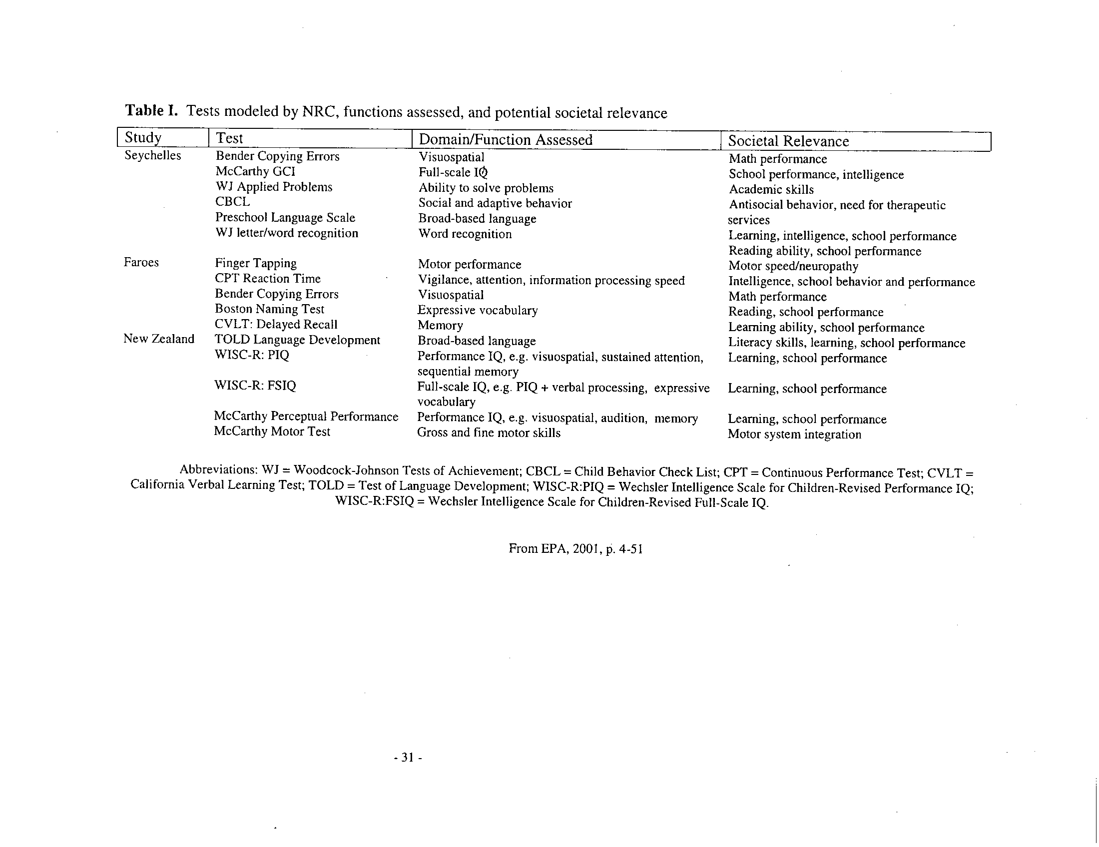
exposure and effect. The NRC modeled the relationship between maternal body burden and the

child's performance on five endpoints from the Faroe Islands study from a total of nine that had

been reported as significantly affected by methylmercury exposure (Grandjean et al., 1997)

(Table I). Similarly, five endpoints negatively associated with methylmercury exposure in the

New Zealand study (Kjellstrom et al., 1989) were used in the BMD analysis by the NRC . All of

the endpoints assessed in the Seychelles study were also modeled, even though the Seychelles

study was reported as negative . For the Faroe Islands study, maternal blood mercury

concentration was used as the exposure metric ; for the other two studies, only hair mercury

levels were available

.

In BMD analysis, the first step is to model the relationship between the endpoint

(neuropsychological performance) and exposure (body burden). The NRC used the K power

model, and determined the K value that best fit the data . The model was constrained to K >= 1

.

This allowed a sublinear relationship

:

i .e ., a lower slope at lower body burdens and a

comparatively greater slope at higher body burdens . The NRC reasoned that a supralinear model

was biologically implausible . Under these conditions, the best fit to the data was K=1, or a linear

dose-effect relationship, which was the model used for all endpoints from all three studies . In

fact, for the Faroe Islands endpoints, supralinear models such as the square root or logarithmic

transformations were a better fit than the linear model (Budtz-Jprgensen et al., 2000). In other

words, there was evidence that the slope was actually steeper at lower body burdens compared to

higher ones. This was also the case for the endpoints from the New Zealand study (Louise Ryan,

statistician on the NRC panel, personal communication) . This means that there was no evidence

of a threshold within the body burdens of these studies (range of 0.17-39.1 ppm in hair in the

Faroe Islands study [Grandjean

et al.,

2005]) .

Benchmark dose analysis requires two additional decisions once an appropriate model

has been chosen . When continuous data are used, a point on the curve below which responses

are considered "abnormal" must be chosen, termed P 0

. A value of PO = 0.05 was used in the

NRC assessment: that is, the cutoff for abnormal response was set at the lowest 5% (5th

percentile) of children. This is roughly comparable to an IQ of 75 in terms of population

distribution. The second decision that must be made is the choice of the increase in the

proportion of individuals that will be expected to perform in the "abnormal" category in an

exposed versus an unexposed population. This is defined as the benchmark response (BMR) . A

BMR of 0.05 was chosen for this assessment, which would result in a doubling of the number of

-

1 0

-

---

children with a response at or below the 5th percentile in an unexposed population. The lower

95% confidence limit on the BMD (BMDL) was determined for each endpoint

.

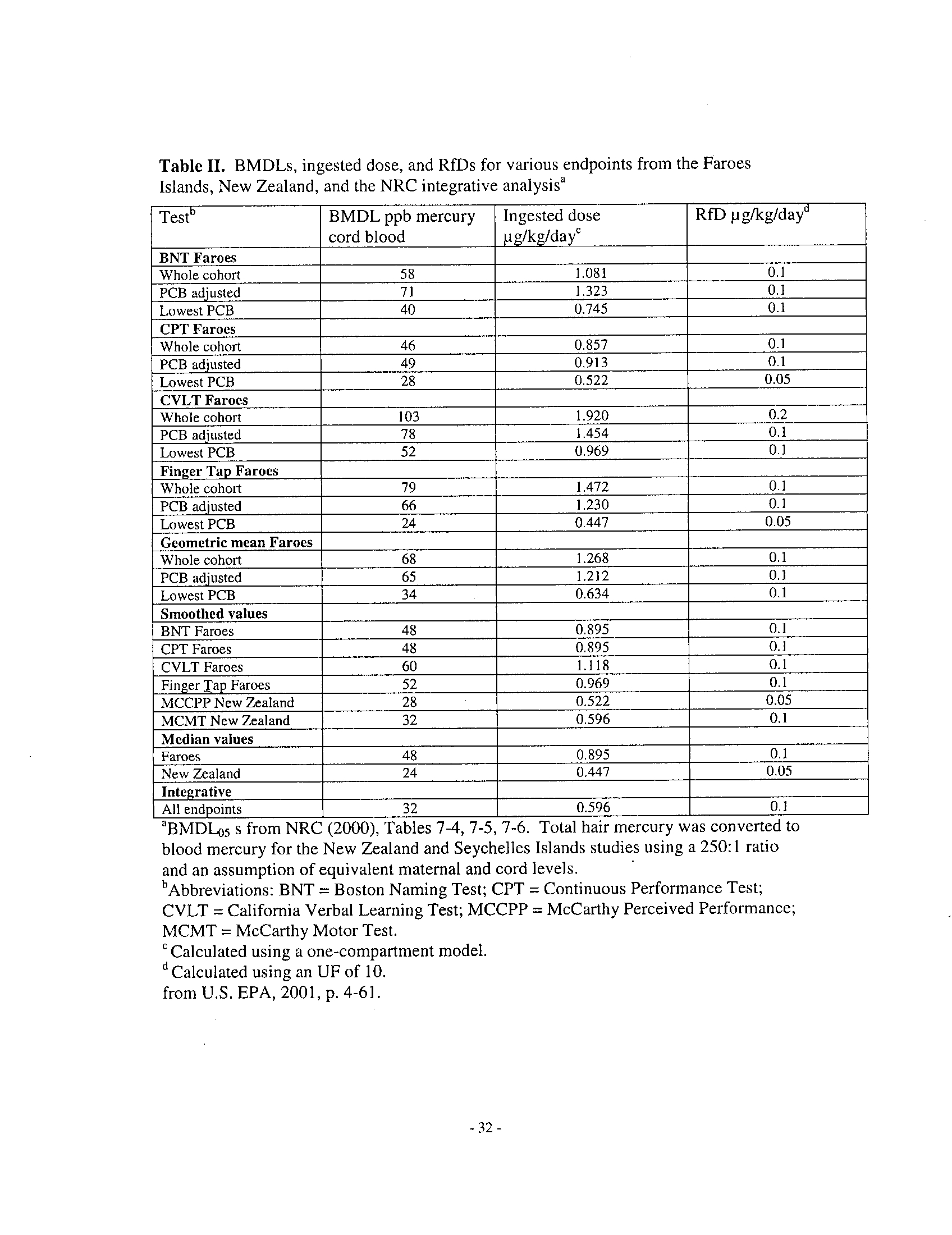
The BMDLs were highest for the Seychelles Islands study and lowest for the New

Zealand study (Table II). The NRC also performed a combined BMD analysis, using hair

methylmercury data from all three studies . The BMDLs from the Faroe Islands study were 12-15

ppm total mercury in maternal hair, whereas those in the New Zealand study were 4-6 ppm

.

BMDLs from the Seychelles Islands study were 17-25, about 50% higher than those in the Faroe

Islands and 250-300% higher than those from the New Zealand study . It is important to

recognize that the BMDL represents a defined risk level : in this case, a doubling of the number

of children performing in the abnormal range. It is therefore not equivalent to the NOAEL (no

observed adverse effect level), which be definition is a level at which no adverse effects are

identified

.

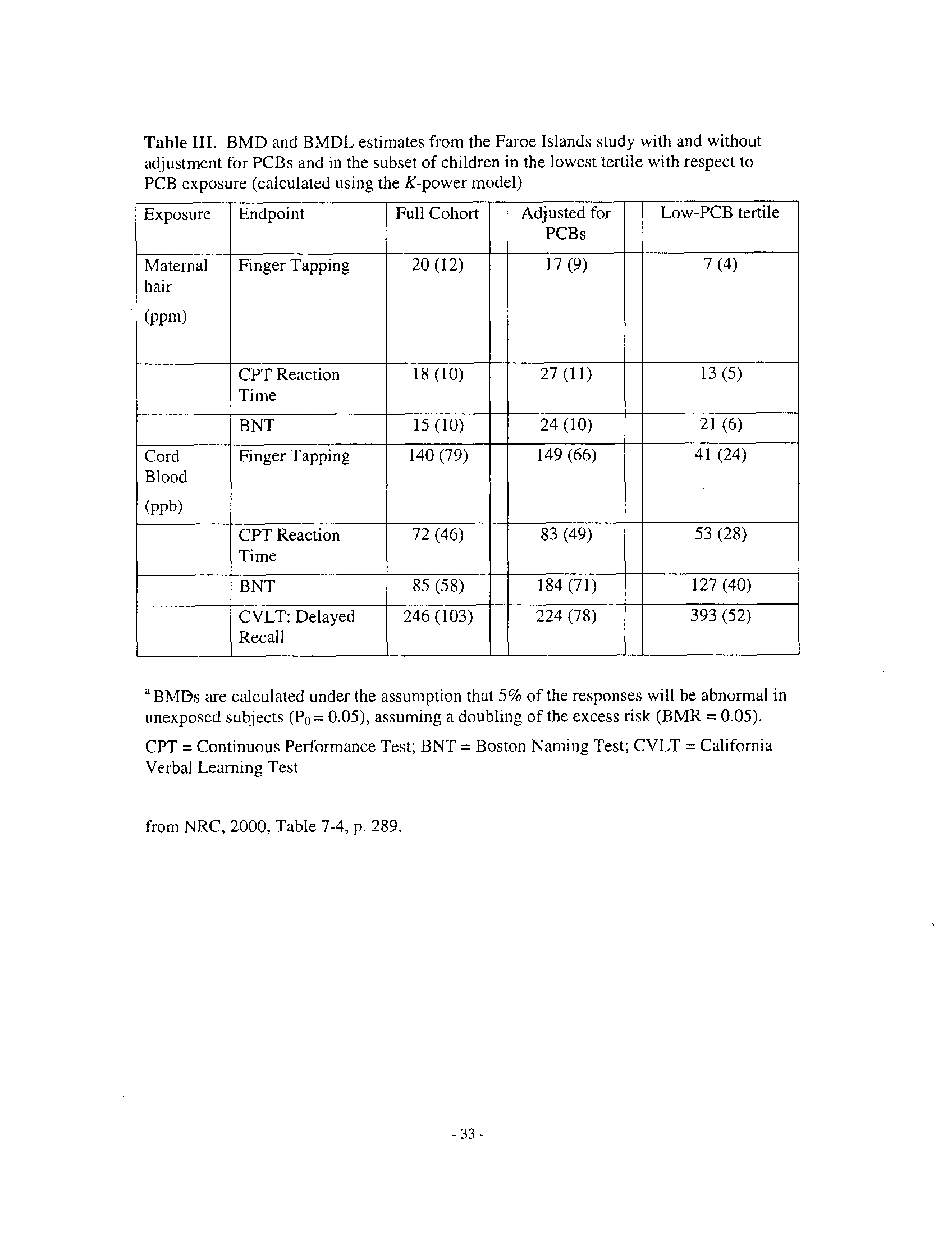
The NRC examined the issue of potential confounding by PCBs in the Faroe Islands

study in some detail. PCB body burden data were available for half the cohort (about 450

children). Analyses were performed controlling or not controlling for PCBs, with no systematic

effects on BMDLs (Table III) . Additional analyses were performed dividing the cohort into

tertiles with respect to PCB levels; again there was no evidence that higher PCB body burden

was related to a greater effect of methylmercury

.

The NRC believed that the negative Seychelles Islands study should not be used as the

basis for risk assessment, given the evidence of adverse effects found in the Faroe Islands and

New Zealand studies. The NRC recommended the Faroe Islands study as the study upon which

to base a hazard analysis for several reasons. First, the Faroe Island study is considerably larger

than the New Zealand study. In addition, this study has been ". .

. extensively analyzed and re-

analyzed to explore the possibility of confounding, outliers, differential sensitivity, and other

factors" (NRC, 2000, p. 299). The NRC recommended the cord blood concentration of 58 ug/L

associated-with the BMDL from the Boston Naming Test as a suitable basis for derivation of the

RfD .

Conversion of Cord Blood Concentration to Maternal Methylmercury Intake

Cord blood was a better predictor of performance than hair in the only study that used

both biomarkers (Faroe study), although maternal hair mercury was also associated with

decrements in performance in both the Faroe and New Zealand studies . Hair mercury represents

an integration of exposure throughout gestation if a sufficient length of hair is analyzed . Cord

blood mercury represents exposure more proximal to delivery. Hair represents an excretion

compartment more removed for the fetus than cord blood . The NRC stated that there was no

compelling evidence to consider one biomarker more appropriate than the other. The committee

recommended the use of cord blood because it explained

".

. . more of the variability in more of

the outcomes" (NRC, 2000, p . 286). In addition, modeling the association between cord blood

and maternal mercury intake is more straightforward than inclusion of a hair excretion

compartment

.

The U .S. EPA (2001) used a one-compartment pharmacokinetic (PK) model to estimate

the intake associated with BMDLs from a number of endpoints from both the Faroe Islands and

New Zealand studies, as well as the integrated analysis of all three studies . The EPA used

---

central tendencies for the parameters rather than estimating distributions . The EPA also assumed

that the ratio of cord :maternal blood mercury concentration was 1 .0, even though EPA

acknowledged that it was probably greater than one . The EPA applied a total uncertainty factor

(UF) of 10 below the BMDLs from the various endpoints modeled by the NAS (EPA, 2005 ; Rice

et al .,

2003) (Table II). It is unclear whether this OF provides sufficient protection against

adverse effects, given that there was no evidence of a threshold in the modeling performed by the

NRC, as well as new analyses regarding the pharmacokinetics

of

methylmercury

.

Since the EPA assessment, two important analyses have been published . A distributional

analysis

of

the cord:matemal blood ratio identified a central tendency of 1 .7, and a 90` h percentile

of 3.3 (Stern and Smith, 2003). Using the central tendency of 1 .7, 58 ug/L in cord blood would

be associated with 34 ug/L in maternal blood. For mother-fetal pairs at the 90 th percentile, a cord

blood level of 58 ug/L would be associated with a maternal blood level of about 18 ug/L

. These

are maternal blood levels associated with a doubling in the number of children performing in the

abnormal range on the Boston Naming Test of the Faroe Islands study

.

Stern subsequently performed a probabilistic (Monte Carlo) full distribution analysis of

the one-compartment PK model (Stern, 2005). The one-compartment model is preferable to a

physiologically based (PB) PK model because it requires fewer assumptions . In addition, the

one-compartment model provides a good predictor of the relationship between intake and blood

mercury levels under steady-state (chronic intake) conditions . Stem expanded the model used by

EPA (2001) to include the cord blood:maternal blood ratio

:

D_Cx(1/R)xbxV

WxAxF

where D = maternal intake of meHg (ug/kg)

C = mercury concentration in cord blood (58 ug/L)

R = ratio of cord:maternal blood (unitless)

b = rate constant of elimination from blood (day

-')

V = maternal blood volume (L)

W = maternal body weight (kg)

A = fraction of ingested dose that is absorbed (unitless)

F = fraction of absorbed dose in blood (unitless)

The BMDL value of 58 ug/L recommended by the NRC was used in the analysis

.

Distributions for each variable were chosen from the published literature, with preference given

to third-trimester data. Studies were chosen for which distributions were provided in the

publication under consideration or could be derived from the data provided in the paper. Results

were based on the average of five separate simulations of 5000 iterations each . Sensitivity

analyses of variability revealed that R made the biggest contribution to output variability,

followed by b, F, and W. V and A made no significant contribution to the variability .

Sensitivity analysis of central tendency suggested that uncertainty in the most uncertain input

parameters would likely influence the estimate of maternal dose by <= 20%

.

The analysis identified a mean intake of 0 .99 ug/kg/day and a median (50` h percentile) of

0.81 ug/kg/day associated with a cord blood concentration of 58 ug/L . The 5`h percentile was

-

1 2 -

---

0.30 ug/kg/day, and the V' percentile was 0 .20 ug/kg/day. In other words, for 1% of U.S .

women, an intake of 0.20 ug/kg/day would result in a cord blood mercury concentration of 58

ug/L. This is only a factor of two greater than the RfD, and may provide no safety factor against

risk for these mother-infant pairs

.

Behavioral effects in animals

Neuropathological effects of developmental exposure to methylmercury have been

characterized in humans, monkeys, and rodents (see reviews by Reuhl and Chang, 1979

;

Burbacher

et

al .,

1990a). There are both similarities and differences, with the pattern of damage

in the monkey being more like that of the human than is the pattern in the rodent . Nonetheless, in

all species, methylmercury exposure at high doses produces decreased brain size ; damage to

cortex, basal ganglia, and other brain areas ; loss of cells; disorganized cell layers; ectopic cells

;

and loss of myelin. Therefore animal models may provide important information regarding

mechanism of action of methylmercury toxicity, as well as characterization of functional deficits

.

Effects in monkeys

There is a substantial database documenting adverse effects produced by methylmercury

exposure in animals, particularly following developmental exposure (NAS, 2000 ; Newland and

Paletz, 2000; Rice, 1996a; Gilbert and Grant-Webster, 1995) . A significant body of research has

been performed in monkeys, for several reasons . The structure of the monkey brain is more

similar to that of the human than is the rodent brain . The rodent brain has a smooth

(lyssencephalic) cerebral cortex, whereas the cortex of the primate (including human) brain has a

highly convoluted surface (gyrencephalic brain). This difference is particularly important with

respect to the damage produced by methylmercury, which preferentially damages structures

within sulci. The kinetics of methylmercury in rodents is quite different from that in the primate

.

Methylmercury is bound to sulfur in red blood cells, and the ratio of red blood cells to plasma is

much higher in the rat than the primate. The ratio of methylmercury in the brain compared to the

blood is about 1 :10 in rodents, but between 2:1 and 5 :1 in primates (see Rice, 1996a) . The

monkey is capable of more complex behavior than the rodent. The visual system of the monkey

is virtually identical to that of the human, whereas the rodent system is quite different . This is

particularly important since visual deficits are a hallmark of methylmercury exposure. Finally,

episodes of human poisoning and the resulting recognition of the potentially devastating effects

of methylmercury encouraged research in the most appropriate species

.

Research on macaque monkeys was performed in two laboratories (University of

Washington and Health Canada), in which cohorts of monkeys were exposed

in utero

only,

in

utero

plus postnatally through adolescence, or beginning at birth through young adulthood (7

years). In all these studies, infants were separated from their mothers at birth and reared in a

primate nursery. In the studies in which monkeys were exposed prenatally, the mothers were

dosed until blood mercury levels were stable, before initiation of breeding, to mimic

environmental exposure in humans

.

Visual function was assessed in all cohorts using a behavioral procedure in which the

stimuli and experimental task were controlled by computer. Deficits in spatial visual function

were observed in all three cohorts (Burbacher

et

al., 2005; Rice, 1996a; Rice and Gilbert, 1982)

.

High frequency and low luminance vision were most affected . Assessment of temporal visual

function indicated remodeling of the visual system during development, with preferential

-

1 3 -

---

damage to small cells . Auditory function was assessed in monkeys exposed pre- plus postnatal or

postnatally only (Rice, 1998 ; Rice and Gilbert, 1992) . Individuals in the former cohort were

impaired in their ability to detect pure tones across a range of frequencies . The monkeys exposed

beginning at birth were impaired only at high or high and middle frequencies, with low

frequencies spared. The ability of the monkeys in these cohorts to detect a vibrating needle in

contact with the tip of the finger was also determined (Rice and Gilbert, 1995) . As in the other

assessments of sensory system function, the stimulus presentation was controlled by computer

.

The monkey's hand was held in position over the blunt needle, and the frequency and amplitude

of the vibration were precisely controlled . Monkeys in both cohorts exhibited impairment in their

ability to detect vibration over a range of frequencies, which probably resulted from central

rather than peripheral damage. Monkeys in both cohorts were also impaired on a fine motor task

during middle age (Rice, 1996b), presumably as a consequence of somatosensory impairment

(see section on delayed neurotoxicity)

.

Experiments in monkeys also provide evidence for cognitive impairment . Monkeys

exposed to methylmercury only during gestation were impaired on an object permanence task

during infancy (Burbacher

et al.,

1988). This task tested the infants' ability to realize that a

desired object placed behind a screen was still present, as measured by their reaching behind the

screen to retrieve it. Methylmercury-exposed infants took longer to learn the task, and were

retarded in the development of the skill of simple reaching for the object when it was in view

.

These same monkeys were also deficient on a series of visual recognition tasks (Gunderson

et

al .,

1986, 1988). In this task, the subject is shown a stimulus (usually a picture), and after a delay

the subject is shown the original stimulus and a novel one . A normal animal or human infant will

gaze longer at the novel stimulus, which is considered to be indicative of recognition memory

and is a reasonable predictor of later IQ . Methylmercury-exposed monkeys were impaired,

exhibiting a decreased percentage of time looking at the novel stimulus compared to controls

.

The results of this study could also be due to deficits in higher-order visual processing, however,

as discussed by Newland and Palentz (2000) . Deficits were also reported on this task in U .S

.

infants at low maternal body burdens (Oken

et al .,

2005). This cohort also behaved differently

than controls in a social situation, exhibiting increased nonsocial and passive behavior, and

decreased rough-and-tumble play but not quiet social interaction (Burbacher

et al .,

1990b) .

The effects of methylmercury have been assessed on performance on a fixed interval (FI)

schedule of reinforcement . On this schedule, a response after a certain period of time has elapsed

is reinforced with food . Even though only one response is required, the FI engenders a response

pattern characterized by a gradually accelerating rate of response terminating in reinforcement

.

One aspect of performance assessed by this schedule is the temporal control of behavior, which

may be considered a higher-order cognitive ('bxecutive') function . Monkeys exposed prenatally

only (Gilbert

et al .,

1996) or pre- plus postnatally (Rice, 1992) exhibited a different temporal

pattern of performance compared to controls

.

In a study in squirrel monkeys exposed prenatally (Newland

et al.,

1994), the effects of

methylmercury were determined on a complex learning task that required adaptive response to

changing environmental contingencies . In the concurrent random interval-random interval

schedule, responses were reinforced on each of two levers, with one delivering a reinforcement

for a response at a shorter interval than the other . A normal subject will apportion responses

accordingly (e.g . if one lever pays off four times as frequently as the other, the subject will

respond on it about four times as often) . After the monkey learned the task, the relative

-

1 4

-

---

frequencies of reinforcement opportunity between levers was changed . Control monkeys

followed these changes in schedule contingencies appropriately, whereas the exposed monkeys

did not. This learning deficit suggests that the methylmercury-exposed monkeys were insensitive

to changes in the rules of their environment

.

In contrast to these findings, methylmercury-treated monkeys were not impaired on other

learning tasks (Rice, 1996a ; Gilbert

et al .,

1993). This suggests that the effects of methylmercury

on cognition are not global in nature

.

The doses in the studies with macaque monkeys (10-50 ug/kg/day to mother and/or

offspring)

resulted in blood mercury levels above those expected in human environmental

exposure. The highest dose, the only dose administered in the studies of

in utero

only or

postnatal only exposure, resulted in peak blood mercury levels during infancy of 0.8-1 .2 ppm. In

the study of pre- plus postnatal exposure, doses of 10, 25, or 50 ug/kg/day were given to the

mother during pregnancy and the offspring from birth to 4 years of age . Unfortunately, only a

single infant was born in the lowest dose group ; the maternal blood level was 37 ug/L, and the

infants' blood at birth was 46 ug/L (Rice, 1989a) . The infant born at the 10 ug/kg/day dose was

as impaired as individuals at higher doses. The effects observed on sensory systems were robust,

although the monkeys appeared normal upon observation until middle age (see section on

delayed toxicity). A no-effect level was not identified. Testing on many of these endpoints

occurred years after cessation of dosing, indicating that the effects were permanent

.

Behavioral effects in rodents

Methylmercury-induced neurotoxicity in the adult rodent is manifested mostly as

impairment to motor systems. Methylmercury neurotoxicity as a result of developmental

exposure was identified in the mouse by Spyker

et al .

(1972), who reported retarded growth and

increased mortality in pups exposed

in utero,

with no obvious effect on motor function

.

Neurotoxicity was revealed when these mice were forced to swim, however, displayed as

abnormal.swimming movements and posture . A number of subsequent studies in rats or mice

exposed to high doses of methylmercury during several days of gestation demonstrated gross

neurological signs, changes in activity, or impairment on simple learning tasks, usually in

conjunction with decreased maternal or pup weight, or increased pup mortality (Reviewed by

Rice, 1996a) .

Methylmercury has been chosen as a model agent for the validation of various test

batteries and/or determination of inter-laboratory reliability because of its potent action as a

neurotoxic agent in humans . In a collaborative study involving six laboratories in the United

States, the effects of 2.0 or 6.0 mg/kg of methylmercury administered on gestational days 6-9

were studied on negative geotaxis, olfactory orientation, auditory startle habituation, activity,

activity following a pharmacological challenge, and a visual discrimination task (Buelke-Sam

et

al .,

1985) . Facilitation of auditory startle at the high dose of methylmercury was reliably

observed across laboratories, with inconsistent or minimal effects on activity, pharmacological

challenge, and the discrimination task, in the presence of overt signs such as decreased weight

gain and delayed developmental landmarks . Additional research with a different battery of tests

using a subset of the rats from the U .S. collaborative study revealed delayed righting and

swimming ontogeny and decreased activity (Vorhees, 1985). Impairment was also observed on

performance in a complex water maze, a task heavily dependent upon intact motor function

.

Most effects were observed only at the high dose .

-

1 5 -

---

In a collaborative study in Europe, dams were exposed to methylmercury in drinking

water during pregnancy and lactation . Delayed sexual maturity and impaired righting and

swimming ability were observed in the offspring (Suter and Schon, 1986) . Assessment of

complex learning measured by visual discrimination reversal and spatial delayed alternation

performance revealed increased response latencies and an increased incidence of failure to

respond during a trial, with no effect on accuracy of performance (Schreiner

et al .,

1986; Elsner,

1986) . In addition, the pattern of locomotor behavior in a complex activity monitor differed

between control and methylmercury-treated offspring, with treated rats exhibiting less behavioral

diversity. In a follow-up study involving five European laboratories, dams were exposed to

methylmercury in doses of 0.0025-5.0 mg/kg/day on days 6-9 of gestation (Elsner

et al.,

1988) .

This study in general confirmed results of the previous study with respect to the lack of effect on

accuracy of performance in the visual discrimination and delayed alternation tasks

.

Methylmercury-treated offspring exhibited delayed vaginal opening, impaired swimming

behavior, decreased locomotor activity, increased amplitude in auditory startle, and decreased

activity on a variety

of

endpoints in the learning tasks . Most effects were observed only at the

highest dose, while impaired swimming ability, increased auditory startle, and failure to respond

on a spatial alternation task were observed at 0 .5 mg/kg. Delayed vaginal opening was observed

at 0.025 mg/kg, the lowest dose at which an effect was observed

.

In another study in which methylmercury was used to validate a test battery, dams were

dosed on days 6-15 to doses of 1, 2, or 6 mg/kg of methylmercury (Goldey

et al .,

1994). No

effects were observed on T-maze alternation, locomotor activity, amplitude or habituation

of

auditory startle, observational assessment, or olfactory discrimination at the lowest two doses

.

(The highest dose was lethal .)

In a pair of studies specifically designed to be sensitive to the known effects of

methylmercury neurotoxicity in the rodent, rat dams were gavaged with methylmercury on days

6-9 of gestation at doses between 0 .005 and 0.50 mg/kg (Musch

et al .,

1978; Bornhausen

et al .,

1980). Offspring were impaired in their ability to perform on a DRH schedule of reinforcement,

in which a number of responses on a lever were required in a specified (short) period of time

.

Methylmercury-treated offspring performed normally when required to press a lever twice within

one second to be reinforced (DRH 2/1), but not when the response requirement was

incrementally increased to DRH 4/2 and then DRH 8/4 . Both male and female rats were reliably

affected at a dose of 0.01 mg/kg, the lowest dose at which effects have been observed in rodents

.

The robust effects observed on this paradigm may be the result of motor impairment, although

cognitive deficits also may have contributed to the poorer performance of the treated rats

.

Rats whose dams were exposed to 0 .5 or 1 .5 ppm methylmercury during gestation were

trained as adults to press a small platform with a force between two defined limits (Elsner, 1991)

.

The exposed rats were impaired on this task, which could reflect sensory and/or motor

impairment. These rats also displayed impaired swimming ability, which could also result from

both sensory and motor deficits . These results replicated previous findings (Elsner

et al .,

1988) .

Some individuals had tremors, clearly a motor effect

.

In a study of several aspects of behavior, mouse dams were exposed to 0, 4, 6, or 8 pm

methylmercury in drinking water during gestation and lactation (Goulet

et al.,

2003). Pups were

tested on rotorod (a test of gross motor function), spatial alternation (a test of working memory),

and locomotor activity. Working memory was impaired in females in the two highest dose

groups on one of two tests of working memory, and locomotor activity was decreased in females

- 16

-

---

in all groups . This study reported cognitive effects in mice in the absence of gross motor

impairment as measured by ability to stay on a rotating rod . Similar effects on working memory

were observed in a previous study by this group of investigators (Dore

et al., 2001) . .

In a study on the potential interaction of methylmercury and PCBs on behavior, rat dams

were exposed during pregnancy to 0 .5 ppm methylmercury in drinking water to postnatal day 16

(Widholm

et al., 2004) .

Offspring were tested on a spatial memory task (delayed spatial

alternation) beginning at 110 days of age. Methylmercury-exposed rats were impaired on this

task across all delay values, suggesting a cognitive deficit other than memory. There was not an

interaction between methylmercury and PCBs in this study

.

It is clear that the most salient effect of methyl mercury exposure in the rodent is

impairment of motor function, particularly on test batteries . Results of tests of cognitive function

were largely negative or showed a very weak high-dose effect . However, testing on more

sophisticated tasks revealed cognitive impairment . (See section on delayed neurotoxicity for

description of other studies in which cognitive impairment in rodents was reported .) Little

research has been performed in the rodent on the effects of methylmercury exposure on sensory

system function

.

In utero

exposure has been reported to result in changes in visual evoked

potentials (Zenick, 1976 ; Dyer

et al .,

1978). Goldey

et al .

(1994) found no effect on auditory

threshold for pure tones .

Evidence for long-term and delayed effects

Effects in animals

The possibility that methylmercury may produce toxicity during old age was recognized

early. Mice exposed to methylmercury

in utero

displayed abnormalities of various sorts as these

animals aged not present earlier, including kyphosis, obesity, apparent immune impairment, and

severe neuropsychological deficits (Spyker, 1975)

.

Evidence of delayed neurotoxicity as a result of developmental exposure to

methylmercury has also been observed in monkeys in the Health Canada laboratory . When the

group of monkeys exposed from birth to 7 years of age was 13 years old, it was noted

incidentally by animal care staff that some of these individuals appeared clumsy and hesitant in

the large exercise cages. This observation was considered to be particularly important in view of

the possibility that these signs represented methylmercury-induced delayed neurotoxicity

manifested many years after cessation of exposure . Observation of these monkeys in the large

cages in which they had exercised and socialized since infancy revealed clumsiness in some

treated individuals, a tendency for the hind feet to slip down the bars when climbing, and a

preference for climbing from area to area rather than jumping. Assessment by a veterinarian

revealed a higher incidence of failure to respond to a light touch or pin prick to the hands, feet, or

tail (Rice, 1996b). In a test of fine motor control, treated monkeys retrieved raisins from recessed

wells more slowly than controls, with some treated monkeys having difficulty removing the

raisins from deep compartments. These monkeys had undergone routine clinical assessment of

sensory and motor function from infancy to about four years of age, with no signs of toxicity

noted. The observation of overt toxicity at age 13, six years after cessation of dosing, therefore

represents delayed neurotoxicity as a consequence of methylmercury exposure . During old age,

some of these individuals had protruding tongues, which was considered indicative of perioral

hypoesthesia, a recognized effect of methylmercury poisoning . The group of monkeys exposed

in utero

to four years of age were also slower than controls to retrieve raisins from recessed

-

1 7

-

---

compartments, even though these monkeys were not overtly clumsy . While it was not possible to

rule out motor damage in these groups of monkeys, it seemed reasonable to assume that the

observed slowness and clumsiness was at least partly the result of somatosensory damage, based

on the results of these relatively crude assessment procedures . Objective assessment of

somatosensory function confirmed impairment in the ability of these monkeys to detect vibration

in the fingers. (See section on behavioral effects in animals .)

The ability to detect pure tones over a range of frequencies was examined at I 1 and 19

years of age in the group of monkeys exposed during gestation and continuing to four years of

age (Rice, 1998). At the first assessment, monkeys in the high-dose group were impaired at

higher frequencies, whereas at the second assessment, the high-dose group was impaired at more

frequencies relative to controls, and the lower-dose individuals were also impaired . This

represents delayed neurotoxicity for this functional domain, and demonstrates an interaction of

aging and previous methylmercury exposure in these monkeys . Visual function was also

reassessed in both cohorts of monkeys during old age (Rice and Hayward, 1999), and compared

to results from assessment at younger ages . Visual function declined in all animals as a result of

aging, with no differential effect produced by methylmercury. However, some treated individuals

displayed mild constriction of visual fields that had not been present when younger

. Constriction

of visual fields is a hallmark of high exposure to methylmercury in adults

.

The effect of methylmercury exposure was studied in mice exposed to 1 or 3 ppm

perinatally or over the lifetime (Weiss

et al .,

2005). Mice in all groups were impaired on landing

foot splay (an assessment of gross motor integrity), wheel running, and delayed alternation

.

There was an interaction between performance and age at testing, which was different for

different measures. These data provide additional evidence for the interaction of aging and

methylmercury exposure on neurotoxicity

.

Evidence for delayed neurotoxicity was documented in a study of rats exposed to

methylmercury during gestation and until postnatal day 16 (Newland and Rasmussen, 2000),

using the DRH schedule described above . This task requires a sustained motor response . Rats

were tested beginning at about 120 days old and continued until they were more than 900 days of

age. The rate of response declined in all groups, but declined at younger ages in methylmercury-

exposed groups in a dose-dependent manner . These results indicate an interaction of aging and

developmental methylmercury exposure

.

The effect of gestational and lactation exposure to methylmercury on performance of

aging rats was also explored in the concurrent random interval-random interval schedules of

reinforcement (Newland

et al .,

2004). Performance on this schedule was also assessed in

monkeys, described above. The rate of each rat's ability to adapt was measured by determining

how quickly the relative response rate changed following a change in the relative payoff on the

two levers. There was no difference on this measure or other measures of performance in 1

.7-

year-old rats whose mothers were exposed to 0 .5 or 6.4 ppm mercury in food. When their 2.3-

year-old littermates were tested at 2 .3 years of age, however, both groups of treated rats were

slower to make the transition . These results demonstrate failure to adapt to new environmental

contingencies (learning) in old rats exposed developmentally to methylmercury, but not in

younger ones .

Effects in humans

-

1 8 -

---

There is also evidence for delayed neurotoxicity as a result of methyhnercury exposure in

humans. It was recognized early that the onset of Minamata disease was delayed in some

individuals, by as long as several years, and that manifestations of disease became worse over

time in some cases (Igata

et al .,

1993; Tsubaki and Irukayama, 1977). Hundreds of cases were

diagnosed in Niigata years after the presumed cessation of ingestion of contaminated fish,

although some individuals may well have been ill before presenting themselves for diagnosis

.

Interestingly, the frequency of signs showed a different distribution compared to early-onset

Minamata disease (Tsubaki and Irukayama, 1977) : in particular, the lower incidence of

constriction of visual fields observed in `late onset" Minamata disease. In patients diagnosed

after 1974, the frequency was less than 5% . On the other hand, disturbances of somatosensory

function were present in almost every individual. This is consistent with the somatosensory

deficits observed in aging monkeys

.

An important study of 1144 patients over the age of 40 with Minamata disease,

representing over 90% of diagnosed patients, and an equal number of age and gender matched

controls, was undertaken to determine the functional ability of people with Minamata disease as

they aged (Kinjo

et al.,

1993). Subjects completed a questionnaire of subjective complaints and

ability to perform activities of daily living (ADLs) including eating, bathing, face washing,

dressing, and using the toilet . People with Minamata disease had higher rates of response than

controls in all 18 subjective complaints investigated in the study . Perhaps the most important

finding, however, was that for ADLs, the relative deficit between controls and people with

Minamata disease increased with increasing age in a statistically-significant manner . In other

words, the interference of Minamata disease with the individual's ability to perform the

necessities of daily life grew worse as the individual aged, even though exposure to

methylmercury had ceased 20-30 years previously. These findings represent concrete evidence of

`delayed neurotoxicity" in a human population as a result of exposure to an environmental

neurotoxicant .

Individuals exposed to methylmercury in the Japanese poisoning episode reported

paresthesias of the distal extremities 30 years after cessation of exposure (Ninomiya

et al.,

2005)

.

Increased touch thresholds were present in both proximal and distal extremities, as were two-

point discrimination thresholds in forefingers and lips of 3 MD individuals . Similar effects were

also found in 32 persons exposed to methylmercury but not officially diagnosed as having MD

.

Median hair mercury levels in the group not diagnosed with MD was 37 ppm in 1960, and 2 .4 at

the time of testing (the hair mercury levels of the control group was 2 .8)

. For the group with MD,

hair levels in 1960 were 39-65 ppm. Results were interpreted as indicative of damage to

somatosensory cortex. This was also suggested as the underlying damage responsible for

somatosensory deficits in the monkey studies (Rice, 1996b) . A similar study of individuals with

Minamata Disease 60-79 years of age assessed ability to detect abrasive papers of various grits

(Takaoka

et al .,

2004). Subjects included individuals with MD, a group from Minamata without

numbness who were not diagnosed with MD, and a control group from another area . The ability

to detect whether pairs of papers were different (difference threshold) was determined . The MD

group had the biggest difference thresholds, and the group from Minamata without MD also had

greater difference thresholds than controls . Many of the MD group also had other signs of MD,

including ataxia and constriction of visual fields . Hair mercury levels were 2.8 ppm in controls

60-79, and 2 .4 ppm in MD individuals. These studies do not definitively document delayed

neurotoxicity, since it is unknown whether these individuals were impaired in the 1960s

.

-

1 9 -

---

Nonetheless, it is clear that exposure to methylmercury four decades before evaluation resulted

in permanent impairment

.

Although

the molecular mechanisms of delayed neurotoxicity remain unknown, there are

a number of relatively obvious ways in

which

toxicity could continue to be expressed or even

exacerbated (and which are not mutually exclusive) : 1) mercury stores in the body, specifically

in the nervous system, continue to exert a toxic influence, 2) damaged neurons or other nervous

system cell types may die prematurely, or 3) normal cells, required to compensate for damaged

or missing cells, may undergo accelerated aging. There are at least limited data relevant to the

first suggestion . Approximately 8 months after cessation of chronic dosing with methylmercury

in the monkey, and months after blood mercury levels decreased below the detection level, brain

contained significant amounts of total mercury (Rice, 1989b) . In a study examining speciation of

mercury after chronic methylmercury exposure in the monkey (Vahter

et al.,

1994, 1995), the

proportion of inorganic mercury increased with duration of exposure, and was

highest

if a period

of several months elapsed between cessation of exposure and autopsy . In fact, inorganic mercury

levels remained relatively constant whereas methylmercury levels decreased drastically . These

data suggest that the half-life of mercury in the brain is longer than in blood after methylmercury

exposure, and that this is at least in part the result of conversion to inorganic mercury in brain

.

Inorganic mercury was concentrated in astrocyte and reactive glia following chronic low-level

methylmercury or inorganic mercury exposure in the monkey (Charleston

et al .,

1994, 1995) .

The authors suggest that these astrocytes and possibly microglia are the primary sources of

demethylation of methylmercury . Astrocyte and/or microglia cell numbers decreased in various

brain areas following methylmercury exposure in the absence of changes in neuronal cell

numbers (Charleston

et al .,

1994, 1995, 1996) . The authors suggest that this may represent the

proximal cause of neurotoxicity,

although

the degree to which these findings would extrapolate

to lower exposures is unknown. The long-term consequences of methylmercury exposure in

adults in Minamata is consistent with results from the monkey studies

.

Mechanisms of toxicity

It is very clear from the episodes of human poisoning that the fetus and infant were more

sensitive to the effects of methylmercury than the adult, and that effects were qualitatively as

well as quantitatively different . In both the adult and developing organisms, methylmercury is

found

throughout

the brain, so that differential distribution probably does not account for the

different pattern of pathology

.

The brain develops by a series of processes that are exquisitely choreographed both

spatially and temporally. Most of these processes are unique to the developing brain ; therefore

toxicants can affect the developing brain in ways not possible in the adult brain . These processes

include neurogenesis and proliferation, migration of neurons from their origin to their final

locations in the brain, differentiation of the immature neurons to their final cell type, the

formation of synapses (connections) between cells and thereby between brain areas, birth and

differentiation of numerous supportive cell types responsible for maintenance of normal brain

development and function, myelination (the wrapping of nerve processes in a protective

sheath

that increases the speed to communication between nerve cells), and apoptosis (the genetically-

programmed death of cells and pruning of connections that is vital to normal brain functioning) .

All of these processes are affected by methylmercury exposure (Rice and Barone, 2000) .

- 20

-

---

The control of brain development is orchestrated by a large assortment of molecules

(signal transducers) that regulate the integration of genetic and epigenetic events . The effects of

methylmercury on many of these systems has been investigated, and the mechanisms of

methylmercury neurotoxicity are well characterized (Aschner and Syversen, 2005) . Some of

these mechanisms are relevant to adults, whereas others are particularly important during

development .

An important mechanism is inhibition of glutamate uptake, and stimulation of its efflux,

resulting in excitotoxic injury . Methylmercury inhibits uptake systems for cystine and cystine

transport, compromising glutathione synthesis . This would result in increased susceptibility to

reactive oxygen species (ROS). ROS are known to mediate methylmercury-induced

neurotoxicity in a variety of experimental models . There has also been a substantial amount of

research on the cascade of events leading to glutamate neurotoxicity produced by

methylmercury

.

The ability of methylmercury to interfere with neuronal migration, a salient feature of

developmental methylmercury poisoning, is undoubtedly the result of interference with various

microtubular elements, including N-CAM, astrotaction, and LI (Aschner and Syversen, 2005)

.

Methylmercury also interferes with mitosis (Rodier

et al.,

1984), which would inhibit cell

proliferation. It may be the case that at lower levels of exposure, inhibition of growth cone

outgrowth, leading to decreased axonal and dendritic development, plays an important role in

developmental neurotoxicity. Despite the relatively robust literature on the mechanisms of

methylmercury-induced neurotoxicity, the reasons for differential pattern of neuropathological

damage in the adult and developing brain are not understood

.

Cardiovascular Effects

Studies in adults

There is evidence from several studies that increased methylmercury body burden is

associated-with cardiovascular or coronary disease, including heart attack and stroke . The

potential for methylmercury to produce cardiovascular (CV) and coronary disease was identified

as an important concern (EPA, 2001) that requires further analysis . Studies have identified

effects at hair mercury levels within the range of exposures in the U .S. The relatively sensitivity

of CV versus developmental neurotoxic effects is unknown, since the required dose-effect

modeling has not bee performed for CV effects . The evidence has been recently reviewed (Stern,

2005) .

In a study of 2500 men in Finland, acute myocardial infarction (AMI) and fatal coronary

events were followed for an average of 6 years (Salonen

et al .,

1995). Hair samples for mercury

analysis and dietary data were obtained at the beginning of the study. The estimated mean dietary

intake of methylmercury was 7 .6 ug/day, about the same as that corresponding to the EPA

reference dose of 7 .0 ug/day for a 70 kg man . Mean hair mercury concentration was 1 .9 ppm .

Hair concentrations in the upper tertile (2 ppm) were associated with increased myocardial

infarction (MI) (relative risk =

1 .6) . There were non-statistically significant associations between

hair mercury concentration and death from coronary heart or CV disease. Fish intake of 30 g/day

was also associated with these outcomes . A follow-up study (Rissanen

et al .,

2000) examined the

effects of methylmercury and omega-3 fatty acids on these same endpoints, the latter of which is

believed to be protective against coronary disease. An interaction of serum omega-3 fatty acids

(DHA + DPA) and methylmercury in hair was found . Men with hair mercury levels above 2 ppm

- 2 1 -

---

received less benefit from omega-3 fatty acids than those with lower levels, with no reduction in

risk at all across the upper three quintiles of omega-3 fatty acid blood levels . This suggests that

higher body burdens of methylmercury may negate the protective effects of fish oils . A further

follow-up in this cohort was performed in 1871 men 42-60 years of age an average of 13

.9 years

after study initiation (Virtanen

et al.,

2005). Men with the highest tertile of hair mercury levels

were at significantly increased risk for acute coronary event (1 .60-fold; CI, 1 .24-2.06), CV

disease (1 .68-fold; CI, 1 .05-2.44), CHD (1.56-fold ; CI, 0.99-2.40), and any death (1 .38-fold; CI,

1 .15-1 .66) compared with men in the lower two tertiles . As in the previous study, high hair

mercury attenuated the beneficial effects of omega-3 fatty acids .

A study was performed by the same group of investigators on the progression of

atherosclerosis in 1014 men from eastern Finland (Salonen

et al.,

2000). This group was a subset

of those studied by Salonen

et al .

(1995). The relationship between thickness of the carotid

arteries and hair mercury was determined in 1014 men with an average age of 51

.9 years during

initial assessment, with a second measurement made 4 years later . The upper quintile of hair

mercury was 2.8 ppm. The relationship between hair mercury and increase in carotid wall

thickness was highly significant in a multivariate model ; in fact, the mercury effect was second

only to that for systolic blood pressure. There was no apparent effect across the first four

quintiles, with significant thickening in men in the highest quintile, suggesting a threshold for

this effect. In their earlier study, Salonen

et al .

reported an association between hair mercury

concentrations and immune titers to oxidized low-density lipids (LDL), suggesting a mechanism

for the association between mercury levels and atherosclerosis in this study

.

A multicenter case-control study was performed in a total of 1408 men 70 years old or

younger in eight European countries and Israel (Guallar

et al .,

2002). Cases were defined as men

hospitalized with a first MI, and age-matched controls were selected for the same geographical

areas as cases . Mercury exposure was determined from toenail clippings, and DHA was

determined in subcutaneous fat. After covariate adjustment, the mercury concentration in cases

was significantly higher than in controls . After adjustment for center, age, DHA, cardiovascular

risk factors, and antioxidants, the odds ratio (OR) was 2 .16 (CI, 1 .09-4.29) for the upper quintile

compared to the lowest quintile . As in the Rissanen

et al .

(2000) study, the results suggest that

mercury antagonized the protective effect of omega-3 fatty acids . Toenail mercury is a non-

standard marker of exposure. Further, it is unknown to what extent inorganic mercury exposure

may have contributed to toenail mercury levels . However, there was a reasonable

correspondence between mercury and DHA levels (r = .34) ;this suggests that the main source of

mercury was methylmercury from fish, since the main source of DHA would also presumably be

fish .

A nested case-control study of the effects of mercury exposure on coronary heart disease

(CHD) was conducted in U.S. male health professionals who were 40-75 years old at recruitment

(Yoshizawa

et al .,

2002). Each of 470 cases was matched with a control for age, smoking status,

and time of sampling. Toenail mercury was higher than in the Guallar study, with the dentists

having twice the mercury levels of other participants . This was presumably the result of exposure

to mercury vapor in their dental practice . After adjusting for risk factors, mercury levels were not

associated with risk of CHD. When dentists were eliminated from the analysis, a relative risk

(RR) of 1 .27 was found. After further adjustment for DHA and EPA levels, the RR was 1 .70 .

These were not statistically significant, which may be a consequence of reduced statistical

- 22

-

---

power. These results suggest that it is methylmercury that is responsible for CV risk, rather than

total mercury or inorganic mercury .

A small case-control study for first-time myocardial infarction (MI) including both men

and women was performed in Sweden (Hallgren

et

al .,

2001). A total of 78 cases and an equal

number of controls matched for sex, age, and geographical region were recruited over a 10-year

period. Blood samples were presumably collected at recruitment, as much as 10 years before the

MI. Mercury was measured in erythrocytes, and EPA and DHA were measured in blood plasma

.

The omega-3 fatty acid concentrations were associated with decreased risk, whereas there was no

effect of mercury concentration . The lack of effect may have been the result of low power,

although the study was of sufficient size to detect the beneficial effects of omega-3 fatty acids

. It

may also be the result of the inclusion of women, who may respond differently than men . The

OR for the low-fatty-acid - high-mercury group was greater than 1 .0, but consisted of only four

cases .

The relationship between blood pressure and blood mercury concentration was

determined in women 16-49 years of age in the NHANES (Vupputuri

et

al., 2005). There was no

overall relationship between mercury levels and blood pressure . However, when women were

stratified by fish consumption, there was an interaction between fish consumption and mercury

levels on blood pressure. In women who had not eaten fish in the last 30 days, there was an

increase in blood pressure as a function of increasing mercury quintile . For every 1 .3 ug/L

(interquartile range) increase in mercury level, there was a covariate-adjusted 1

.83 mm mercury

increase in systolic blood pressure, and a 0 .61 mm mercury (nonsignificant) increase in diastolic

blood pressure. This relationship did not hold among individuals who had eaten fish in the last

30 days. The authors postulated that omega-3 fatty acids in fish were protective . However, the

results are puzzling since fish was presumably the source of mercury in all women . The authors

did not have fatty acid levels in the women, nor did they try to estimate intake from the fish

species consumed . Perhaps the beneficial effects of omega-3 fatty acids were of shorter duration

than the deleterious effects of methylmercury. The average half-life in blood for methylmercury

is about 50 days, so that blood mercury levels represent fish intake as long as several months

previously

.

Studies in children

The Faroe Island investigators examined the relationship between methylmercury

exposure and blood pressure and heart rate at 7 and 14 years of age . At 7 years, systolic and

diastolic blood pressure, heart rate, and heart rate variability were assessed with respect to

in

utero

methylmercury exposure (Sorenson

et

al.,

1999). Cord blood mercury concentration was

significantly associated with increased systolic and diastolic pressure after control for covariates,

whereas maternal hair mercury was a poorer predictor. Blood pressure increased linearly as a

function of log cord blood from I to 10 ug/L, and did not increase thereafter. The effect was

greater in babies with birth weights below the mean (20 .9 and 20.4 mm mercury for systolic and

diastolic blood pressure, respectively, compared to 14 .6 and 13.9 mm for the group as a whole)

.

There was no effect on heart rate

per se,

but cord blood mercury was associated with decrease in

heart rate variability. In boys, there was a 47% decrease in heart rate variability as cord blood

increased from I to 10 ug/L. This was interpreted as indicative of action on the parasympathetic

nervous system producing effects on both blood pressure and heart rate variability

.

- 23 -

---

When the Faroe Islands cohort was reassessed at 14 years of age, associations between

blood pressure and heart rate with cord blood and children's hair mercury concentrations at 7 and

14 years were determined (Grandjean

et al .,

2004). At this later age, there were no associations

between methylmercury exposure and blood pressure . Cord blood mercury concentration was

associated with several parameters of decreased heart rate variability . The child's hair mercury

level at 14 years was associated with one measure of variability at 14 years, which decreased

after control for results at 7 years . The change was greatest at cord blood concentrations between

about I and 10 ug/L . The interpretation of these findings for public health is not entirely clear

.

Decreased heart rate variability in adults following an MI predicts sudden cardiac death

;

however, the applicability of these findings to other adults or children is unknown. On the other

hand, it is indicative of an effect on control of the autonomic nervous system, and therefore

provides additional evidence for an effect of methylmercury on nervous system function in this

cohort .

Animal studies

There are limited experimental data on the effects of methylmercury on CV function

. In a

study in adult rats, doses that did not produce gross toxicity produced increased systolic blood

pressure, which persisted throughout a 9-month post-dosing observation period (Wakita

et al.,

1987). Blood pressure increased as much as 30 mm mercury. Tamashiro

et al.

(1986) exposed

male and female spontaneously hypertensive rats to methylmercury for 26 days beginning at 7

weeks of age, at doses that produced overt toxicity. Blood pressure in females increased by about

20 mm mercury ; all males died soon after cessation of dosing . In an

in vitro

study, inhibition of

thrombin-mediated platelet aggregation by human umbilical vascular endothelial cells was

reversed in a dose-dependent manner by methylmercury Cl (Ohno

et al .,

1995). The authors

suggest that this effect is mediated through inhibition of endothelium-derived relaxing factor,

and suggests a mechanism for the effects of methylmercury on both vascular tension and

atherosclerosis observed in human studies .

Summary

Overall, there is reasonable support for an association between methylmercury exposure

and effects on CV function, including AMI. The study of Yoshizawa

et al. (2002),

which failed

to find an association in primary analyses, was flawed by the inclusion of a large percentage of

men exposed to mercury vapor in the control group . As discussed by Stern (2005), there is

substantial opportunity for exposure misclassification in these studies, since mercury body

burden may have changed substantially between exposure assessment and adverse event

. Since

this would bias results toward the null, the fact that studies identified associations provide

evidence for a reasonably strong effect. The potential for prenatal exposure to methylmercury to

contribute to later CV disease is unknown, but any such contribution could represent an

important societal burden from methylmercury exposure

.

Methylmercury levels in the U.S., and comparison to mercury levels associated with health

effects

The cord blood level corresponding to U.S. EPA reference dose is 5 .8 ug/L. However, the

maternal blood level associated with a cord blood level of 5 .8 ug/L is 3.4 ug/L, based on the fact

that cord blood is 1 .7 times higher than maternal blood, on average . The hair mercury level

associated with 3 .4 ug/L is about 0.65 ppm. Studies on the body burden of mercury in

individuals in the U .S. have used different values as representing elevated exposure, which is

- 24

-

---

reflected in the studies of body burdens of mercury in the U .S. discussed below. In addition, the

prospective study of the effect of methylmercu y on behavior of infants in the U

.S. dichotomized

data as above or below 1 .2 ppm maternal hair mercury in ancillary analyses

.

Blood and urinary mercury levels are analyzed as part of the NHANES (CDC, 2005)

.

Blood levels for 1999-2002 are available for children 1-5, females and males 16 and over, and

females 16-49 years. For children, the median blood mercury level was 0 .3 ug/L, with a 95` h

percentile of 2.3 (1999-2000) or 1 .9 (2001-2002) ug/L. For women of childbearing age, the

median was 1 .02 and 0.83 ug/L for the two time periods, with 95' h percentiles of 7 .10 and 4.60

ug/L. The 95`h percentile would correspond to hair mercury levels of approximately 1 .3 or 0 .9

ppm for the two time periods . Approximately 15 .7% of women of childbearing age had total

blood mercury levels >= 3 .5 ug/L (Mahaffey

et al .,

2004) in 1999-2000. For individuals who eat

fish more than three times a week

, the 95`h percentile hair mercury was 2 .00 ppm for children 1-

5 years old, and 2.75 ppm for women of childbearing age in 1999-2000 (McDowell

et al .,

2004) .

Using the NHANES database, hair mercury levels were examined for various ethnic

groups, including `other" (Asians, Pacific Islanders, Native Americans, and multiracial) women

of childbearing age (Hightower

et al.,

2006). The percentage of women with blood mercury

levels greater than 5.8 ug/L, as well as above 3 .5 ug/L, were determined. For whites, 11 % were

above 3 .5 ug/L, and 5.8% were above 5.8 ug/L. For `other" races, 27% were above 3 .5 ug/L,

and 16.6% above 5 .8 ug/L. These ethnic groups ate twice as many fish meals as whites or blacks,

and three times as many as Mexican Americans

.

The NHANES survey is designed to be representative of the U .S. population. However,

this survey does not adequately sample high-end fish consumers . In a survey of volunteers from

a random-dial survey of women of childbearing age in 12 states, mean hair mercury levels varied

between states from 0.21 to 1

.23 ppm, with higher levels in coastal states (Knobeloch

et al.,

2005). Fifty percent of women in NJ had hair levels above 1 ppm, as did 41% of women in CT

.

The 95`h percentile for all women who had eaten 20 fish meals in the last month was 2 .29 ppm,

whereas it-was 0.19 ppm for women who had not eaten fish. In a study of pregnant women

recruited through obstetric practices in NJ, about 10% had hair mercury levels above I ppm, with

about 1% above 6 ppm (Stern

et al.,

2001). Increased mercury levels were associated with

increased fish intake .

A recent survey of volunteers recruited through environmental organizations reported

hair mercury levels in 6503 individuals collected in 2004 and 2005, and the association between

hair mercury concentrations and fish intake (Environmental Quality Institute, 2005) . Children

less than 1 year old had median hair mercury levels of 0 .29 (girls) and 0.17 (boys) ppm, with 7 .7

percent of girls having hair mercury levels greater than 1 .0 ppm. For women of childbearing age,

the median was 0 .43 ppm, with 22.6% having hair levels above I ppm . Individuals over 50 also

had a substantial percentage of people with hair mercury levels above 1 ppm (24 and 29% for

females and males, respectively) . Hair mercury levels were associated with higher tuna fish and

total fish consumption, but not with dental amalgams . Since this was a self-selected population,

the distribution of levels presumably is not representative of the U

.S. population as a whole

.

Nonetheless, the study provides further evidence of a strong association between fish

consumption, including canned tuna, and increased methylmercury body burden. The study also

documents that at least for some populations, a substantial percentage of individuals have

methylmercury body burdens greater than that associated with the RfD

.

- 25

-

---

In a study in high-end fish consumers in a private medical practice, blood mercury levels

ranged from 2.0 to 89.5 ug/L for 89 individuals (Hightower and Moore, 2003) . Mercury levels of

7 children were determined in hair or blood, with the highest levels being 14 .8 ug/g in hair for a

7-year-old, above the BMD from the Faroe Islands study for defined effects .

The average exposures in the three large longitudinal studies of neuropsychological

effects in children were similar, based on maternal hair mercury concentrations . The geometric

mean in the Faroe Islands study was 4.3 ppm (interquartile range 2 .6-7.7 ppm), and in the

Seychelles Islands study the median was 5 .9 ppm (interquartile range 6 .0 ppm). In the New

Zealand study, the 'high" exposure group were women with >6 ppm, and these were matched

with three times as many children whose mothers had lower hair levels . The average exposures

in these studies are higher than those observed in the U .S. However, the ranges overlap those of

U .S. women. For example, the cord blood range in the Faroe Islands study was 0 .90-351 ug/L,

which would correspond to a maternal blood mercury level of 0 .52-203 ug/L based on an

average cord:maternal blood ratio of 1 .7. The Faroe Islands population clearly includes women

with higher exposures than those in the U .S ., but the range overlaps that of U .S. women. There

is no evidence for a threshold for adverse effects within the range of exposures in the Faroe

Islands. In the recent MA study that documented adverse effects (Oken

et al .,

2005), the mean

maternal hair mercury was 0 .55 ppm and the 90`h percentile was 1.2 ppm. This would

correspond to approximately maternal blood levels of 2 .7 ug/L and 5.8 ug/L, respectively. The

study by Jedrychowski

et al .

(2006) identified a significantly increased risk for developmental

delay on the Bayley Scales of Infant Development at one-tenth the RID, and at less than the

median of blood mercury levels of women child-bearing age in the U .S. Therefore it appears that

effects of exposure to methylmercury are present within the range of body burdens of U .S

.

women .

The body burdens of men in the studies on CV function and heart disease also overlap

those in the U .S. The mean hair mercury concentration in the Salonen

et al .

(1995), Risanen

et

al .,

(2000)', and Virtanen

et al .

(2005) studies of about 2 ppm is equivalent to about the 95

th

percentile for women in NHANES (corresponding data for men are not available, but mercury

levels are probably higher) . This level was associated with an increased risk of adverse CV

events, including MI . In the Yoshizawa

et al .

(2002) study, mean toenail mercury concentration

in non-dentists was 0.45 ppm, which presumably represents levels in the U .S. The toenail

mercury level associated with the highest quintile of exposure in the Guallar

et al .

(2002) study

was 0.7 ppm, suggesting that exposures in that study, in which increased risk of MI was

observed, is not much, if at all, different than exposures in the U .S .

Estimation of societal costs associated with methylmercury exposure in the U .S .

Of considerable importance is a recent analysis performed by Dr . Louise Ryan for the

U.S. EPA of all three longitudinal studies reporting that, in fact, the results from the three studies

modeled by the NRC are not discordant with respect to effects on IQ (Ryan, 2005

; EPA, 2005)

.

Ryan (2005) modeled results for IQ from the WISC-R at 6 years from the New Zealand study

and the WISC-I11 at 9 years from the Seychelles study. The Faroe Islands study did not assess

full-scale IQ at 7 years, but did measure performance on three subtests of WISC-R : Digit Spans,

Similarities, and Block Design . These measures were combined using structural equations

modeling (Budtz-JOrgensen

et al .,

2002). Bellinger (2005) points out that the correlation between

full-scale IQ and results on Similarities plus Block Design is 0.885. Adding the third subtest,

- 26

-

---

Digit Span, would presumably increase the correlation . This provides reassurance that combining

the scores on these subtests is a valid estimate of full-scale IQ . The relationship between

mercury hair levels and full-scale IQ was estimated for each study individually, and an

integrative analysis was performed combining all three studies. For each I ppm increase in

maternal hair mercury from I to 10 ppm, IQ in the offspring decreased by 0.13, 0.13, and 0.12

point for the New Zealand, Seychelles, and Faroe Islands studies, respectively . The integrative

analysis of all three studies yielded a decrement of 0 .13 IQ point for every 1 ppm increase in

maternal hair mercury . This analysis provides evidence that the three longitudinal studies are in

fact concordant with respect to effects on IQ . The Ryan/EPA analysis also modeled other

functional domains from the three studies in addition to IQ, and found concordance for multiple

domains

.

A quantitative risk-benefit analysis was performed by the Harvard Center for Risk

Analysis of changes in fish consumption in the U .S. population for several hypothetical

scenarios. This exercise, sponsored by the fishing industry, focused on the potential benefits of

omega-3 fatty acids on coronary heart disease (Konig

et al.,

2005), stroke (Bouzen

et al.,

2005),

and cognitive development. The authors of the paper addressing heart disease did not include

potential risks from methylmercury exposure . Four of the five authors of the paper on the

benefits of omega-3 fatty acids (Cohen

et al.,

2005a) also analyzed the risks of methylmercury

exposure in a separate paper (Cohen

et al .,

2005b). For the effects of mercury, the authors relied

on the analyses of the three studies by the NRC. The various domains were weighted in the

analysis, with a value of 1 .0 to tests of general intelligence, 0 .6 to language and

learning/achievement, 0.3 for attention, and 0.2 for motor. In addition, each study was weighted

on the basis of sample size and various considerations of the quality of each study . The weights

were 1 .0, 0.88, and 0.16 for the Faroe Islands, Seychelles, and New Zealand studies,

respectively. All analyses were integrated into an overall risk-benefit analysis (Cohen

et al .,

2005c). Scenarios for changes in fish consumption for women of childbearing age included (1)

elimination of fish with "medium" and "high" mercury levels (defined as >= 0 .14 ppm) and

substitution of an equal amount of "low" mercury fish, (2) a decrease of total fish consumption

by 17%, or (3) an increase of fish consumption by 50% without changing the species consumed

.

Under all scenarios, the loss of IQ associated with methylmercury intake was greater than the

gain conferred by consumption of omega-3 fatty acids. Under the first scenario, the net quality-

adjusted life years (QALYs) for methylmercury increased by 45,000, and for DHA 4,700 . Under

the second scenario, the methylmercury benefit was 17,000 QALYs, and the lost for DHA was -

5,800, for a net gain of 11,000. Under the final scneario, nondiscriminate increase in fish intake,

the methylmercury impact was -49,000, and the DHA benefit was 17,000, for a net loss of -

32,000 QALYs

.

Trasande

et al .

(2005) used data from the Faroe Islands study to estimate the cost

associated with exposure to methylmercury, based on IQ loss in children. They considered a cord

blood level of 5 .8 ug/L to be that associated with no impairment, based on data from the Faroe

Islands. A maternal blood mercury level of 4 .84 ug/L was considered to be associated with this

cord blood level using the cord :maternal blood ratio found in the Faroe Islands . A doubling in

blood mercury concentration above 4 .84 ug/L in maternal blood was considered to be associated

with loss of 0.85 to 2.4 IQ points. A number of factors were varied in a sensitivity analysis . A 1

.

ug/L increase in hair mercury concentration was considered to be associated with a loss of 0.59

to 1 .24 IQ points, and cord:maternal blood ratio was varied from 1 :1 to 1 .7 :1 . The upper bound

- 27

-

---

estimate assumed that children born to women with blood mercury levels of 3

.5-4.84 ug/L suffer

no loss in IQ, and the lower bound estimate assumed that children born to women with mercury

concentrations of 4 .84-5.8 ug/L suffer no loss in IQ. Using data on the association between IQ

and lifetime earnings, the cost of the loss of IQ produced by methylmercury exposure was

estimated to be $8.7 billion annually in 2000 US$ (range $2 .2-$43.8 billion). They estimated that

$1 .3 billion (range $0.1-$6.5 billion) was attributable to mercury emission from U.S. power

plants .

In a subsequent analysis, these authors estimated the cost of the increase in mental

retardation as a result of environmental exposure to methylmercury (Trasande

et al.,

2006). A

downward shift in the IQ of the population would result in an increase in the number of

individuals with mental retardation (MR), clinically defined as an IQ less than 70 . The authors

used the published data from Mahaffey

et al .

(2004) on the percentage of women in the U .S

.

population with blood mercury concentrations of 4.84-5 .8, 5 .8-7.13, 7.13-15, or 7.13-15 .0, and >

15.0 ug/L from NHANES 1999-2000 . As in the previous analysis, they assumed that all women

within each category were at the lowest exposure . In the base-case analysis, a cord :matemal

blood ratio of 1 .7 :1.0 was assumed, although in sensitivity analysis, a range of 1-1 .7 was applied

.

Both linear and logarithmic models were applied, with a doubling in mercury concentration

associated with 0.59-1 .24 or 0.85-2.4 IQ points respectively, for a doubling in mercury

concentration. Sensitivity analyses assumed that children of women with blood mercury

concentrations below 5 .8 or 4.84 ug/L suffered no IQ loss . They estimated that methylmercury

exposure is associated with 1566 (range 376-14,293) excess cases of MR annually, or 3 .2% of

MR cases in the U .S. The cost of MR included direct costs, including medical costs, and

excluded indirect costs such as lost wages . The cost was estimated at $2.0 billion/year (range

$0.5-$17 .9 billion). The fraction attributed to American power plants was $289 million (range

$35 million-$2.6 billion)

.

The costs estimated in the two analyses should be added together to estimate the cost in

lost IQ attributable to methylmercury exposure in the U .S. population. The Trasande

et al .

(2005,

2006) analyses relied on an analysis by Salkever (1995) for the relationship between IQ and

lifetime earnings. This analysis was based on data from the National Longitudinal Survey of

Youth (NYSY), conducted by the U .S. Department of Labor (http://www.bls.gov/nls/). The

initial survey was begun in 1979, and has followed a stratified random sample of 12,656

individuals who were between the ages of 14 and 22 when first interviewed. A number of

variables are included in the yearly longitudinal follow up . This database allows the

determination of the association between IQ at 14-22 years of age and future earnings . As

discussed by Weiss (2000), IQ predicts many other outcomes in addition to earnings . A 3% (3

point) increase in IQ is associated with a 12-28% reduction in children living in poverty in the

first 3 years of life, out of wedlock births, low-weight births, welfare recipiency, children without

parents, high school dropout rate, poverty rate, and males interviewed in jail, depending on the

variable. A number of these effects could be monetized in a relatively straightforward manner

.

Developmental methylmercury exposure produces neuropsychological effects in addition

to decrements in IQ, and which are not directly assessed in IQ tests . In the Faroe Islands study,

two of the most sensitive endpoints were the Boston Naming Test, which assesses word retrieval

(expressive vocabulary), and the California Verbal Learning Test, which assesses processing and

memory of information presented verbally. As discussed by Bellinger (2005), these abilities are

not assessed by the WISC-R or the WISC-III, and yet defiicts on these abilities could put a child

- 28

-

---

at considerable disadvantage in the classroom . Similarly, deficits in attention, identified on the

continuous performance task in the Faroe Islands study, would also make it difficult for a child

to learn. Attention deficits are not associated with IQ . The consideration of only the effects of

IQ, and only related to lost wages and increase in MR, undoubtedly substantially underestimates

the cost of the effects of methylmercury exposure on the developing brain

.

Also not included in the various monetization exercises is quantification of the CV and

coronary effects of exposure to methylmercury in adults . MI, CV disease, and death were

associated with increased hair mercury concentrations in a longitudinal study in Finland (Salonen

et al .,

1995, 2000 ; Rissanen

et al .,

2000; Virtanen

et al.,

2005). An additional study identified an

increased risk of MI and mercury body burden (Guallar

et al.,

2002), as well as a study linking

increased risk of CVD and methylmercury exposure after exclusion of dentists exposed to

mercury vapor (Yoshizawa

et al .,

2002). Exposures were within the range of the U .S. population,

as discussed above. The shape of relationship between adverse outcome and methylmercury

exposure has not been determined ; however, the results from these studies suggest that there may

be significant morbidity associated with methylmercury expsoure within the U

.S. population .

Any health-protective effects of omega-3 fatty acids are included in the analyses in these studies,

since fish are the only source of methylmercury exposure . Any potential effects of

methylmercury on blood pressure could also result in significant cost . On a population basis,

small increases in blood pressure, even within the "normal" range, result in significant increases

in MI and death . For example, in the Framingham study, there was a monotonic increase in MI

and death from MI as diastolic blood pressure increased, starting as low as 70 mm mercury

(EPA, 1985) . In the EPA assessment on the health costs associated with lead exposure, the costs

associated with CV effects were greater than that associated with lost wages as a result of

decreased IQ (EPA, 1985) . Whether this would also be the case for methylmercury is unknown

.

However, these effects could add significantly to the monetary burden produced by

methylmercury exposure

.

Finally, the potential for methylmercury to produce cognitive deficits in adults, or to

accelerate the aging process, remains unaddressed . There is substantial evidence that relatively

high exposure to methylmercury that is nonetheless insufficient to produce a diagnosis of MD

results in sensorimotor impairment many years later, which may result in impairment of an

elderly individual's ability to live independently . The degree to which this may be manifest in

the U.S. population, or sub-population of high fish consumers, has not been studied . Similarly,

cognitive effects have been observed in adults at body burdens that overlap those in the U .S

.

There is also anecdotal evidence that consumers of fish with high mercury levels in the U

.S .

suffer adverse health consequences (Hightower and Moore, 2003) . These effects cannot be

monetized at this time . However, recognition that these effects may be important consequences

of methylmercury exposure underscores the fact that the monetary burden of methylmercury

exposure in analyses performed to date is underestimated, perhaps substantially

.

---

Table I

.

Tests modeled

by

NRC, functions assessed, and potential societal relevance

Abbreviations: WJ = Woodcock-Johnson Tests of Achievement; CBCL = Child Behavior Check List; CPT = Continuous Performance Test; CVLT =

California Verbal Learning Test; TOLD = Test of Language Development; WISC-R:PIQ = Wechsler Intelligence Scale for Children-Revised Performance IQ ;

WISC-R:FSIQ = Wechsler Intelligence Scale for Children-Revised Full-Scale IQ

.

From EPA, 200 1 , p. 4-51

I

Study

I

Test

I

Domain/Function Assessed

I

Societal Relevance

Seychelles

Bender Copying Errors

Visuospatial

Math performance

McCarthy GCI

Full-scale

10

School performance, intelligence

WJ Applied Problems

Ability to solve problems

Academic skills

CBCL

Social and adaptive behavior

Antisocial behavior, need for therapeutic

Preschool Language Scale

Broad-based language

services

WJ letter/word recognition

Word recognition

Learning, intelligence, school performance

Reading ability, school performance

Faroes

Finger Tapping

Motor performance

Motor speed/neuropathy

CPT Reaction Time

Vigilance, attention, information processing speed

Intelligence, school behavior and performance

Bender Copying Errors

Visuospatial

Math performance

Boston Naming Test

Expressive vocabulary

Reading, school performance

CVLT: Delayed Recall

Memory

Learning ability, school performance

New Zealand

TOLD Language Development

Broad-based language

Literacy skills, learning, school performance

WISC-R: PIQ

Performance IQ, e.g. visuospatial, sustained attention,

Learning, school performance

sequential memory

WISC-R: FSIQ

Full-scale IQ, e .g. PIQ + verbal processing, expressive

Learning, school performance

vocabulary

McCarthy Perceptual Performance

Performance IQ, e.g. visuospatial, audition, memory

Learning, school performance

McCarthy Motor Test

Gross and fine motor skills

Motor system integration

---

Table II. BMDLs, ingested dose, and RfDs for various endpoints from the Faroes

Islands, New Zealand, and the NRC integrative analysis

°BMDLo5 s from NRC (2000), Tables 7-4, 7-5, 7-6 . Total hair mercury was converted to

blood mercury for the New Zealand and Seychelles Islands studies using a 250:1 ratio

and an assumption of equivalent maternal and cord levels

.

bAbbreviations: BNT = Boston Naming Test; CPT = Continuous Performance Test

;

CVLT = California Verbal Learning Test; MCCPP = McCarthy Perceived Performance

;

MCMT = McCarthy Motor Test

.

Calculated using a one-compartment model

.

d Calculated using an OF of 10

.

from U .S. EPA, 2001, p. 4-61

.

Testb

BMDL ppb mercury

cord blood

Ingested dose

pg/kg/day`

RID pg/kg/days

BNT Faroes

Whole cohort

58

1 .081

0 .1

PCB adjusted

71

1 .323

0 .1

Lowest PCB

40

0.745

0.1

CPT Faroes

Whole cohort

46

0 .857

0 .1

PCB adjusted

49

0 .913

0.1

Lowest PCB

28

0 .522

0.05

CVLT Faroes

Whole cohort

103

1 .920

0.2

PCB adjusted

78

1 .454

0.1

Lowest PCB

52

0.969

0.1

Finger Tap Faroes

Whole cohort

79

1 .472

0.1

PCB adjusted

66

1 .230

0.1

Lowest PCB

24

0.447

0.05

Geometric mean Faroes

Whole cohort

68

1 .268

0.1

PCB adjusted

65

1 .212

0.1

Lowest PCB

34

0.634

0.1

Smoothed values

BNT Faroes

48

0.895

0.1

CPT Faroes

48

0.895

0.1

CVLT Faroes

60

1 .118

0.1

Finger Tap Faroes

52

0.969

0.1

MCCPP New Zealand

28

0.522

0.05

MCMT New Zealand

32

0.596

0.1

Median values

Faroes

48

0.895

0.1

New Zealand

24

0.447

0.05

Integrative

All endpoints

32

0.596

0.1

---

Table III. BMD and BMDL estimates from the Faroe Islands study with and without

adjustment for PCBs and in the subset of children in the lowest tertile with respect to

PCB exposure (calculated using the K-power model)

aBMDs are calculated under the assumption that 5% of the responses will be abnormal in

unexposed subjects (Po= 0.05), assuming a doubling of the excess risk (BMR = 0 .05)

.

CPT = Continuous Performance Test; BNT = Boston Naming Test ; CVLT = California

Verbal Learning Test

from NRC, 2000, Table 7-4, p. 289 .

Exposure

Endpoint

Full Cohort

Adjusted for

PCBs

Low-PCB tertile

Maternal

hair

(ppm)

Finger Tapping

20(12)

17(9)

7(4)

CPT Reaction

Time

18(10)

27(11)

13 (5)

BNT

15(10)

24(10)

21 (6)

Cord

Blood

(ppb)

Finger Tapping

140(79)

149(66)

41 (24)

CPT Reaction

Time

72(46)

83(49)

53 (28)

BNT

85 (58)

184(71)

127(40)

CVLT: Delayed

Recall

246 (103)

224(78)

393(52)

---

References

Altmann, I., Sveinsson, K., Kramer, U ., Weishoff-Houben, M., Turfeld, M., Winneke, G ., and

Wiegand, H. Visual functions in 6-year-old children in relation to lead and mercury

levels. Neurotoxicol . Teratol . 20:9-17, 1998

.

Amin-Zaki, L., Elhassani, S ., Majeed, M.A ., Clarkson, T.W., Doherty, R.A., and Greenwood, M .

Intra-uterine methylmercury poisoning in Iraq . Pediatr. 54:587-595, 1974 .

Amorim, M.I.M, Mergler, D ., Bahia,M.O., Dubeau, H., Miranda, D., Lebel, J., Burbano, R.R .,

and Lucotte, M. Cytogenetic damage related to low levels of methyl mercury

contamination in the Brazilian Amazon . An. Acad . Bras . Ci. 72:497-506, 2000 .

Aschner, M ., and Syversen, T. Methylmercury - Recent advances in the understanding of its

neurotoxicity. Ther. Drug. Monit. 27:278-283, 2005 .

Axtell, C.D., Cox, C., Myers, G.J ., Davidson, P.W., Choi, A.L ., Cernichiari, E., Sloane-Reeves,

J., Shamlaye,C .F ., and Clarkson, T.W. Association between methylmercury exposure

from fish consumption and child development at five and a half years of age in the

Seychelles Child Development Study : an evaluation of nonlinear relationships. Environ .

Res. 84:71-80, 2000.

Bellinger, D.C. Neurobehvaioral Assessments Conducted in the New Zealand, Faroe Islands, and

Seychelles Islands Studies of Methylmercury Neurotoxicity in Children . Report to the

U.S. Environmental Protection Agency, March 2005

.

Beuter, A., de Geoffroy, A., and Edwards, R. Analysis of rapid alternating movements in Cree

subjects exposed to methylmercury and in subjects with neurological deficits . Environ

.

Res. 80:64-79, 1999 .

Beater, A-:-, and Edwards, R. Tremor in Cree subjects exposed to methylmercury : A preliminary

study. Neurotoxicol. Teratol . 20:581-589, 1998

.

Bornhausen, M., Musch, H.R ., and Greim, H . Operant behavior changes in rats after prenatal

methylmercury exposure. Toxicol. Appl. Pharmacol . 56:305-310, 1980 .

Bouzan, C., Cohen, J.T ., Connor,W.E., Kris-Etherton, P.M ., Gray,G.M ., Konig, A., Lawrence,

R.S ., Savitz, D.A ., and Teutsch, S.M. A quantiative analysis of fish consumption and

stroke risk. Am. J . Prev. Med . 29: 347-352, 2005

.

Budtz-Jprgensen, E., Keiding, N ., Grandjean, P ., and Weihe P. Estimation of health effects of

prenatal methylmercury exposure using structural equation models . Environ . Health 1

:

2002 . http://www.ehjournal.net/content/l/1/2

Budtz-Jprgensen, E., Grandjean, P., Keiding, N ., White, R .F ., and Weihe P. Benchmark dose

calculations of methylmercury-associated neurobehavioural deficits . Toxicol Lett. 112-

113 :193-199, 2000 .

Budtz-Jprgensen, E., Keiding, N.,Grandjean, P., White, R.F., and Weihe P. Methylmercury

toxicity independent of PCB exposure . Environ. Health Perspect. 107: A236-237, 1999

.

- 34

-

---

Buelke-Sam, J., Kimmel, C.A., Adams, J., Nelson, C .J ., Vohees, C.V ., Wright,D.C ., St Omer,

V., Korol, B.A ., Butcher, R.E ., Geyer,M.A ., Holson, J .F., Kutscher, C.L ., and Wayner,

M .J. Collaborative behavioral teratology study : Results. Neurobehav. Toxicol. Teratol .

7:591-624, 1985

.

Burbacher, T.M ., Grant,K.S., Mayfield, D.B ., Gilbert, S.G ., and Rice, D.C. Prenatal

methylmercury exposure affects spatial vision in adult monkeys . Toxicol . Appl .

Pharmacol . 208:21-28, 2005

.

Burbacher, T.M ., Grant,K.S ., and Mottet, N.K. Retarded object permanence development in

methylmercury exposed Macaca fascicularis infants. Dev. Psychol . 22:771-776, 1988 .

Burbacher, T.M., Rodier, P.M ., and Weiss, B. Methylmercury developmental neurotoxicity : a

comparison of effects in humans and animals. Neurotoxicol . Teratol . 12:191-202, 1990a

.

Burbacher, T.M ., Sackett, G.P., and Mottet, N.K. Methylmercury effects on the social behavior

ofMacaca fascicularis infants. Neurotoxicol Teratol . 12:65-71, 1990b .

Carta, P., Flore, C., Alinovi, R., Ibba, A., Tocco, M.G ., Aru, G ., Carta, R., Girei, E., Mutti, A .,

Lucchini, R., and Randaccio, F.S. Sub-clinical neurobehavioral abnormalities associated

with low level of mercury exposure through fish consumption. Neurotoxicol. 24:617-623,

2003

.

CDC (Centers for Disease Control and Prevention) . Third National Report on Human Exposure

to Environmental Chemicals. July 2005. Department of Health and Human Services,

Centers for Disease Control and Prevention, NCEH Pub . No. 05-0570

http://www.cdc.gov/exposurereport/3rd/pdf/thirdreport .pdf

Charleston, J .S., Body, R.L., Bolender, R.P ., Mottet, N.K., Vahter, M.E ., and Burbacher, T.M

.

Changes in the number of astrocytes and microglia in the thalamus of the monkey

Macacafascicularis following long-term subclinical methylmercury exposure

.

Neurotoxicol. 17:127-138, 1996 .

Charleston, J.S ., Body, R.L ., Mottet, N.K., Vahter, M.E ., and Burbacher, T.M .

Autometallographic determination of inorganic mercury distribution in the cortex of the

calcarine sulcus of the monkey Macaca fascicularis following long-term subclinical

exposure to methylmercury and mercuric chloride . Toxicol . Appl. Pharmacol. 132:325-

333, 1995 .

Charleston, J .S., Bolender, R.P ., Mottet, N.K., Body, R.L ., Vahter,M.E., and Burbacher, T.M

.

Increases in the number of reactive glia in the visual cortex of Macaca fascicularis

following subclinical long-term methyl mercury exposure. Toxicol. Appl. Pharmacol

.

129:196-206, 1994

.

Cohen, J.T ., Bellinger, D.C., Connor,W.E., Kris-Etherton, P.M ., Lawrence, R.S., Savitz, D.A.,

Shaywitz, B.A ., Teutsch, S.M., and Gray, G.M. A quantitative risk-benefit analysis of

changes in population fish consumption . Am. J. Prev. Med. 29:325-334, 2005c

.

Cohen, J.T., Bellinger, D.C ., Connor,W.E ., and Shaywitz, B .A. A quantitative analysis of

prenatal intake of n-3 polyunsaturated fatty acids and cognitive development. Am . J

.

Prev. Med. 29:366-374, 2005a

.

- 35 -

---

Cohen, J .T., Bellinger, D.C., and Shaywitz, B.A. A quantitative analysis of prenatal methyl

mercury exposure and cognitive development. Am . J . Prev. Med. 29:353-365, 2005b

.

Cordier, S ., Garel, M., Mandereau, L., Morcel, H., Demean, P., Gosme-Seguret, S ., Jesse, D .,

White, R., and Amiel-Tison, C . Neurodevelopmental investigations among

methylmercury-exposed children in French Guiana. Environ . Res. 89:1-11, 2002

.

Counter, S.A., Buchanan, L.H ., Laurel], G., and Ortega, F. Blood mercury and auditory neuro-

sensory responses in children and adults in the Nambija gold mining area of Ecuador.

Neurotoxicol . 19:185-196, 1998 .

Cox, C., Clarkson, T.W ., Marsh, D.O ., Amin-Zaki, L., Tikriti, S ., and Myers, G.G. Dose-

response analysis of infants prenatally exposed to methyl mercury : an application of a

single compartment model to single-strand hair analysis . Environ. Res. 49:318-332, 1989

.

Crump, K.S ., Kjellstrom, T., Shipp, A.M., Silvers, A., and Stewart, A. Influence of prenatal

mercury exposure upon scholastic and psychological test performance : benchmark

analysis of a New Zealand cohort . Risk Anal. 18:701-713, 1998

.

Davidson, P.W ., Myers, G.J, Cox, C., Axtell, C., Shamlaye, C ., Sloan-Reeves, J ., Cernichiari, E .,

Needham, L., Choi, A., Wang, Y., Berlin, M., and Clarkson, T.W. Effects of prenatal and

postnatal methylmercury exposure from fish consumption on neurodevelopment :

outcomes at 66 months of age in the Seychelles child development study. JAMA

280:701-707, 1998 .

Davidson, P.W., Palumbo, D., Myers, G.J., Cox, C., Shamlaye, C .F ., Sloane-Reeves, J .,

Cernichiari, E., Wilding, G.E ., and Clarkson, T.W. Environ. Res. 84:1-11, 2000 .

Dolbec, J ., Mergler, D., Sousa Passos,C.-J ., Sousa de Morais, S., and Lebel, J . Methylmercury

exposure affects motor performance of a riverine population of the Tapajos river,

Brj zilian Amazon . Int. Arch. Occup. Environ. Health 73:195-203, 2000 .

Dore, F.Y ., Goulet, S ., Gallagher, A., Harvey, P.-O., Cantin, J .-F ., D'Aigle, T., and Mirault, M.-

E. Neurobehavioral changes in mice treated with methylmercury at two different stages

of fetal development. Neurotoxicol. Teratol . 23:463-472, 2001

.

Dyer, R.S., Eccles, C.U, and Annau, Z. Evoked potential alterations following prenatal

methylmercury exposure. Pharmacol. Biochem. Behav. 8:135-141, 1978

.

Elsner, J. Testing strategies in behavioral teratology : III. Microanalysis of behavior. Neurobehav

.

Toxicol. Teratol. 8:573-584, 1986 .

Elsner, J. Tactile-kinesthetic system of rats as an animal model for minimal brain dysfunction

.

Arch. Toxicol. 65:465-473, 1991

.

Elsner, J., Hodel, B ., Suter, K.E ., Oelke, D., Ulbrich, B ., Schreiner, G., Cuomo, V., Cagiano, R .,

Rosengren, R .E., Karlsson, J.E ., and Halid, K.G. Detection limits of different approaches

in behavioral teratology, and correlation of effects with neurochemical parameters

.

Neurotoxicol . Teratol . 10:155-167, 1988

.

EPA (Environmental Protection Agency). Costs and Benefits of Reducing Lead in Gasoline

.

Final Regulatory Impact Analysis. EPA-230-05-85-006, 1985

.

- 36

-

---

yosemite.epa.gov/ee/epa/eerm.nsf/

a7a2ee5c6158cedd852563970080ee30/4242532644520FAB8525660400177383

EPA (Environemental Protection Agency) . Integrated Risk Information System . Methylmercury .

http:// www.epa.gov/iris/subst/0073.htm , 2001 .

EPA (Environmental Protection Agency). Regulatory Impact Analysis of the Clear Air Mercury

Rule. EPA-452/R-05-003. Research Triangle Park, NC: Office of Air Quality Planning

and Standards, Air Quality Strategies and Standards Division

.

http://www.epa.gov/ttn/atw/utility/ria_final.pdf, 2005 .

Environmental Quality Institute (Patch, S.C ., Maas,R .P ., and Sergent, K.R.) An investigation of

factors related to levels of mercury in human hair . Technical Report #05-150,

Environmental Quality Institute, University of North Carolina - Asheville, Asheville,

NC, 2005 .

Gilbert, S.G ., Burbacher, T.M ., and Rice, D.C. Effects of in utero methylmercury exposure on a

spatial delayed alternation task in monkeys. Toxicol. Appl. Pharmacol. 123, 130-136,

1993

.

Gilbert, S.G., and Grant-Webster, K.S. Neurobehavioral effects of developmental methylmercury

exposure. Environ. Health Perspect. 103:135-142, 1995

.

Gilbert, S.G., Rice, D .C., and Burbacher, T.M. Fixed interval/fixed ratio performance in adult

monkeys exposed in utero to methylmercury. Neurotoxicol. Teratol . 18:539-546, 1996 .

Goldey, E .S ., O'Callaghan, J .P ., Stanton,M.E ., Barone, S., and Krofton, K.M. Developmental

neurotoxicity: Evaluation of testing procedures with methylazoxymethanol and

methylmercury. Fundam. Appl. Toxicol. 23:447-464, 1994

.

Goulet, S ., Dore, F.Y ., and Mirault, M.-E . Neurobehavioral changes in mice chronically exposed

to-methylmercury during fetal and early postnatal development . Neurotoxicol. Teratol .

25:335-347, 2003

.

Grandjean, P., Budtz-Jorgensen, E., Jorgensen, P., and Weihe, P. Umbilical cord mercury

concentration as biomarker of prenatal exposure to methylmercury . Environ. Health

Perspect . 113:905-908, 2005

.

Grandjean, P., Murata, K., Budtz-Jorgensen, E ., and Weihe, P. Cardiac autonomic activity in

methylmercury neurotoxicity : 14-year follow-up of a Faroese birth cohort . J. Pediatr .

144:169-176, 2004

.

Grandjean, P ., Weihe, P., Burse, V.W., Needham, L.L ., Storr-Hansen, E., Heinzow, B., Debes,

F., Murata, K., Simonsen, H., Ellefsen, P., Budtz-Jorgensen, E., Keiding, N ., and White,

R .F. Neurobehavioral deficits associated with PCB in 7-year-old children prenatally

exposed to seafood neurotoxicants. Neurotoxicol. Teratol . 23:305-317, 2001

.

Grandjean, P., Weihe, P., Jorgensen, P.J., Clarkson, T., Cernichiari, E., and Videro, T. Impact of

maternal seafood diet on fetal exposure to mercury, selenium, and lead . Arch. Environ

.

Health 47 :185-195, 1992 .

---

Grandjean, P., Weihe, P., Needham,L.L ., Burse, V.W ., Patterson, D.G. Jr., Sampson, E.J .,

Jorgensen, P .J ., and Vahter, M. Effect of a seafood diet n mercury, selenium, arsenic, and

PCBs and other organochlorines in human milk. Environ. Res . 71 :29-38, 1995 .

Grandjean, P., Weihe, P., White, R.F ., Debes, F., Araki, S., Yokoyama, K., Murata, K .,

Sorensen, N., Dahl, R., and Jorgensen, P .J. Cognitive deficit in 7-year-old children with

prenatal exposure to methylmercury . Neurotoxicol . Teratol . 19:417-428, 1997 .

Grandjean, P., White, R .F ., Nielsen, A., Cleary, D., and de Oliviera Santos, E .C. Methylmercury

neurotoxicity in Amazonian children downstream from gold mining . Environ. Health

.

Perspect. 107:587-591, 1999

.

Grandjean, P., White, R .F ., Weihe, P., Jorgensen, P .J. Neurotoxic risk caused by stable and

variable exposure to methylmercury from seafood . Ambul. Pediatr. 3:18-23, 2003

.

Guallar, E., Sanz-Gallardo,M.I., van't Veer, P., Bode, P., Aro, A ., Gomez-Aracena, J ., Kark,

J.D., Riemersma, R.A., Martin-Moreno,

J.M ., Kok,F.J ., and the Heavy Metals and

Myocardial Infarction Study Group . Mercury, fish oils, and the risk of myocardial

infarction. N. Engl. J. Med . 347:1747-1754, 2002

.

Gunderson, V.M., Grant-Webster, K.S., Burbacher,T.M., and Mottet, N.K. Visual recognition

memory deficits in methylmercury-exposed Macaca facicularis infants. Neurotoxicol .

Teratol . 10:373-379, 1988 .

Gunderson, V.M., Grant, K.S., Burbacher, T.M., Fagan III, J.F., and Mottet, N.K. The effect of

low-level prenatal methylmercury exposure on visual recognitino memory in infant crab-

eating macaques. Child Dev. 57:1076-1083, 1986 .

Hallgren, C.G ., Hallmans, G ., Jansson, J.H ., Marklund, S.L ., Huhtasaari, G., Schutz, A .,

Stromberg, U., Vessby, B., and Skerfving, S. Markers of high fish intake are associated

with decreased risk of a first myocardial infarction . Br. J. Nutr. 86:397-404, 2001 .

Harada, M. Congenital Minamata Disease : intrauterine methylmercury poisoning. Teratol .

18:285-288, 1978

.

Hightower,

J.M ., and Moore, D. Mercury levels in high-end consumers of fish . Environ. Health

Perspect. 111:604-608, 2003 .

Hightower, J.M, O'Hare, A., and Hernandez, G .T. Blood mercury reporting in NHANES

:

Identifying Asian, Pacific Islander, Native American, and multiracial groups . Environ .

Health Perspect. 114:173-175, 2006 .

Huang, L.-S ., Cox, C., Myers, G .J ., Davidson, P.W ., Cernichiari, E., Shamlaye, C.F., Sloane-

Reeves, J ., and Clarkson, T.W. Exploring nonlinear association between prenatal

methylmercury exposure from fish consumption and child development : evaluation of the

Seychelles Child Development Study nine-year data using semiparametric additive

models. Environ. Res . 97:100-108, 2005 .

Igata, A. Epidemiological and clinical features of Minamata disease. Environ. Res. 63:157-169,

1993

.

Jedrychowski, W., Jankowski, J ., Flak, E., Skarupa, A., Mroz, E., Sochacka-Tatara, E .,

Lisowska-Miszczyk, I, Szpanowska-Wohn, A ., Rauh, V., Skolicki, Z., Kaim, I., and

Perera, F. Effects of prenatal exposure to mercury on cognitive and psychomotor function

- 38

-

---

in one-year-old infants: epidemiologic cohort study in Poland . Ann. Epidemiol. In press,

2006 .

Kinjo, Y ., Higashi, H., Nakano, A., Sakamoto, M., and Sakai, R. Profile of subjective complaints

and activities of daily living among current patients with Minamata disease after 3

decades. Environ. Res. 63:241-251, 1993 .

Kjellstrom, T., Kennedy, P., Wallis, S., and Mantell, C . Physical and mental development of

children with prenatal exposure to mercury from fish . State 1 : Preliminary test at age 4

.

National Swedish Environmental Protection Board Report 3080. Solna, Sweden :

National Swedish Environmental Protection Board, 1986

.

Kjellstrom, T., Kennedy, P., Wallis, S ., & Mantell, C. Physical and Mental Development of

Children with Prenatal Exposure to Mercury from Fish. Stage 2: Interviews and

Psychological Tests at Age 6 . National Swedish Environmental Protection Board Report

3642. Solna, Sweden : National Swedish Environmental Protection Board, 1989

.

Konig, A., Bouzan, C ., Cohen, J.T., Connor, W.E ., Kris-Etherton,P.M., Gray, G.M., Lawrence,

R.S ., Savitz, D.A ., and Teutsch, S.M. A quantitative analysis of fish consumption and

coronary heart disease mortality. Am. J. Prev. Med. 29:335-346, 2005

.

Knobeloch, L., Anderson,H.A., Imm, P., Peters, D., and Smith, A. Fish consumption, advisory

awareness, and hair mercury levels among women of childbearing age . Environ. Res

.

97:220-227, 2005 .

Lebel, J., Mergler, D., Branches, F., Lucotte, M., Amorim, M., Larribe, F., and Dolbec, J .

Neurotoxic effects of low-level methylmercury contamination in the Amazonian Basin

.

Environ. Res. 79:20-32, 1998

.

Lebel, J., Roulet, M., Mergler, D., Lucotte, M ., and Larribe, F. Fish diet and mercury exposure in

a riparian Amazonian population . Water Air Soil Poll . 97:31-44, 1997 .

Mahaffey, K.R ., Clickner, R.P ., and Bodurow, C.C. Blood organic mercury and dietary mercury

intake: National Health and Nutrition Examination Survey, 1999 and 2000. Environ .

Health Perspect. 112:562-570, 2004

.

Marsh, D.O ., Clarkson, T.W., Cox, C ., Myers, G .J ., Amin-Zaki, L., and Al-Tikriti, S . Fetal

methylmercury poisoning. Relationship between concentration in single strands of

maternal hair and child effects . Arch. Neurol . 44:1017-1022, 1987

.

McDowall,M.A., Dillon, C.F ., Osterloh, J ., Bolger, P.M ., Pellizzari, E., Fernando, R., Montes de

Oca, R., Schober, S.E ., Sinks, T., Jones, R.L ., and Mahaffey, K.R. Hair mercury levels in

U.S. children and women of childbearing age : reference range data from NHANES 1999-

2000. Environ. Health Perspect. 112:1165-1171, 2004 .

McKeown-Eyssen, G.E ., Ruedy, J ., and Neims, A. Methyl mercury exposure in northern

Quebec. II. Neurologic findings in children . Am. J. Epidemiol . 118:470-279, 1983 .

Murata, K., Weihe, P., Araki, S., Budtz-Jorgensen, E ., and Grandjean, P. Evoked potentials in

Faroese children prenatally exposed to methylmercury . Neurotoxicol. Teratol . 21 :471-

472, 1999a

.

- 39

-

---

Murata, K., Weihe, P., Ronzoni, A., Debes, F., Vasconcelos, R., Zino, F., Araki, S ., Jorgensen,

P.J ., White, R.F ., and Grandjean, P.F. Delayed evoked potentials in children exposed to

methylmercury from seafood. Neurotoxicol . Teratol . 21:343-348, 1999b

.

Murata, K., Weihe, P., Budtz-J¢rgensen, E., Jensen, P.J ., and Grandjean, P. Delayed brainstem

auditory evoked potential latencies in 14-year-old children exposed to methylmercury

. J .

Pediatr. 144:177-183, 2004 .

Musch, H.R ., Bornhausen, M ., Kreigel, H., and Greim, H . Methylmercury chloride induces

learning deficits in prenatally treated rats . Arch. Toxicol. 40:103-108, 1978

.

Myers,G.J., Davidson, P.W ., Cox, C., Shamlaye, D.F ., Palumbo, D., Cernichiari, E., Sloane-

Reeves, J ., Wilding, G.E., Kost, J ., Huang, L.-S., and Clarkson, T.W . Prenatal

methylmercury exposure from ocean fish consumption in the Seychelles child

development study. Lancet 361 :1686-1692, 2003 .

Myers, G.J ., Marsh, D.O ., Cox, C., Davidson, P.W ., Shamlaye, C.F ., Tanner,M.A ., Choi, A .,

Cernichiari, E., Choisy, 0., and Clarkson, T.W. A pilot neurodevelopmental study of

Seychellois children following in utero exposure to methylmercury from a maternal fish

diet. Neurotoxicol. 16:629-638, 1995

.

Newland, M.C., and Paletz, E.M. Animal studies of methylmercury and PCBs : What do they tell

us about expected effects in humans? Neurotoxicol . 21:1003-1028, 2000 .

Newland, M.C ., and Rasmussen, E.B. Aging unmasks adverse effects in gestational exposure to

methylmercury in rats. Neurotoxicol. Teratol. 22:819-828, 2000 .

Newland, M.C ., Reile,P.A ., and Langston, J .L. Gestational exposure to methylmercury retards

choice in transition in aging rats. Neurotoxicol. Teratol. 26:179-194, 2004 .

Newland, M.C ., Yezhou, S., Logdberg, B ., and Berlin, M . Prolonged behavioral effects of in

utero exposure to lead or methyl mercury: reduced sensitivity to changes in

reinforcement contingencies during behavioral transitions and in steady state . Toxicol .

Appl. Pharmacol. 126:6-15, 1994 .

NIEHS (National Institute of Environmental Health Sciences) . Scientific issues relevant to

assessment of health effects from exposure to methylmercu y . Workshop organized by

Committee on Environmental and Natural Resources (CENR) Office of Science and

Technology Policy (OSTP), The White House, November 18-20, 1999, Raleigh, N .C

.

http://www.eurobc.org/Report%20of%2Othe%2OMethylmercury%2OWorkshop .htm

Ninomiya, T., Imamura, K., Kuwahata, M ., Kindaichi, M ., Susa, M., and Ekino, S . Reappraisal

of somatosensory disorders in methylmercury poisoning . Neurotoxicol . Teratol . 27:643-

653,2005 .

NRC (National Research Council) . Toxicological Effects of Methylmercury. National Academy

Press, Washington, D.C ., 2000 .

http://www.nap.edu/books/0309071402/html/index.htm l

Ohno, M ., Kishimoto, T., and Tada, M. The effect of methylmercury (CH 3HgC1) on the

production of endothelium-derived relaxing factor (EDRF) by cultured human umbilical

- 40 -

---

vascular endothelial cells based on its anti-aggregatory effect on human platelets . Cell

Biol . Toxicol . 11:303-311, 1995

.

Oken, E., Wright, R.O ., Kleinman, K.P ., Bellinger, D., Amarasiriwardena, C.J ., Hu, H ., Rich-

Edwards, J.W., & Gillman, M.W. Maternal fish consumption, hair mercury, and infant

cognition in a U.S . cohort. Environmental Health Perspectives online

doi:10.1289/ehp.8041 (available at http://dx.doi .org), 2005

.

Ramirez, G.B., Pagulayan, 0., Akagi, H ., Francisco Rivera, A ., Lee,L.V ., Berroya, A., Vince

Cruz, C., and Casintahan, D . Tagum study II: follow-up study at two years of age after

prenatal exposure to mercury . Pediatr. 111:e289-e295, 2003

.

http://www.pediatrics .org/cgi/content/full/ I 11/3/e289

Reuhl, K.R., and Chang, L. W. Effects of methylmercury on the development of the nervous

system : A review. Neurotoxicol . 1 :21-55, 1979

.

Rice, D.C. Blood mercury concentrations following methyl mercury exposure in adult and infant

monkeys. Environ. Res. 49:115-126, 1989a

.

Rice, D.C. Brain and tissue levels of mercury after chronic methylmercury exposure in the

monkey. J. Toxicol. Environ. Health 27:189-198, 1989b

.

Rice, D.C. Effects of pre- plus postnatal exposure to methylmercury in the monkey on fixed

interval and discrimination reversal . Neurotoxicol. 13: 443-452, 1992 .

Rice, D.C. Sensory and cognitive effects of developmental methylmercury exposure in monkeys,

and a comparison to effects in rodents . Neurotoxicol. 17:139-154, 1996a

.

Rice, D.C. Evidence for delayed neurotoxicity produced by methylmercury. Neurotoxicol

.

17:583-596, 1996b .

Rice, D.C ..Age-related increase in auditory impairment in monkeys exposed in utero plus

postnatally to methylmercury. Toxicol. Sci . 44:191-196, 1998 .

Rice, D.C. and Barone, S. Critical periods of vulnerability for the developing nervous system

:

Evidence from humans and animal models. Environ. Health Perspect. Supplement 3, 511-

533, 2000 .

Rice, D.C ., and Gilbert, S.G. Early chronic low-level methylmercury poisoning in monkeys

impairs spatial vision . Science 216 :759-761, 1982

Rice, D.C., and Gilbert, S.G. Effects of developmental exposure to methylmercury on spatial and

temporal visual function in monkeys. Toxicol. Appl. Pharmacol. 102:151-163, 1990 .

Rice, D.C ., and Gilbert, S.G. Exposure to methyl mercury from birth to adulthood impairs high-

frequency hearing in monkeys . Toxicol. Appl. Pharmacol . 115:6-10, 1992 .

Rice, D.C ., and Gilbert, S.G. Effects of developmental methylmercury exposure or lifetime lead

exposure on vibration sensitivity function in monkeys . Toxicol. Appl. Pharmacol .

134:161-169, 1995 .

Rice, D.C., and Hayward, S. Comparison of visual function at adulthood and during aging in

monkeys exposed to lead or methylmercury . Neurotoxicol . 20:767-784, 1999

.

- 4 1 -

---

Rice, D.C., Shoney, R., and Mahaffey, K. Methods and rationale for derivation of a reference

dose for methylmercury by the U .S. EPA. Risk Analysis 23:107-115, 2003 .

Rissanen, T., Voutilainen, S., Nyssonen, K., Lakka, T.A., and Salonen, J .T. Fish oil-derived fatty

acids, docosahexaenoic acid and docosapentaenoic acid, and the risk of acute coronary

events. The Kuopio Ischaemic Heart Disease Risk Factor Study. Circulation 102 :2677-

2679,2000 .

Rodier, P., Aschner, M., and Sager, P. Mitotic arrest in the developing CNS after prenatal

exposure to methylmercury. Neurobehav. Toxicol. Teratol . 6:379-385, 1984 .

Ryan, L.M. Effects of Prenatal Mercury Exposure on Childhood IQ : A Synthesis of Three

Studies. Report to the U .S. Environmental Protection Agency, March 2005

.

Salkever, D .S. Updated estimates of earnings benefits from reduced exposure of children to

environmental lead. Environ. Res. 70:1-6, 1995 .

Salonen, J .T ., Seppanen, K., Lakka, T.A., Salonen, R., and Kaplan, G.A. Mercury accumulation

and accelerated progression of carotid atherosclerosis : a population-based prospective 4-

year follow-up study in men in eastern Finland . Atherosclerosis 148:265-273, 2000 .

Salonen, J.T ., Seppanen, K., Nyyssonen, K., Korpela, H ., Kauhanen, J., Kantola, M .,

Tuomilehto, J., Esterbauer, H., Tatzber, F., and Salonen, R. Intake of mercury from fish,

lipid peroxidation, and the risk of myocardial infarction and coronary, cardiovascular,

and any death in Eastern Finnish men. Circulation 91:645-655, 1995 .

Schreiner, G., Ulbrich, B., and Bass, R. Testing strategies in behavioral teratology: 11 .

Discrimination learning. Neurobehav. Toxicol . Teratol. 8:567-572,1986 .

Sorensen, N., Murata, K., Budtz-Jorgensen, E., Weihe, P., and Grandjean, P. Prenatal

methylmercury exposure as a cardiovascular risk factor at seven years of age . Epidemiol

.

10

:370-375, 1999

.

Spyker, J.M. Assessing the impact of low level chemicals on development: Behavioral and latent

effects. Fed. Prco. 34:1835-1844, 1975 .

Spyker, J.M ., Sparber, S.B ., and Goldberg, A.M. Subtle consequences of methylmercury

exposure: Behavioral deviations in offspring of treated mothers . Science 177 :621-623,

1972

.

Stern, A.H. A review of the studies of the cardiovascular health effects of methylmercury with

consideration of their suitability for risk assessment . Environ. Res. 98:133-142, 2005

.

Stem, A.H ., Gochfeld, M., Weisel, C., and Burger, J . Mercury and methylmercury exposure in

the New Jersey pregnant population . Arch. Environ. Health 56 :4-10, 2001

.

Stern, A.H ., and Smith, A .E. An assessment of the cord blood:maternal blood methylmercury

ratio : Implications for risk assessment. Environ. Health Perspect. 111:1465-1470, 2003

.

Suter, K.E ., and Schon, H . Testing strategies in behavioral teratology : I. Testing battery

approach. Neurobehav . Toxicol. Teratol. 8:561-566, 1986 .

Takaoka, S ., Fujino, T., Sekikawa, T., and Miyaoka, T. Psychophysical sensory examination in

individuals with a history of methylmercury exposure . Environ. Res . 95:126-132, 2004 .

- 42

-

---

Tamashiro, H., Arakaki, M ., Akagi, H., Hirayama, K., Murao, K., and Smolensky, M.H. Sex

differential of methylmercury toxicity in spontaneous hypertensive rats (SHR)

. Bull .

Environ. Contam. Toxicol. 37:916-924, 1986

.

Trasande, L., Landrigan, P.J ., and Schechter, C . Public health and economic consequences of

methyl mercury toxicity to the developing brain . Environ. Health Perspect. 113:590-596,

2005

.

Trasande, L., Schechter, C.B ., Haynes, K.A ., and Landrigan, P .J. Mental retardation and prenatal

methylmercury toxicity. Am . J. Indust. Med. 49:153-158, 2006 .

Tsubaki, T., and Irukayama, K. Eds. Minamata Disease, Amsterdam, Elsevier, 1977

Vahter,M.E., Motet, N.K ., Friberg, L., Lind, B., Shen, D.D . , and Burbacher, T. Speciation of

mercury in the primate blood and brain following long-term exposure to methylmercury

.

Toxicol. Appl. Pharmacol . 124: 221-229, 1994

.

Vahter, M.E ., Mottet, N.K ., Friberg, L.T., Lind, B ., Charleston, J .S., and Burbacher, T.M .

Demethylation of methyl mercury in different brain sites

of Macaca fascicularis

monkeys during long-term subclinical methyl mercury exposure. Toxicol. Appl .

Pharmacol . 134:273-284, 1995

.

Virtanen, J .K, Voutilainen, S., Rissanen, T.H ., Mursu, J., Tuomainen, T.-P., Korhonen, M.J .,

Valkonen, V.-P ., Seppanen, K., Laukkanen, J.A., and Salonen, J.T. Aerterioscler

.

Thromb. Vasc . Biol. 25:228-233, 2005 .

Vortices, C. Behavioral effects of prenatal methylmercury in rats : A parallel trial to the

collaborative behavioral teratology study. Neurobehav . Toxicol. Teratol. 7:717-724,

1985 .

Vupputuri, S., Longnecker,M.P., Daniels, J.L ., Guo, X ., and Sandler, D.P. Blood mercury level

and blood pressure among U.S. women: results form the National Health and Nutrition

Examination Survey 1999-2000. Environ. Res. 97:195-2000, 2005 .

Wakita, Y. Hypertension induced by methyl mercury in rats . Toxicol. Appl. Pharmacol. 89:144-

147, 1987 .

Weil, M ., Bressler, J., Parsons, P., Bolla, K., Glass, T., and Schwartz, B . Blood mercury levels

and neurobehavioral function . J. Amer. Med. Assoc. 293:1875-1882, 2005 .

Weiss, B. Vulnerability of children and the developing brain to neurotoxic hazards . Environ .

Health Perspect. 108 Suppl 3:375-381, 2000

.

Weiss, B ., Stern, S., Cox, C ., and Balys, M . Perinatal and lifetime exposure to methylmercury in

the mouse: behavioral effects. Neurotoxicol . 26:675-690, 2005 .

WHO (World Health Organization). Methylmercury. Environmental Health Criteria 101

.

Geneva: World Health Organization, 1990. Available online at

http://www . inchem.org/documents/ehc/ehc/eh c l 0l .htm

Widholm, J .J, Villareal, S ., Seegal, R.F ., and Schantz, S .L. Spatial alternation deficits following

developmental exposure to Aroclor and/or methylmercury in rats . Toxicol . Sci. 82:577-

589,2004 .

- 43 -

---

Yokoo, E.M ., Valente, J.G., Grattan, L., Schmidt, S .L ., Platt, I., and Silbergeld, E.K. Low level

methylmercury exposure affects neuropsychological function in adults . Environ. Health

2:8, 2003 (http://www.ehjoumal.net/content/2/1/8) .

Yoshizawa, K., Rimm, E.B., Morris, J.S ., Spate, V .I., Hsieh, C., Spiegelman, D., Stampfer,M .J.,

and Willett, W.C. Mercury and the risk of coronary heart disease in men . N . Engl. J

.

Med. 347:1755-1760, 2002

.

Zenick, H . Evoked potential alterations in methylmercury chloride toxicity . Pharmacol

.

Biochem . Behav. 5:253-255, 1976

.

---

Exhibit

B

---

ATMOSPHERIC DEPOSITION OF MERCURY

Gerald J. Keeler, Ph.D

.

University of Michigan, School of Public Health

Department of Environmental Health Sciences

Ann Arbor, MI

March 2006

INTRODUCTION

Mercury continues to be targeted as a pollutant of concern for source identification, reduction

and/or elimination through a variety of state, federal and international efforts . Recently, the

Council of Great Lakes Governors, a non-partisan partnership of the Governors of the eight

Great Lakes States - Illinois, Indiana, Michigan, Minnesota, New York, Ohio, Pennsylvania, and

Wisconsin, identified reducing the input of toxic substances to the lakes and reducing human

health impacts as major priorities for restoration efforts in the Great Lakes . The atmosphere has

been determined to be the most significant source of mercury (Hg) to Michigan's inland lakes

and for some of the Great Lakes (Fitzgerald et al ., 1991 ; Landis et al., 2002a). In 2003, the Great

Lakes Commission, identified mercury monitoring as one of the most urgent priorities among the

air toxic programs in the Great Lakes. The Great Lakes Commission is a binational agency that

promotes development, use and conservation of the water and related natural resources of the

Great Lakes basin and St. Lawrence River. Its members include the eight Great Lakes states and

the Canadian provinces of Ontario and Quebec.

On a global basis, it is estimated that between 50 to 75% of total atmospheric mercury

emissions are of anthropogenic origin (Pirrone et al., 1996). Natural emissions are typically

assumed to be elemental gaseous mercury (Hg°) (Pacyna and Pacyna, 2002), however, a lack of

measurement data make this assumption highly uncertain . Anthropogenic emissions are

primarily Hg°, divalent reactive gaseous mercury (RGM), and particulate mercury (Hg(p)) . The

dominant form of mercury in the atmosphere is Hg°. Because it is relatively insoluble and

deposits very inefficiently, the mean residence time for Hg° in the atmosphere is estimated to be

approximately one year (Schroeder and Munthe, 1998) allowing for global redistribution . This

lifetime was recently challenged, however, due to new insights on the atmospheric chemistry of

mercury, and these studies suggest the lifetime of mercury will likely be much shorter. RGM

directly emitted to the atmosphere is expected to deposit efficiently on a local or regional scale

near major sources largely because of its solubility, as is the case for Hg(p). Atmospheric

deposition at any particular location can, therefore, be a complex combination of local, regional,

and global emissions and transport/ transformation processes (EPMAP, 1994) .

Major anthropogenic mercury sources in the Great Lakes region and preliminary estimates of

their annual emissions into the atmosphere have been described by Pirrone et al ., (1996), and

USEPA (1994). Sources include fossil fuel utility boilers, municipal and hospital waste

incinerators, iron and steel production, coke production, lime production, hazardous waste

recycling facilities, and secondary copper, petroleum refining, and mobile sources . The sources

of mercury are numerous and many are not well characterized . An accurate emissions inventory

that includes speciated anthropogenic as well as natural mercury sources is still not available

.

Early mercury studies focused on the relative importance of urban/source areas, e .g. Detroit,

Chicago/Gary on loadings to the Great Lakes. These regional-scale monitoring studies included

the Lake Michigan Mass Balance Study (LMMBS) and the Atmospheric Exchange Over Lakes

I

---

2

and Oceans Study (AEOLOS) . These developed methods for the measurement and analysis of

samples collected in multi-site networks . The Great Lakes Atmospheric Mercury Assessment

Project (GLAMAP) provided the first comprehensive regional atmospheric mercury

measurements in the Great Lakes Region . This international study showed the importance of a

regional approach to understanding mercury sources and transport. The LMMBS clearly

identified the need for methods for the measurement of speciated gaseous mercury and for the

accurate determination of mercury associated with size-segregated particulate matter.

This document provides a brief summary of several of the key studies performed in the Great

Lakes region over the past 15+ years together with insights on the sources, transport, chemistry,

and deposition of atmospheric mercury and discusses the implications of these studies. This is

not an exhaustive review of the literature but a selection of findings that reflect our current state-

of-the-art knowledge of atmospheric mercury levels and deposition in the Great Lakes Region

.

Only wet deposition data collected on an event-basis is discussed, as the focus of the research

presented is related to source apportionment and meteorological analysis

.

---

MERCURY LEVELS IN THE GREAT LAKES REGION

Ambient Mercury Measurements

The Lake Michigan Urban Air Toxics Study (LMUATS) performed in 1991 provided new

insight on the levels and behavior of atmospheric mercury and other hazardous air pollutants

in

the southern Lake Michigan Basin (Keeler, 1994; Holsen et al., 1992; Pirrone and Keeler, 1993;

Pirrone et al., 1995). Total mercury measurements were performed simultaneously at three sites

as part of the month-long intensive study designed to observe the behavior of many different

classes of compounds as they were advected from the urban/industrial source regions across

Lake Michigan.

Ambient mercury concentrations, both vapor and particulate phase, were

significantly elevated in the Chicago urban/industrial

area relative to the levels measured

concurrently in surrounding areas. The levels of atmospheric mercury varied greatly from day to

day at the urban Chicago location, and much less so at the more rural sites . In addition, the total

Loot Ic

Figure 1. Great Lakes Atmospheric Mercury Monitoring Sites

.

vapor phase mercury concentrations varied diurnally with the highest concentrations observed

during the daytime

.

The levels of particulate mercury during the LMUATS were significantly greater than

those

observed previously at rural sites in the Great Lakes Region,

as much as 50 times greater.

Particulate mercury was measured on coarse particles >2 .5 µm in size as well as on fine particles

3

---

4

<2.5 µm. Furthermore, coarse particle mercury was measured in both urban and rural locations,

and the chemical form and reactivity of the particulate mercury varied depending upon the

source and meteorological conditions. Over-water measurements on Lake Michigan of mercury

performed in the southern Lake Michigan Basin found particulate mercury concentrations >1

ng/m3 (Keeler et al ., 1994), and confirmed that particulate mercury was associated with both fine

and coarse particulate matter. These findings suggested that dry deposition estimates for mercury

had likely underestimated the mass loading of this toxic compound to both terrestrial and aquatic

systems .

Some of the first multi-year atmospheric mercury data in the region included daily total vapor

and particulate phase mercury samples and event wet deposition (discussed later) at three rural

sites in Michigan (Pellston, South Haven and Dexter) over a two-year period (Hoyer et al

.,

1995) .

Regional and local-scale spatial gradients were identified for both the atmospheric

concentrations and wet deposition of mercury. Meteorological analysis indicated that the

elevated levels of mercury observed in the atmosphere were associated with transport from the

urban/industrial area in Detroit as well as with transport from the Chicago/Gary corridor (Hoyer,

1995; Keeler and Hoyer, 1997) . These findings revealed that source-receptor relationships for

atmospheric mercury could be determined, and that short-duration (<_daily) ambient sampling

and event-precipitation sampling were critical for this determination

.

The Great Lakes Atmospheric Mercury Assessment Project (GLAMAP) extended the

mercury measurements performed in Michigan to a region-wide network of rural ambient sites in

the Great Lakes Region aimed to determine the influence of the large anthropogenic source areas

on mercury levels . The GLAMAP (1994-1996) provided a unique database for investigating

source-receptor relationships for atmospheric mercury and included measurements of gas- and

particle-phase mercury, as well as particulate trace elements, from 11 rural monitoring locations

across the region (Burke, 1998). More than 1,300 sets of 24-hour measurements were collected

from the 11 sites over the two-year period. Atmospheric mercury concentrations measured

during GLAMAP were typical of rural locations, with daily mean concentrations ranging from

1 .0 to 3.5 ng m-3 for gas-phase mercury and from 1 to 100 pg M-3 for particle-phase mercury .

Statistically significant spatial and seasonal differences were observed for both gas- and

particle-phase mercury measured across the Great Lakes region . Sub-regions were identified

(shown in Figure 2) within the region where the GLAMAP sites had similar trends in

atmospheric mercury levels. These observations are discussed here in terms of their spatial and

temporal trends.

Spatial and Temporal Trends for Atmospheric Mercury

Atmospheric mercury concentrations measured during GLAMAP were statistically different

across the Great Lakes Region with average gas-phase mercury concentrations that differed by as

much as 25% between sites (1 .63

- 2.03 ng m" ), while average particle-phase mercury levels

differed by nearly a factor of three (8 .7 - 24.5 pg m-3) . These differences were greater than

previously reported spatial gradients for atmospheric mercury across smaller geographic scales

(Keeler and Hoyer, 1997 ; Olmez et al ., 1996; Keeler et al., 1995 ; Iverfeldt and Lindquist, 1986)

.

Concentrations of both gas- and particle-phase mercury were consistently higher at the sites in

the

east

and

south

sub-regions compared to the sites in the

north

and

west

sub-regions (see

Figure 3 and 4) . It was concluded that the spatial trends reflected the proximity of the sites to

anthropogenic source areas for atmospheric mercury in the region . The concentrations of

---

particulate mercury measured at the Illinois Institute of Technology (IIT) site as part of the

LMMBS are also shown in Figure 4 . On average, the concentrations at this site were more than

3x higher than those measured concurrently at the more rural sites . Measurements performed

during the AEOLOS at Washington High School in Indiana revealed even higher particulate

mercury concentrations than those measured at IIT

.

Figure 2. Location of GLAMAP Network Sites 1994-1996.

Although concentrations for both gas- and particle-phase mercury were not statistically

different between the two sampling years at any of the GLAMAP sites, seasonal differences

were statistically significant and the seasonal trends were different for the two forms of

atmospheric mercury. Seasonally averaged gas-phase mercury concentrations were typically

highest for the spring seasons and lowest for the autumn seasons during the study . This seasonal

trend was consistent across most of the GLAMAP sites, indicating that regional-scale (or larger

scale) processes were important for gas-phase mercury . In addition, the magnitude of the

seasonal differences was significantly greater at the sites in the east and south parts of the Great

Lakes region. Seasonally averaged particle-phase mercury concentrations were significantly

higher for the winter season during GLAMAP, but only at the sites in the east and south

.

Particle-phase mercury concentrations were not statistically different between other seasons at

these sites, or between all seasons at the sites to the north and west in the region .

5

---

Figure 3. Average concentration of vapor-phase mercury measured from December 1994

to December 1996 .

Meteorological factors were found to play a significant role in the seasonal trends for both

gas- and particle-phase mercury.

Specific synoptic-scale meteorological conditions were

consistently associated with both above and below average concentrations of particle-phase

mercury at the sites in the eastern and southern portions of the Great Lakes region. Periods with

elevated atmospheric pressure across the region during the winter and autumn months with lower

mixed-layer heights were associated with above average particle-phase mercury concentrations

(30-50 pg

M-3) .

The highest particle-phase mercury concentrations were observed during

wintertime high-pressure conditions with air mass transport from known anthropogenic source

areas. Spatial differences in the seasonal behavior of mercury indicated that anthropogenic

source influences also contributed to these trends . Distance from the major source areas for the

region likely influenced the lower range of concentrations at the sites in the north sub-region

compared to the other GLAMAP sites

.

6

---

Figure 4. Average concentration of particle-bound mercury measured from 12/1994 to

12/1996 .

Synoptic-scale meteorological features also influenced gas-phase mercury levels in the region

but the significance of these relationships was not

as strong as observed for particle-phase

mercury. Periods with lower atmospheric pressure during the spring and summer seasons were

associated with above average gas-phase mercury concentrations (>_ 2.0 ng m-3) at the sites in the

east and south sub-regions (shown in red in Figure 3) . Precipitation ahead of a frontal boundary

typically associated with low-pressure systems also occurred with above average mercury

concentrations at these sites. Below average gas-phase mercury concentrations (1 .4-1.6 ng m-3)

occurred during the autumn season with strong pressure gradients between high and low pressure

systems, and fast transport across the region (daily mean wind speeds >6 msec') . The highest

concentrations of gas-phase mercury were observed with low-pressure conditions and air mass

transport from known source areas . Thus, it was shown that source-receptor relationships for

ambient mercury were strongly influenced by the distance from anthropogenic source regions

and atmospheric transport that was controlled by synoptic-scale meteorology

.

Figure 5 shows the average concentrations of sulfur (S) and slenium (Se) together with the

measured mercury on PM samples collected over the two-year GLAMAP . The Se concentration

was multiplied by 10, and the S concentration was divided by 100, both in units of ng/m3 so that

they could be simply plotted on the same scale with the particulate mercury in units of pg/m 3 .

The sites with the highest S and Se concentrations tended to also have the highest mercury

concentrations across the network. Bondville, Illinois, Dexter, Michigan, Salt Fork Lake, Ohio,

and Sturgeon Point, Ontario, all had relatively higher Se than S and higher particulate mercury as

well. The sites farther to the north such as Eagle Harbor, Michigan, and Underhill, Vermont had

relatively low and similar mercury, S, and Se concentrations over the two-years of measurement .

Since both coal-fired utility boilers and municipal and medical waster incinerations were the

dominant source categories at this time, the finding that particulate mercury was related to S and

Se, as well as copper

(Cu), zinc (Zn), and lead

(Pb), indicated that these sources were

contributing to the ambient mercury levels .

7

---

Figure 5. Average concentration of aerosol trace elements measured from December 1994

to December 1996 as part of the GLAMAP. Units for Hg (pg/m3, and S, Se ng/m3) .

Wet Deposition

Event precipitation was collected from 1992 to 1994 at three Michigan sites: Dexter, South

Haven, and Pellston (see Figure 1) . This two-year data record clearly indicated a strong gradient

in the wet deposition of mercury from the elevated levels in the south to the lower levels

observed at the Pellston site (Hoyer et al ; 1995). This study also found that air mass transport

from source regions in summer often led to highly elevated mercury concentrations in

precipitation, whereas in winter, a similar air mass trajectory resulted in extremely low levels of

mercury in precipitation (-1 .5 ng L-) if the precipitation fell as snow. The cloud microphysical

processes, together with the atmospheric mercury speciation, were thought to be responsible for

the strong seasonal variations that were observed in the event mercury concentrations and

deposition.

The Lake Michigan Mass Balance Study (LMMBS) performed from July 1994 through

October 1995 at five sites (Bondville, IL, Chicago, IL, Kenosha, WI, South Haven, MI, and

Sleeping Bear Dunes, MI), found elevated concentrations of mercury in precipitation at the sites

in the southern basin when compared to the northern site at Sleeping Bear Dunes (Landis et al

.

2002a). The observed gradients in mercury wet deposition were similar to the gradients observed

in ambient (gas and particle phase) mercury from the GLAMAP project, which were largely the

result of anthropogenic point source emissions in the southern Great Lakes region (Landis and

Keeler, 2002a). The annual wet deposition of mercury to Lake Michigan averaged over the entire

8

∎ Hg

S/700 ∎ Sell

0I

30

25

C

`

o

20

e

e

~

15

t4

10

0

-

Cedar

Wildcat

Sondvllle

Eagle

Sleeping

Burnt

Dexter

Salt Fo

Sturgeon

Point Underhlll

Creek

Mtn .

Harbor

Bear

Island

Lake

Point

Petre

---

lake was 10.6 µg m' 2, or 895 kg to the lake (Figure 6). There was significant spatial and temporal

variability in the mercury wet deposition flux over Lake Michigan . The summertime flux of

mercury was much larger than the wintertime flux, due to the higher concentrations of mercury

in rain than in snow and the greater precipitation amounts observed in the summer

.

30.0

27.5

25.0

22.5

20.0

173

15.0

123

10.0

Figure 6. Estimated over-water wet Hg deposition flux (7/1/94-10/31/95) .

The Atmospheric Exchange Over Lakes and Oceans Study (AEOLOS), conducted

concurrently to the LMMBS, added an over-water measurement component using the USEPA

research vessel Lake Guardian to the LMMBS network of land-based sites (Landis and Keeler,

2002). The AEOLOS conducted a meteorological cluster analysis (see Figure 7), which found

the Chicago/Gary urban area had a significant impact on atmospheric mercury concentrations

across the entire Lake Michigan Basin, and estimated that the urban/source area contributed

almost 20% of the total deposition to Lake Michigan, and 14% to the wet deposition . In addition

to the local source cluster contributing to the deposition to the lake, air mass transport to the

south with regional sources in Illinois and Missouri also contributed to the elevated mercury

concentrations and deposition measured

.

The total deposition due to the sources in the

urban/industrial area would have been even greater had RGM deposition been considered in that

analysis but, due to the lack of a reliable method, these measurements were not performed. The

major sources contributing to the wet and dry deposition of mercury to the lake were iron-steel

production, coal-fired utilities, and incineration (Landis, 1998)

.

The AEOLOS also investigated the importance of urban sources on deposition of mercury in

Detroit, Michigan in 1996. Mercury event precipitation was collected as part of a study to

9

---

investigate the atmospheric contributions of mercury in urban runoff (Gildemeister et al ., 2004) .

Mercury wet deposition measured in Detroit over the nine-month period was three

times that

measured at the Eagle Harbor site for the same period

.

At the conclusion of this study it was

unclear how representative these findings were and whether this trend

would continue after

changes in mercury emissions .

More recent data continue to show that levels in southern

Michigan are 2-3 times those measured at the northern site at Eagle Harbor, but the investigation

of the changes into the source contributions has not been performed at this time

.

Figure 7. Trajectory clusters and associated volume-weighted mean Hg concentrations for

event precipitation samples collected for the Lake Michigan Mass Balance Study

(After Landis, 1998) .

15.3 ng L - '

10

---

E3

eo

7

a

0

.y

d

A

1994

1995

1996

1997

1998

1999

2000

2001

2002

2003

YEAR

Figure 8. The annual wet deposition of mercury measured at three Michigan sites from

1994 to 2003 .

Recognizing that long-term precipitation records are essential for establishing trends and

understanding the impacts of changes in mercury emissions, a decade of event precipitation

sampling has been conducted at three sites in Michigan (Dexter, Pellston, and Eagle Harbor, see

site locations in Figure 1)

.

The annual mercury wet deposition measured at the three sites for the period 1994-2003 is

shown in Figure 8. Over the 10-year deposition record, a clear decreasing gradient from south to

north was observed. While the year-to-year variability in the deposition was on average 18% at

each site, the 10-year total wet deposition sum at Dexter was 1 .6 times the deposition collected at

Pellston and 2.1 times that measured at the Eagle Harbor site . With the exception of the 2002

mercury deposition for Pellston (the maximum annual deposition over the 10 year record) the

south to north decreasing gradient in deposition was observed each year. Futhermore, there was

not an obvious trend, either increasing or decreasing, in the deposition rates at the three sites over

the decade of measurements. This data illustrate the consistent long-term impact that

anthropogenic sources in the southern part of the Great Lakes region have had on mercury

deposition across the Great Lakes Basin

.

To date, only a limited number of studies have been performed simultaneously in urban areas

and in downwind areas impacted by the sources . Studies in both Chicago and south Florida have

found as much as 2/3 of the mercury wet deposition to be of local anthropogenic origin (Landis

and Keeler, 2002a; Dvonch et al., 1999). In light of this, a new urban mercury wet deposition

network was recently established that added three urban sites, Detroit, Grand Rapids and Flint, to

the long-term data collection at the three rural sites in Dexter, Pellston, and Eagle Harbor. These

new sites will be used to assess the long-term influence of urban sources relative to background

regional sources through the central region of the Great Lakes. In addition, a comprehensive

monitoring site was established in Stuebenville, Ohio to specifically assess the impacts of coal-

combustion emissions in the southern Great Lakes Region relative to other regional sources

contributing to the mercury wet deposition at this site . A quantitative source apportionment of

the mercury wet deposition measured in Stuebenville is presented later in this document .

1 1

---

12

Dry Deposition

During periods without precipitation, mercury can be removed from the atmosphere by

particle deposition and by gas exchange between the air, water, and earth's surface. The

importance of dry deposition as a source of mercury to the Great Lakes and inland aquatic

environments was the focus of studies that pointed to the importance of mercury speciation on

the deposition to both urban and remote areas of the region (Pirrone et al ., 1993, 1995a,b; Rea et

al., 2001, 2002; Landis et al., 2002a; Vette et al., 2002 ; Gildmeister et al., 2004) .

Mercury dry deposition flux measurements were performed using surrogate surfaces

techniques in Chicago, as part of the AEOLOS and LMMBS. The daily dry deposition fluxes

measured in July 1994 are shown in Figure 9, with 52% of the dry deposition measured due to

particulate mercury deposition and the remainder due to RGM deposition . In 1996, wet and dry

deposition samples were collected at three sites in Detroit to investigate the atmospheric

contributions of mercury to urban runoff (Gildemeister, 2001 ; Gildemeister et al ., 2004). The

monthly dry particulate mercury deposition flux for the April-October period was similar to the

monthly wet mercury deposition flux (10 .2 µg m-2 vs 14.8 µg m-2 , respectively) at the Livemois

site in Detroit. It is anticipated that the total dry deposition flux due to both particulate and

gaseous mercury would have been greater than the wet deposition flux, based upon the earlier

findings in Chicago which suggested that about half of the dry deposition was due to particulate

mercury .

The elevated levels of RGM and particulate mercury continue to be elevated in the

urban areas and substantial dry deposition fluxes continue to be measured (Liu et al . 2006) .

As part of a whole-ecosystem mercury cycling study, Rea et al . (2002) measured mercury in

the foliage of deciduous trees in Pellston, Michigan over the course of the growing season and

found that total foliar mercury accumulation was substantially less than vapor phase Hg °

deposition estimated following Lindberg et al . (1992). Rea et al. (2001) determined that Hg(p)

and RGM dry deposition were rapidly washed off foliar surfaces, and therefore foliar

accumulation of mercury most likely represents vapor phase Hg° assimilation. In controlled pot

and chamber studies with aspen, Ericksen et al . (2003) determined that all foliar accumulation of

mercury was due to vapor uptake, regardless of soil mercury concentration

.

---

200

180

160

o

120

100

7/23

7/24

7/25

7/26

7/27

7/28

Date In 1994

7/29

ATMOSPHERIC CHEMISTRY AND SPECIATION

Mercury has been measured in the atmosphere in both gas and

article phases. Greater than

95% of global gaseous mercury may be in the elemental state (Hg

) .

It is the divalent gaseous

form of mercury (Hg2+), as well as particulate mercury, however, that are the critical components

in understanding mercury removal processes and deposition rates from the atmosphere because

7/30

7/31

13

Figure 9. Total mercury dry deposition flux measured in Chicago using the UM

aerodynamic mercury water surface sampler in 1994 .

The rate of mercury accumulation in foliage was linear with no significant difference

between accumulation rates measured by Rea et al

.

(2002) in two different forests, with

significantly different meteorological conditions

and modeled vapor phase Hg°

deposition

velocities at each site. Miller et al . (2004) suggested

that the lack of difference in foliar

accumulation rates for the two sites indicated that foliar mercury accumulation was limited by

biological processes mediating sequestration of the mercury . Since the annual transfer of

mercury from foliage to forest floor via leaf fall represented the net vapor phase Hg

° deposition

(Rea et al., 2002 ; Ericksen et al., 2003), Miller et al . (2004) developed an empirical method to

estimate the accumulation of mercury in foliage of the study area, with the mercury content of

deciduous foliage found to be a linear function of growing

season length. To date, Hg°

deposition and accumulation have not been

adequately treated in mercury transport

and

deposition models and represent significant sources of uncertainty in our impact

assessments .

The elevated levels of Hg° observed in the southern and eastern portion of the Great Lakes

region represent the contributions of the major anthropogenic sources in this region and therefore

are likely the major contributor to the vapor phase Hg ° deposition and accumulation in the

foliage .

While it was evident that urban sources were impacting mercury deposition to

downwind

lakes and ecosystems, studies performed to date were limited by the lack of RGM measurements,

which are essential for estimating the dry deposition of mercury and for identifying the source or

sources of the mercury deposited

.

---

1 4

these species are highly water soluble (Fitzgerald et al ., 1991). That the gaseous forms of

mercury interact in a complex way with particulate matter suggests that gas-particle partitioning

of mercury also controls the deposition from the atmosphere . A large percentage (as much as

95%) of the mercury emitted by various source types was in a water soluble, reactive gaseous

form (Prestbo and Bloom 1995 ; Dvonch et al., 1999; Lindberg and Stratton, 1998) . While

progress has been made in identifying and quantifying mercury emission sources, few field-

based studies have attempted to identify the mechanisms and processes critical to enable

predictive modeling of mercury transport, transformation, and deposition. These processes

include the characterization of speciated mercury in emissions, ambient air, and ultimately

deposition

.

Local Source Impacts in Urban Areas

Measurements of speciated gaseous mercury were made in Detroit during each summer from

2000-2002. The sampling site was located in close proximity (within 4 km) to a large heavy

industrial source complex (Dvonch et al., 2005), which included coal combustion, oil refineries,

coke ovens, iron/steel mills, and sewage sludge incineration . Significant local source impacts

were observed at the site with maximum hourly RGM values that reached 208 pg/m 3 and the Hg°

values that exceeded 14 ng/m 3 on July 17, 2001 . An analysis of the surface meteorological data

collected on-site indicated that winds were from the southwest during this period, the direction of

the nearby industrial source complex. These results provide evidence that RGM may remain in a

divalent form downwind from the source. The maximum values observed in 2001 were quite

similar to those measured in Detroit in 2000 and 2002 (Lynam and Keeler, 2002; Lynam and

Keeler, 2004). The maximum RGM values in Detroit during these measurements were also

similar to those previously measured in Baltimore in 1998, when levels reached 211 pg/m 3 after

plume impaction at the measurement site by a nearby municipal waste incinerator (Dvonch et al

.,

2005). Elevated RGM may be expected immediately downwind of waste incinerators since

previous in-stack measurements have shown that 75-95% of the mercury is emitted

as RGM

(Dvonch et al., 1999) .

Production of RGM in Ambient Air

Speciated measurements of gaseous mercury were performed in Ann Arbor, Michigan, during

the summer of 1999 (Dvonch et al ., 2004). A clear diurnal pattern was observed in the RGM

concentrations similar to that observed in Detroit, and this pattern was particularly pronounced

on certain days, such as those shown in June and July 1999 . The highest levels of RGM occurred

during the daytime, after solar noon, as seen in Figure 10 . A clear positive relationship between

RGM and ozone (0 3) was also observed on these summer days, as RGM maximums exceeded

140 pg m-3 on both June 22 and June 23, 1999. Overall for the 16-week sampling period at Ann

Arbor, Dvonch et al. (2004) determined the diurnal patterns observed in RGM were found to

significantly co-vary with ambient

03

(r = 0.50, n = 916, a = 0.01) .

Since 03

is a

photochemically produced secondary pollutant that serves as an indicator of increased

photochemistry and increased oxidant production, the positive relationship observed between

with RGM points to the real-time production of RGM as a result of photochemical oxidants

.

---

An

analysis

of concurrent Hg°

concentrations provided additional evidence for the

photochemical production of RGM. Overall for the 16-week sampling period at Ann Arbor, a

significant negative correlation was found between Hg ° and 03 (r = -0.18, n = 526, (x = 0.01)

(Dvonch et al ., 2004) .

160

- 120

-RGM

1

140

- - -ozone

- 100

-- 80

100

•

I'

a

n

80

. - 60

•

1

.

.

u

•

0

.

.

40

8nr87~"d"1~'8,~3 „Snr'3'28g1~gn~8n.y ~~88 8nr8nN'8'7 8 8 84H8$ 8 SSR

6/2299 1

&13199

my

W24199

7111199

7112199

I

7113199

Date and Time (EDT)

Figure 10. Reactive Gaseous Mercury andOzone Measured at Ann Arbor,MI (June-

July, 1999) .

I~~

~

~ ~

~

~

~

~

I

I I

I I 1 I

I I

F

I

I

F

P ~ ~ ~ ~ I

.

I

I

11

' 1 11

1

1

1

1 11

1

1

1+

1

•

1 1

.

0

This relationship was particularly pronounced during periods of enhanced 03 ,

such as

September 1-5, 1999 (r = -0.77, n = 58, (x = 0.01). A significant negative correlation between

Hg° and RGM was also found during this period (r = -0 .35, n = 66, (x = 0.01), as illustrated in

Figure 5 by the sharp decrease in Hg ° together with the increase in afternoon RGM and

03 .

The strong diurnal patterns observed provide additional evidence to suggest that RGM is

produced via photochemical reactions . As part of the analysis, daily air mass back-trajectories

from the site were calculated, which suggested that the diurnal RGM maximums observed at

Ann Arbor were not due to local source impacts, but instead were a result of RGM production

during transport of the air mass. It was also noted that while the increases in RGM represented

roughly only 10% of the decreases in Hg° during periods of elevated

03,

a mass balance of the

two species should not be expected given the high solubility of RGM relative to Hg ° and the

expected deposition during air mass transport

.

15

---

-RGM

- - - Hg(0)

8/31/99

0

III

IllIII11111

IIIIII

FF~~i~~~~~~~~~'IllIllIII

1111

II~~II

11111

FF11

111

0

9/01/99

9/02/99

9/03/99

Date and Time (EDT)

9/04/99

9/05/99

6

5

4

E

w

3 S

O

I

X

2

1

Figure 11. Speciated Gaseous Mercury Measured at Ann Arbor, MI

(August-September, 1999) .

While a small amount of field-based data have been published to date to assess atmospheric

mercury oxidation in northern temperate climates, recent measurements along the west coast of

Washington State identified that large and frequent Hg° losses occurred during summertime

periods with increased 03 (Weiss-Penzias et al., 2003), and measurements along the west coast

of Ireland suggest BrO- as responsible for Hg° oxidation (Munthe et al ., 2003). The loss of Hg°

and production of RGM on days with increased photochemistry observed in Michigan differ

from the above investigations in that these measurements are far removed from influences of the

marine environment. Because of this, reactive halogen species, which evolved from sea salt,

would not be expected to be responsible for the observed Hg ° oxidation. Species, such as the

hydroxyl radical, are more likely to be important in temperate climates that are far removed from

marine influences, and require further study in future investigations

.

Long-Term Speciated Ambient Mercury Levels in Detroit

The intensive speciated mercury data collected in urban areas during 1998-2002 made clear

the need for long-term measurements. In September 2002, a long-term speciated ambient

mercury monitoring site in Detroit was established for the measurements of Hg °, RGM, and

particulate mercury utilizing the Tekran 2537A11130/1135 Mercury Speciation System . Data are

presented here for the first full year of data collection (thru September 2003) . Mean levels (±

standard deviation) of Hg°, RGM, and particulate mercury were 2 .4 f

1 .4 ng M-3, 16.5 ± 28.9 pg

M-3

,

and 22 ± 30 pg m -3 ,

respectively. The University of Michigan Air Quality Laboratory

(UMAQL) has established long-term speciated ambient mercury monitoring sites at a rural site

in Dexter, Michigan, as well as at a regionally impacted site in Stuebenville, Ohio, to quantify

16

---

the source impacts and levels of speciated ambient mercury across the Great Lakes region

.

Maximum hourly concentrations of RGM and particulate mercury at the urban Detroit and

source-impacted Ohio site reach near I ng/m 3 and are 5-10 fold higher than maximum levels

observed at rural measurement sites

.

SOURCES OF ATMOSPHERIC MERCURY DEPOSITION

Currently, emissions of mercury from coal burning utilities are the largest source category

within the U.S., and new rules have been issued by the Federal Government to control these

emissions (USEPA, 2005). Understanding all of the major sources of mercury is required to

manage the risk to humans and vulnerable ecosystems. One approach to defining the sources of

atmospheric mercury is the development of source receptor relationships that can be used to

assess contributions from various sources based on observations made at sampling or receptor

sites. Therefore, speciated mercury emissions rates from all the major sources that are likely to

impact the receptor site are not required. Source receptor relationships have been developed for

mercury in precipitation (Dvonch et al, 1999) and for particulate phase mercury (Ames et al,

1998; Gildemeister, 2001 ; Graney et al. 2004). These studies reveal that mercury in precipitation

and in the particulate phase exhibit well defined source receptor relationships

.

Recently, Lynam and Keeler (2006) reported the results from a field measurement program

performed in Detroit. In this study, measurements of other criteria pollutants including ozone,

carbon monoxide, sulfur dioxide nitrogen oxides, as well as meteorological parameters were

made, in addition to measurements of speciated mercury. The combined short-duration

measurement data were analyzed to develop source receptor relationships . The relationships

between elemental mercury, RGM, and particulate phase mercury, chemical and meteorological

variables were defined to apportion the sources of mercury observed at the Detroit monitoring

site. They concluded that regional sources of RGM in photochemically active air masses as well

source contributions from local coal combustion and motor vehicle emission sources were

important in Detroit. This finding is applicable to other urban areas in the Great Lakes region

that have a similar density of industrial and mobile sources contributing to the elevated levels

measured in these areas .

Impact of Coal-fired Utilities

In a 1998 Report to Congress, the USEPA identified coal-fired utility boilers as the largest

source of domestic anthropogenic mercury emissions to the atmosphere and provided evidence

of a causal link between such releases and the presence of methylmercury in fish tissue. At that

time, USEPA recognized that the Ohio River Valley contained a high density of coal-fired utility

boilers and that no monitoring of atmospheric mercury deposition was being conducted in the

area.

In 2002, USEPA initiated a mercury monitoring and source apportionment study to

investigate the impact of local and regional coal combustion sources on atmospheric mercury

deposition in the Ohio River Valley .

The relative importance of domestic coal combustion sources to atmospheric mercury

deposition in the U.S., and the efficacy of the USEPA's Clean Air Mercury Rule (CAMR) cap

and trade approach to decrease mercury in fish, are topics in an ongoing debate in the scientific

community. At the center of this debate is the question of the relative importance of mercury

emissions from domestic coal-fired utility boilers to atmospheric deposition into sensitive

1 7

---

18

aquatic and terrestrial ecosystems . As part of the CAMR development process, USEPA used the

Community Multi-scale Air Quality model (CMAQ), an Eulerian dispersion model, to estimate

the impact of domestic mercury sources on atmospheric deposition for CY2001 . While

extremely useful, all contemporary deterministic models

(e.g., CMAQ) are limited by the

currently large uncertainties in emission inventories, atmospheric mercury chemistry, and wet

and dry deposition parameterizations . Receptor models differ from deterministic models in that

they are statistical methods for which implementation relies only upon observations of deposition

at a location or receptor. Deterministic and receptor modeling source apportionment approaches

are independent and complementary .

Multivariate statistical receptor models, such as principal component analysis (PCA), have

been successfully used to apportion the sources of mercury deposited in southern Florida

(Dvonch et al. 1999) and the sources of other chemical compounds elsewhere (Anderson et al

.

2002). More recently, statistical techniques such as Unmix (Lewis et al . 2003) and positive

matrix factorization (PMF) have been developed to improve upon the earlier techniques using

uncertainties in the data matrix (Paaterro et al . 1994; Anttila et al. 1995) as well as through

constraining the solutions to non-negative solutions . Both techniques have the advantage of not

requiring prior measurements of source profiles or emission inventories . PMF and Unmix were

applied to the precipitation chemistry data collected at Steubenville, Ohio, to determine the

sources contributing to mercury in wet deposition

.

Six source factors were identified with similar composition and mercury contributions, with

the factor identified as coal combustion (S, As, Se, and NOs) clearly dominant in terms of

explaining the mercury deposition (--70%) .

Atmospheric Se is often associated with the burning

of fossil fuels such as coal (Biegalski et al . 1998) and Se in the absence of significant Ni and V

was determined to be an appropriate tracer of coal combustion in Steubenville (Grahme and

Hidy, 2004). There are several large steel manufacturing facilities in the Steubenville-Wheeling,

West Virginia area as well as plants to the east in Pittsburgh, but iron-steel production (Fe, V,

and Cr) was not a significant contributor to mercury deposition (< 1%) . An unidentified

phosphorous source (P, Mg, Mn, Fe, and Sr) and an oil combustion/incineration source (Pb, Cl,

V, Zn) were found to be minor contributors to mercury deposition (2 and 6% respectively) . The

elements Zn, Pb, Cu, and Cl have been used to identify municipal waste incinerator emissions

(Greenberg et al . 1978), and the elements Ni and V are commonly used tracers to identify oil

combustion (Kitto, 1993). A meteorological analysis corroborates that a substantial amount of

the mercury deposition found at the Steubenville site is due to local and regional sources (Keeler

et al . 2006) .

The large temporal variability and range of concentrations among the event samples in

Steubenville (4.0 to 78.9 ng L-1 ) also indicates a strong local and/or regional source influence

.

Only 9.5% of the variability in concentration could be accounted for by precipitation amount

alone. In addition, a large range was found in mercury concentrations among samples with a

similar precipitation depth: 4.3 to 78.9 ng L -1 for low precipitation depth samples (< 1 cm) and

4.2 to 22.1 ng L - ' for high precipitation depth samples (>5 cm). Previous studies have shown

that a large range in concentration for similar rainfall amounts can be attributed to variability in

impacts by local sources and to the variation in distance between the sources and the receptor site

(Dvonch et al. 2005). Because the multivariate statistical analysis points to -70% of the mercury

in the wet deposition as originating from a coal combustion source, all analysis indicate the

major contribution from local and regional coal-burning sources

.

---

19

The importance of coal combustion on the levels of particulate mercury was also quantified as

part of the GLAMAP (Burke, 1998) . The major sources contributing to the ambient mercury

were located in the large urban/industrial areas and along the Ohio River Valley. This is

consistent with the findings from the study of the sources of wet deposition in Steubenville

discussed above .

SUMMARY

Our understanding of the environmental cycle of mercury has drastically improved over the

past two decades. The importance of urban/industrial areas on the levels and deposition of

mercury in these areas has been documented, and dry deposition in urban areas likely exceeds

wet deposition due to the importance of mercury bound to large particles, and the direct

emissions of reactive gaseous mercury (RGM) and its role in the total loading of this

contaminant. Deposition of Hg° and its subsequent accumulation in plant materials results in

significant fluxes of mercury to vegetated ecosystems. Elevated RGM was observed during

periods of enhanced photochemical activity with high ozone, warm temperatures, and high solar

insolation, which indicated that RGM was produced in the atmosphere during atmospheric

transport. Changes in the form of both vapor and particulate phase mercury in response to

regional changes in atmospheric chemistry suggest that more research is needed to understand

the chemical reactions controlling the deposition of this persistent bioaccumulative pollutant .

Some of the highest concentrations of mercury in precipitation, and in the ambient air in

vapor and particulate forms, have been observed in the Midwest . This is consistent with our

understanding of the emissions density in the major urban/source areas in the region. Significant

south to north gradients in the levels and deposition of mercury have been observed, and air mass

transport from known source areas could explain the majority of the variability in the mercury

deposition recorded. Local air mass stagnation and synoptic-scale meteorological transport

strongly influenced the day-to-day variability in the mercury levels and deposition

.

Source-receptor studies indicate that coal-fired utilities contributed -70% of the mercury wet

deposition measured at a site in eastern Ohio. This finding is not unexpected as the Steubenville

site was selected due to its close proximity to a number of large coal-fired power plants. The

deposition of mercury at this site was heavily influenced by several large precipitation events

that contributing significantly (-10%) to the annual deposition, and these events were associated

with emissions from local/regional sources . The ambient levels of RGM and particulate mercury

are elevated above the levels observed at the more rural sites in Michigan and also reflect the

local impact of sources in the vicinity of the site similarly to the levels observed in Detroit . This

would suggest that the levels of dry deposition at this site are comparable to those in Detroit and

would be similar in magnitude to the wet deposition . Thus, reductions in emissions from coal

combustion sources in the region would have a significant impact on the amount of mercury

deposited via both wet and dry deposition .

---

REFERENCES

Burke, J. An Investigation of source-receptor relationships for atmospheric mercury in the Great Lakes Region using receptor

modeling techniques. Ph.D. Thesis, University of Michigan, 1998 .

Burke, J ., Hoyer, M., Keeler, G., Scherbatskoy, T. Wet deposition of mercury and ambient mercury concentrations at a site in

the Lake Champlain basin

. Water, Air Soil Pollut., 80, 353-362,1995 .

Dvonch, 1.T ., Graney, 1.R., Marsik, F.J., Keeler, G .J ., Stevens, R.K. Use of elemental tracers to source apportion mercury in

south Florida precipitation

. Env. Sci. Technol., 33, 4522-4527, 1999.

Dvonch, l.T ., Keeler,G.J ., Lynam,M.M ., Marsik, F.J ., Barres, J.A. The production of reactive gaseous mercury (RGM) in

ambient air and its removal by precipitation

.J. Environ. Monit. (submitted) 2005

.

Ericksen, J., Gustin, M.S ., Schorran, D., Johnson, D., Lindberg, S., Coleman J. Accumulation of atmospheric mercury in

forest foliage . Atmos. Envir., 37, 1613-1622, 2003

.

Expert Panel on Mercury Atmospheric Processes (EPMAP). Mercury Atmospheric Processes: A Synthesis Report. EPRI/TR-

104214, 1994.

Fitzgerald, W., Gill G. Sub-nanogram determination of mercury by two-stage gold amalgamation and vapor phase detection

applied to atmospheric analysis

. Anal. Chem . 15, 1714, 1979.

Fitzgerald, W.F ., Mason, R.P ., Vandal, G.M. Atmospheric cycling and air-water exchange of mercury over mid-continental

lacustrine regions

. Water, Air Soil Pollut., 56, 745, 1991

.

Gildemeister, A.E Urban Atmospheric Mercury : The Impact of Local Sources on Deposition and Ambient Concentration in

Detroit, Michigan. Ph.D. Thesis, University of Michigan, 2001

.

Gildemeister, A.E, Keeler, G.J.and Graney, J.R. Source proximity reflected in spatial and temporal variability in particle and

vapor phase Hg concentrations in Detroit, MI .Atmos. Environ., 39, 353-358, 2005

.

Graney, J. R, Dvonch, J.T. and Keeler, G .J. Use of elemental tracers to source apportion mercury in south Florida aerosols

.

Almos. Environ. 38,1715-1726. 2004

.

Holsen, T.M ., Noll,K.E ., Fang, G.C ., Lee,W .1 ., Lin, J.M. and Keeler, G .J. Dry Deposition and particle size distributions

measured during Lake Michigan Urban Air Toxics study

. Env. Sci. Technol.,27,1141-1150, 1992 .

Hoyer,M.E ., Burke, J.B ., Keeler, G.J. Atmospheric sources, transport and deposition of mercury in Michigan : two years of

event precipitation. Water, Air Soil Pollut ., 80, 199-208, 1995

.

Iverfeldt,

A., Lindqvist, O. Atmospheric oxidation of elemental mercury by ozone in the aqueous phase.Almos. Environ., 20,

1567-1573, 1986 ; .

Keeler, G.J. Atmospheric Monitoring for the Lake Michigan Mass Balance and the Lake Michigan and Lake Superior

Loading Studies: Quality Assurance Project Plan, submitted to the U .S. EPA Great Lakes National Program Office,

Chicago, IL: 1994.

Keeler, G., Glinsom, G ., Pirrone, N. Particulate mercury in the atmosphere : its significance, transport, transformation and sources

.

Water Air Soil Pollut ., 80,159-168, 1995

.

Keeler,

G. J., Hoyer, M. "Recent measurements of atmospheric mercury in the Great Lakes region ." In Atmospheric

Deposition of Contaminants to the Great Lakes and Coastal Waters . J.E. Baker, ed. Pensacola, FL: SETAC Press, 1997 .

Keeler, G.J ., Hoyer, M. E., Lamborg, C. H. Measurements of atmospheric mercury in the Great Lakes basin. Mercury

Pollution: Integration and Synthesis. Lewis Publishers, Boca Raton, FL, 231-241, 1994.

Keeler,G.J., Christainson, E.M ., Dvonch, J.T., Landis, M. Norris, G. Source of mercury wet deposition in Eastern Ohio,

USA. Submitted to Environ . Sci. Technol., 2005 .

Keeler, G.J., Gratz, L. and AI-Wali, K. Influences on the Long-term Atmospheric Mercury Wet Deposition at Underhill,

Vermont .

Ecotoxicology, 14, 71-83. 2005 .

Keel", G.J. and Dvonch, 1 .T. Atmospheric Mercury: A Decade of Observations in the Great Lakes . In: Dynamics of

Mercury Pollution on Regional and Global Scales: Atmospheric Processes and Human Exposures around the World

.

N. Pirrone and K. Mahaffey Eds. Kluwer Ltd. 2005 .

Landis, M.S. Keeler, G .J. Critical evaluation of a modified automatic wet-only precipitation collector for mercury and trace

element determinations . Env. Sci.

Technol,

29, 2123-2132, 1997.

Landis, M.S ., Keeler, G.J. Atmospheric mercury deposition to Lake Michigan during the Lake Michigan Mass Balance

Study. Env. Sci.

Technol .,

36, 4518-4524, 2002 .

Landis, M.S .,

Stevens, R.K .,

Schaedlich, F., Prestbo, E. Development and characterization of an annular denuder

methodology for the measurement of divalent inorganic reactive gaseous mercury in ambient air

. Env. Sci.

Technol.,

36, 3000-3009, 2002.

Landis, M.S ., Vette, A., Keeler, G.J. Atmospheric mercury in the Lake Michigan Basin : influence of the Chicago/Gary urban

area. Env. Sct.

Technol.,

36, 4508-4517, 2002 .

Landis,M.S., Keeler, G.J., Al-Wali, K.I ., Stevens, R.K. Divalent inorganic reactive gaseous mercury emissions from a

mercury cell chlor-alkali plant and its impact on near-field atmospheric dry deposition

.Atmos. Environ ., 38, 613-622,

2004.

Lindberg, S.E .,Meyers,T.P ., Taylor, G.E ., Turner, R.R., Schroeder, W.H. Atmosphere-surface exchange of mercury in a

forest: Results of modeling and gradient approaches . J .

Geophys. Res .,

97, 2519-2528, 1992.

Lindberg, S.E., Stratton, W.J. Atmospheric mercury speciation: concentrations and behavior of reactive gaseous mercury in

ambient air. Env. Sci .

Technol.,

32, 49-57,1998 .

20

---

21

Lynam,M.M., Keeler, G .J. Comparison of methods for particulate phase mercury : sampling and analysis .

Anal.

Bioanal.

Chem .,

374,1009-1014, 2002 .

Lynam, M.M. and Keeler, G .1. Automated speciated mercury measurements in Michigan,

Environ. Sci. TechnoL 39,3289-

3299,2005 .

Lynam, M.M . and Keeler, G .J. Source-receptor relationships for elemental and reactive gaseous mercury in Detroit,

Michigan. In Press,

Environ. Sci. Technol.,

2006 .

Mierle, G. Aqueous inputs of mercury to Precambrian shield lakes in Ontario

.

Environ. Tax. and Chem .,

9, 843-851, 1990 .

Miller, E.K., Van Arsdale A., Keeler, G.J ., Chalmers, A., Poissant, L. Kammer, N . Estimation and Mapping of Wet and Dry

Mercury Deposition Across Northeastern North America

.

Ecotoxicology,

(in Press) 2004 .

Munthe, J., Wangberg, I., Iverfeldt, A., Lindqvist, 0., Stromberg, D., Sommar, J., Gardfeldt, K., Petersen, G., Ebinghaus, R.,

Prestbo, E., Laijava, K., Siemens, V. Distribution of atmospheric mercury species in Northern Europe : final results

from the MOE project .

Atmos.

Environ .,

37 (S1), 9-20, 2003 .

Olmez, I. M.R. Ames, G. Gullu, J. Che, J.K. Gone. Upstate New York trace metals program Vol . 1. "Mercury" MIT Report

No. MITNRL-064, 1996 .

Pacyna, E.G ., Pacyna, J.M. Global emission of mercury from anthropogenic sources in 1995 .

Water Air Soil Pollut.,

137,

149-165, 2002 .

Pirrone, N., Keeler, G .1. Deposition of trace metals in urban and rural areas in the Lake Michigan Basin

.

Water

Sci. &

TechnoL,

28, 261-271, 1993

.

Pirrone, N., Keeler, G.J ., Holsen, T.M. Dry Deposition of semivolatile organic compounds to Lake Michigan

.

Env. Sci.

Technol.,29,2123-2132,1995

.

Pirrone, N ., Keeler, G .1. and Holsen, T.M. Dry Deposition of trace elements over Lake Michigan : A hybrid-receptor

deposition modeling approach

.

Env. Sci. TechnoL,

29, 2112-2122,1995 .

Pirrone, N., Keeler, G.1 ., Nriagu, J.O. Regional differences in worldwide emissions of mercury to the atmosphere . Atmos.

Environ.,

30, 2981-2987,1996 .

Prestbo, E.M ., Bloom, N.S. Mercury speciation adsorption method (MESA) method for combustion flue gas : methodology,

artifacts, intercomparison, and atmospheric implications

.

Water, Air Soil Pollut.,

80, 145-158, 1995

.

Rea, A. W., Lindberg, S.E ., Keeler, G.J. Assessment of dry deposition and foliar leaching of mercury and selected trace

elements based on washed foliar and surrogate surfaces .

Env. Sci. TechnoL,

34, 2418-2425, 2000 .

Rea, A. W., Lindberg, S.E., Keeler, G.J. Dry deposition and foliar leaching of mercury and selected trace elements in

deciduous forest throughfall. Atmos.

Environ .,

35, 3453-3462, 2001

.

Rea, A. W., Lindberg, S.E., Scherbatskoy, T. Keeler, G.1. Mercury accumulation over time in two northern mixed-hardwood

forests .

Water, Air

Soil

Pollut.,

133, 49-67, 2002.

Schroeder, W. H., Munthe. J. Atmospheric Mercury

- An Overview

.

Atmos.

Environ.,

32:809-822,1998 .

Sofuoglu, S.C ., Paode, R.D ., Sivadechathep, J., Noll K.E ., Holsen,T.M ., Keeler, G .1. Dry Deposition Fluxes and

Atmospheric Size Distributions of Mass, Al, and Mg Measured in Southern Lake Michigan during AEOLOS

.

Aerosol

Sci. TechnoL,

29,4,281-293, 1998 .

U.S. EPA Office of Air Quality Planning and Standards, Deposition of Air of Pollutants to the Great Waters. First Report to

Congress. Research Triangle Park, NC: GEPA-453/R-93-055, 1994

.

U.S. EPA, Compendium of Methods for the Determination of Inorganic Compounds in Ambient Air, 10-5, Sampling and

Analysis for Vapor and Particle Phase Mercury Utilizing Cold Vapor Atomic Fluorescence Spectrometry . U.S. EPA

National Risk Management Research Laboratory, Cincinnati, OH: EPA-625/R-96-010a, 1999 .

U.S. Environmental Protection Agency

.

Mercury

Study

Report to

Congress ;

EPA-452/R-97-005 Office of Air Quality

Planning and Standards, Office of Research and Development : Washington, DC, 1997

.

U.S. Environmental Protection Agency, 2005, Clean Air Mercury Rule, www,eDa.gov/mercurvrule/

Vette, A.F ., Landis,M.S ., Keeler, G.J. Deposition and emission of gaseous mercury to and from Lake Michigan during the

Lake Michigan Mass Balance Study.

Env. Sci. Technol.,

36, 4525-4532, 2002 .

Weiss-Penzias, P., Jaffe, D.A ., McClintick, A., Prestbo, E.M ., Landis, M.S. Gaseous elemental mercury in the marine

boundary layer: evidence for rapid removal in anthropogenic pollution

.

Env. Sci. Technol.,

37, 3755-3763, 2003

.

Yee, Lin Wu, Davidson, Cliff I ., Lindberg, S., Armistead, E. Russell, G. Resuspension of particulate chemical species at

forested sites

.

Env. Set. Technol., 26,

2428-2435, 1992 .

Yi,S.M ., Holsen, T.M ., Noll, K.E. Development of a novel water surface sampler for dry deposition

.

Env. Sci. Technol.,

36,

2815-2821, 2002.

---

Exhibit C

---

ICF

CONSULTING

powered by perspective

Analysis of the Proposed

Illinois Mercury Rule

Prepared for :

Illinois Environmental Protection Agency

Division of Air Quality

Prepared by :

ICF Resources, LLC

Under contract to :

Lake Michigan Air Directors Consortium (LADCO)

March 10, 2006

---

Analysis of the Proposed Illinois Mercury Rule

---

Table of Contents

Analysis of the Proposed Illinois Mercury Rule

Scenarios Examined and Modeling Platform

I

The Illinois Mercury Rule

1

Results

3

Conclusions

11

List of Exhibits

Table 1 1-I Emissions (thousand Tons or Lbs)

3

Table 1-2 Generation (GWh)

4

Table 1-3 Total Production Costs (1999 million dollars) Impacts of the Illinois Rule 5

Table 1-4 Total Costs (Millions of $) and Average Production Costs (1999 $/MWh) 6

Table 1-5 Wholesale Firm Electricity Price (1999 $/MWh)

6

Tables 1-6 Estimated Impacts on Retail Electricity Prices in Illinois

7

Tables 1-7 Total Expenditures for Electricity by Sector (1999 million dollars) 8

Table 1-8 Impacts on Monthly Expenditures for Electricity by Sector

8

Table 1-9 Control Technology Retrofits (Cumulative MW)

9

Table 1-10 Coal Consumption (TBtu)

10

Table 1-I1 Cumulative Coal Plant Retirements (MW)

11

Appendices

Appendix A : Detailed Summary Results

Appendix B: Overview of Modeling Framework

Appendix C: Summary of Data Changes

---

Analysis of the Proposed Illinois Mercury Rule

---

(i)

Analysis of the Proposed Illinois Mercury Rule

This report is prepared for the Illinois Environmental Protection Agency (IEPA) and analyzes the cost

impacts of the proposed Illinois Mercury Rule' using ICF's Integrated Planning Model (IPM ®') . This

study focuses on the impacts of the mercury rule in teens of costs to the power sector and costs to

electricity consumers . National level and state level results are presented . In addition, the study highlights

the effects on generation, coal consumption, control equipment, and emissions

.

Scenarios Examined

ICF examined three cases (or scenarios) using IPM as requested by IEPA

:

A Base Case with no additional Federal air regulations in place beyond existing

regulations including the Title IV SO 2 program, the NO, SIP Call requirements, and

other state regulations in place (the Base Case)

(ii)

A Case based upon the run above, but also including the Final Clean Air Interstate

Rule (CAIR) and the Clean Air Mercury Rule (CAMR) as put forth by the U .S. EPA

(the "CAIR/CAMR" case)

(iii)

A case with the Clean Air Interstate Rule in place, the Clean Air Mercury Rule in

place for all states but Illinois, and the proposed Illinois Mercury Rule (described

below) for Illinois' affected sources. The CAMR mercury emission limit is adjusted

downward by the level of the Illinois budget under CAMR

.

The difference between a base case and any air regulatory policy case represents the impact of that policy

.

In this study, differences between the second and first case represents the cost of the CAIR/CAMR rule

based on the assumptions underlying this study. The difference between the third and the first run

represents the cost of the Illinois Mercury rule, based on those same assumptions . A comparison of these

two cost impact estimates reflects the incremental cost of Illinois' mercury policy over the CAIR/CAMR

case. Note that, mathematically, this impact is the same as the difference between the third and second

run. This report focuses on that difference (iii vs . ii) . Appendix A summarizes the full results for all three

cases and provides comparison of case ii vs. case i, and case iii vs. case i .

The Illinois Mercury Rule

This study uses the IPM model to determine the impacts of the Illinois mercury rule on coal plants in

Illinois. The Illinois rule is summarized as follows :

Phase 1 of the rule begins in July 2009. It requires

:

•

The plant-wide average emissions of coal units : 75-percent reduction of input

mercury or 0.020 lbs Hg/GWh .

•

The system-wide average emissions of coal units : 90-percent reduction of input

mercury or 0.0080 lbs Hg/GWh .

'

See Title 35: Environmental Protection, Subtitle B: Air Pollution, Chapter I : Pollution Control

Board, Subchapter C: Emission

Standards And Limitations For Stationary Sources,

Part 225, Control Of Emissions From Large Combustion Sources, Draft

03/03/06, as provided by J. Ross, IEPA .

Page 1 of 13

---

Phase 2 of the rule begins January 1, 2013 :

Analysis of the Proposed Illinois Mercury Rule

•

Plant-wide average emissions of all coal units : 90-percent reduction of input mercury

or 0.0080 lbs/GWh .

Given the short time frame for the modeling exercise, ICF was not able to model the rule exactly as it is

summarized in the referenced document. Based on discussions with IEPA, and given the available time

for this analysis, we structured the analysis as follows

:

•

First, it is assumed that Phase I of the rule is initiated at the start of 2009

.

•

Second, rather than model unit level emission rate limits for existing units, ICF

simulated unit level emission rate limits based on unit level emissions caps

calculated by IEPA. For subbituminous units, this cap was based on a 90 reduction

in emissions from historic levels. For bituminous plants, the cap reflects the rate limit

and a fixed generation level . IPM model plant level emissions caps are the sum of

the individual unit caps. Note that using caps to simulate a rate limit is a more

restrictive policy. Under a rate limit policy, a unit would be able to increase

generation and emissions so long as it remained under the rate . Under a cap,

emissions do not increase over time

.

•

The rate limits that are specified above

(i.e., 0.020 or 0.0080) were implemented for

all potential coal and potential IGCC units in IPM's MANO region (Illinois capacity

consists of 88 percent of MANO region's capacity)

.

•

In addition to the plant level caps implemented across the two phases, a system level

emissions limit was imposed that reflected the 90 percent reduction requirements of

Phase I. This was calculated based on the 0.008 Ibs/GWh emission rate limit. This

system cap was applied to all Illinois affected units, which is a less restrictive

requirement than the proposed rule

.

These scenarios were examined using IPM under the assumptions developed and described in this report

.

IPM is a capacity planning and dispatch model that simulates the operation of the electric power system

based upon engineering and economic fundamentals . It is supported by a detailed set of data and

assumptions that characterize the current generation and transmission system; fuel markets; demand;

environmental requirements; and system constraints

.

Additional inputs include new technology

(including pollution control equipment) costs, current environmental laws and regulations, and any

potential future policies being modeled. More information on IPM is provided in Appendix B

.

The results that come from the model are dependent on these input assumptions . The starting point for

modeling assumptions the Illinois mercury rule for this study is the EPA IPM Base Case 2004

(v.2.1 .9)

used for analysis of the Clean Air Rules along with modifications made during previous work for the

VISTAS, CENRAP, and LADCO Regional Planning Organizations (RPO) . Subsequent to this RPO

work, ICF was directed to make additional changes by IEPA, including unit level changes for the Illinois

units and modifications to mercury control costs. These changes are described further in Appendix C .

The results described herein reflect these assumptions

.

oIj : .,

Page 2 of 13

---

Results

This section summarizes the results of the analysis focusing on the incremental impacts of the Illinois

rule, as represented by the differences between cases (iii) the Illinois rule described above and (ii) the

CAIR/CAMR rules. Additional tables and information are provided in the remainder of this report. Full

summaries of all cases are presented in Appendix A

.

Table 1-1 shows the changes in emissions for mercury, SO and NO x for Illinois and at the national level

.

Due to the more stringent nature of the mercury rule in Illinois relative to Illinois' allocations under

CAMR, emissions of mercury in Illinois are lower by 4,726 lbs in 2009 . This is an 85 percent reduction in

Illinois mercury emissions relative to the Base and CAMR Cases

.

Emissions levels decrease in Illinois over time under the Illinois mercury rule reflecting increased

stringency of the emissions constraints and reduced flexibility in compliance . Emissions in Illinois from

all units total 883 lbs in 2009 falling to 799 lbs in 2018 . This represents a reduction of 4,726 pounds and

1127 pounds in 2009 and 2018, respectively. Note that under the CAIR/CAMR case, Illinois is a net

purchaser of mercury emission allowances in 2018 given that its state budget under CAMR is 1,258

pounds of mercury

.

The SO 2 and NO, emissions in Illinois are also lower under the Illinois rule relative to CAIR/CAMR

.

This results from reductions in coal-fired generation and an increase in scrubber installations in 2009 as a

result of the Illinois rule. The mercury emissions are also lower nation-wide, reflecting the reductions

from Illinois units .

Table 1-1

Emissions (thousand Tons or Lbs)

Analysis

of

the Proposed Illinois Mercury Rule

Hg

t

SO 2 (Title IV)

NOx SIP Call

Hg'

SO2 (Title IV)

NOx SIP Call

883

232

63

(4

789

212

62

tt fra

799

206

61

5,609

309

67

2,463

268

68

1,926

266

68

(4726)

(77)

4

(1 674)

(56)

6

(

27)

(60)

7

iii Polic Case with

IL

Rule

Pollutant

2009

2015

2018

ii Base Case with CAIR/CAMR

2009

2015

2018

2009

2015

2018

1 . Mercu

emissions are re.orted in .ounds; all other

•o

llutants are re .orted in short tons.

Table 1-2 shows the changes in generation in Illinois and nationally . The total generation in Illinois is

lower by 2 percent in 2009 relative to the CAIR/CAMR case . By 2015 and 2018, total generation has

decreased by 7 and 5 percent, respectively, relative to the CAMR case .

Page.3 of l3

81,822

59,828

56,676

86,201

61,552

57,914

(4379)

(1724)

(1 238)

6,725

5,204

4,795

6,765

5,195

4,815

(40)

9

(20)

2,514

2,366

2,272

2,516

2,365

2,268

2

1

4

---

Analysis of the Proposed Illinois Mercury Rule

This reduction is driven by reductions in coal-fired generation in Illinois . Illinois is a net exporter of

energy - that is, it generates more than is required to meet its internal demand. Under the CAMR rule,

Illinois coal fired generation is reduced somewhat - by 2 percent in 2009, and 6 percent in 2018

.

However, under the Illinois mercury rule, the impact is more pronounced with reductions in coal-fired

generation in 2009, 2015, and 2018 of 4 percent, 15 percent, and 10 percent, respectively, relative to the

CAMR rule. With more stringent regulations in place in Illinois, the Illinois coal plants are less

competitive, and thus, have fewer opportunities to export coal-fired generation

.

The projected decrease in coal generation is slightly compensated by an increase in generation for the oil

and natural gas-fired units in Illinois. However, the bulk of the displaced Illinois generation is made up in

the rest of MANO and in neighboring regions . Illinois remains a net exporter, but to a lesser degree

.

Thus, decreases in generation from Illinois units result in a net decline in exports of energy from the

MANO region. Total generation decreases overall at the national level, reflecting marginal changes in

losses, pumped storage activity and transmission .

Table 1-2

Generation (GWh)

iii Polic Case with IL Rule

109,523

92

96,575

7,908

166

1,097

215,361

Delta iii

-

ii

(4,813)

326

4,487

(15,958)

1,713

14,245

(11,148)

739

10,408

Generation

2009

2015

2018

ii Base Case with CAIR/CAMR

2009

2015

2018

2009

2015

2018

Tables 1-3 shows the impact on total production costs due to the Illinois rule as compared to the CAMR

.

Production costs shown are the total going forward costs for meeting electricity demand, including fuel,

VOM costs, FOM costs, and annualized capital costs (including costs for new capacity and retrofits) . As

can be seen, the total costs at the national level are higher under the Illinois rule by $147 to $267 million

per year over the time frame analyzed. These are very small impacts relative to total national costs (about

two-tenths of a percent)

.

Page 4 of 13

Coal

2,187,043

2,448,517

2,650,066

2,189,406

2,448,364

2,640,484

(2,362)

153

9,582

Hydro

287,113

290,063

288,249

287,218

290,205

289,165

(104)

(142)

(916)

Nuclear

796,715

810,065

807,698

796,715

810.065

807,698

Oil/Natural Gas

889,675

1,023,427

1,063,795

887,468

1,023,775

1,073,736

2,207

(348)

(9,940)

Other

44,066

51,731

49,497

44,066

51,731

49,497

Renewables

81,947

101,232

108,330

81,947

101,178

108,361

54

(31)

Grand Total

4,286,560

4,725,036

4,967,636

4,286,820

4725,318

4,968,941

260

283

1,305

Coal

102,514

93,733

98,375

107,327

109,692

Hydro

92

92

92

92

92

Nuclear

95,092

95,259

96,575

95,092

95,259

Oil/Natural Gas

3,693

7,528

8,648

3,367

5,815

Other

166

166

166

166

166

Renewables

589

1,097

1,097

589

1,097

Grand Total

-

202,146

197,875

204,953

206 633

212,120

---

Analysis of the Proposed Illinois Mercury Rule

In Illinois, production costs are higher in 2009, by about half the national level ($68 million). This

reflects a mix of increased capital costs and variable O&M due to additional controls required, partially

offset by displaced fuel consumption from lost generation

.

In later years under Phase II of the Illinois rule, production costs are lower in all years (by $188 and $53

million, in 2015 and 2018, respectively) . This reduction in costs reflects the lower level of generation that

occurs in Illinois due to the rule (which is down by between 5-7 percent in these years), offset by

increased cost of retrofit decisions. Capital costs are up in these years; however, these costs are offset by

the reduced fuel and net decreases in VOM costs

.

Note that these costs are production costs and do not reflect the opportunity costs (i .e., lost revenues and

associated profits) of the lost exports . Generation in Illinois is sufficient to meet internal load and export

power to neighboring regions (this assumes that Illinois generators share proportionally in the exports)

.

Under the Illinois mercury rule, this remains true; however, the level of exports declines, with attendant

loss of revenues from these sales . We have not quantified these lost revenues

.

Table 1-3

Total Production Costs (1999 million dollars) Impacts of the Illinois Rule

Delta

iii -

ii

iii Polic Case with IL Rule

2009

2015

2018

ii Base Case with CAIR/CAMR

2009

2015

2018

(27)

16

(140)

97

38

44

(194)

360

248

Table 1-4 shows the changes in total costs, generation, and average production costs in Illinois and

nationally under the two policy cases. Despite lower overall production costs in Illinois (due to lower

generation levels), average production costs increase because of the mercury rule . They increase by $0.80

per MWh in 2009, $0.64 per MWh in 2015, and $0.92 per MWh in 2018. Thus, average production costs

in Illinois increase by 4 percent, 3 percent, and 4 percent in 2009, 2015 and 2018, respectively. The

increase at the national level is minimal (less than two-tenths of a percent) in all years

.

The decrease in total costs in Illinois is a result of the decrease in generation levels from Illinois units

offset by increased costs for compliance . In these years, these reductions outweigh the increase in

production costs due to the mercury rule . Though the decrease in generation leads to a decrease in the

exports of energy, the MANO region is still a net exporter of energy . However, the region must import

capacity in order to meet summer peak reserve requirements,

Page 5 of 13

Variable

O&M

Fixed

O&M

Fuel Total

Ca ital

357

2,030

1,931

84

340

2,137

1,908

105

355

2,316

1 .963

295

306

2,003

1,995

32

372

2,134

2,069

101

382

2,300

2,102

198

51

28

(63)

53

(32)

3

(162)

3

Total Cost

4,403

4,488

4,929

4,335

4,676

4,982

88

Variable-0&M

7835

9495

10549

7780

9496

10511

56

(2)

Fixed

O&M

28926

31772

33432

28910

31749

33388

16

23

Fuel

Total

61818

65527

68945

61759

65480

69139

59

47

Capital

2574

13256

19167

2558

13057

18807

16

199

Total Cost

101,153

120,049

132,094

101007

119782

131846

147

267

---

Plant T e

Total Costs (MM$)

Total Generation

(GWh)

Average Costs

$/M W h

Total Costs (MM$)

Total Generation

(GWh)

Average Costs

($/MWh)

Table 1-5 shows the changes in firm wholesale electricity prices . The firm price is made of two

components: marginal energy and marginal capacity prices . Firm prices in Illinois increase by

$0.50/MWh in 2009, by $1 .46/MWh in 2015, and $1 .00/MWh in 2018. Marginal energy prices reflect the

production costs of the marginal plant - the last plant to be dispatched in each hour . The mercury rule

causes an increase in production costs and increases the costs of the marginal unit, and thus increases the

marginal

energy

prices over CAMR levels. This in turn leads to higher firm prices for all the years . The

rule has a negligible impact on firm electricity prices nation-wide -- $0.07-0.15/M Wh across the study

horizon .

Table 1-5

Wholesale Firm Electricity Price (1999 $/MWh)

IPM is a wholesale power market model. As such, its outputs include estimates of increased generation

system costs (and hence average cost increases) and impacts on marginal energy and capacity costs . It

does not provide projections of retail rates or retail price impacts . Therefore, it is necessary to estimate

retail rate impacts based on the available outputs of the model

.

r;_rt

'h t

Table 1-4

Total Costs (Millions of $) and Average Production Costs (1999 $/MWh

Analysis

of

the Proposed

Illinois

Mercury Rule

Page 6 of 13

Region

IL (MANO)

National

(iii) Polic

Case with IL Rule

2009

Iy

2015

1

2018

27.40

41 .08

50.29

37.73

39.33

45.45

(ii) Base Case with CAIR/CAMR

2009

1

2015

1

2018

26.90

39.62

49.29

37.66

39.23

45.31

Delta (iii

- ii)

2009 12015 12018

0.50

1 .46

1 .00

0.07

0.10

0.14

"

The fine wholesale

energy weighted

" Wholesale marginal

wholesale prices

price represents the sum of marginal

segmental prices .

energy and capacity prices in IPM are

for MANO are presented as representative

energy

forecast

of

costs and marginal capacity price, spread

at the IPM model region level for each run-year,

Illinois .

across all generation. The prices are

season, and segment. The

(iii) Policy Case with IL Rule

(ii) Base Case with CAIR/CAMR

Delta (iii

- ii)

2009

2015

2018

2015

2018

2009

2015

2018

4,403

4,488

4,929

4,676

4,982

68

(188)

(53)

202,146

197,875

204,953

212,120

215,361

(4,487)

(14,245)

(10,408)

21 .78

22.68

24.05

22.04

23.13

0.80

0 .64

0.92

NA .Mr-

132,094

101 007

119,782

131,846

147

267

248

101,153

120,049

4,286,560

4,725,036

4,967,636

4,286,820

4,725,318

4,968,941

(260)

(283)

(1,305)

23.60

25.41

26.59

23.56

25.35

26.53

0.04

0.06

0.06

---

Final retail rates depend on the nature of the market in each state (deregulated or not) and the ratemaking

process, including how cost increases are allocated among sectors, what returns are ultimately allowed,

among a host of other factors . In Illinois, an auction process was recently established that allows for the

procurement of electricity at wholesale by Ameren and ComEd for delivery to Illinois retail consumers

requiring supply service from their local distribution utility beginning in 2007

.

The estimate of retail rate impacts estimated here reflects an assumption that retail rates over the study

horizon would increase by the increase in wholesale energy prices . Given the competitive nature of

wholesale markets in Illinois, this is not an unreasonable assumption

.

A number of other inputs and assumptions are required to calculate the retail rate impact . It is assumed

that the increase is applied equally across all sectors - that is, all sectors bear the same incremental per

kWh wholesale cost increases . Second, a forecast of baseline retail rates is required to which to add this

increase. For this purpose, we obtained from the DOE's Energy Information Agency's (EIA) Annual

Energy Outlook (AEO) 2006 a forecast of sectoral retail electricity rates over the study horizon for the

MAIN (Mid-America Interconnected Network) region . The underlying assumption is that forecast retail

rates for MAIN are applicable to the state of Illinois . The AEO 2006 scenario from which this rate is

taken is comparable to the CAIR/CAMR rule in that those two rules are assumed to be in place in the

AEO analysis. However, it is important to note that the two cases may differ on other aspects

.

Table 1-6 shows the changes in retail electricity prices by sector . We calculated the retail electricity prices

by applying the IPM projected increase in firm wholesale electricity prices resulting from the Illinois rule

to the retail sectoral rates obtained from AEO 2006 (adjusted to be consistent year dollars)

. The policy

causes an increase in the production costs and thus energy prices . This in turn leads to higher retail prices

for all the sectors

.

Price increases range from 0.05 cents per kWh to 0.15 cents per kWh over the study horizon. These

represent increases of one to two percent in the residential and industrial sectors and one to 3.5 percent in

the commercial sector. Under this methodology, increases in the commercial and industrial sectors are

proportionately higher given the lower starting base rates .

Tables 1-6

Estimated Impacts on Retail Electricity Prices in Illinois

(1999 cents per kWh)*

Analysis of the Proposed Illinois Mercury Rule

Iii Polic Case with IL Rule

2009

4.58

2015

4.32

2018

ii Base Case with CAIR/CAM

Delta iii-ii

2009

2015

2018

2009

2015

2018

'Retail prices are estimated by adding the incremental increase in Firm Wholesale Electricity Prices (shown in Table 1-5)

between the cases to the retail prices by sector. Retail prices by sector were obtained from EIA's AEO 2006 data, Refer to

Table 62: Electric Power Projections by EMM region". Data for the "MAIN" region was used to estimate prices for the Illinois

state

.

Page 7 of 13

7.75

7.38

7.52

7.65

0 05

6.65

6.44

6.35

6.55

0 05

4.45

4.53

4.17

4.35

0 05

---

„Cs;

FL S

R

'on

2009

4,109

2015

4

2018

2009

2015

2018

2009

2015

2018

Residential

Industrial

Commercial

(iii) Policy Case with IL Rule

4,038

2,488

4,482

2,449

(ii) Base Case with

CAIR/CAMR

Analysis of the Proposed Illinois Mercury Rule

Tables 1-7 and

1-8

show the changes in total expenditures for each sector on an annual and monthly basis .

In

2009,

residential customer expenditures increase by

$28

million; industrial expenditures for electricity

increase by

$31

million while commercial expenditures increase by

$27

million. In

2015,

increased

expenditures total

$87, $101,

and

$83

million for the residential, commercial, and industrial sectors,

respectively. On a monthly basis; the average household will pay

$0.49, $1 .50

and $1.06 more in

2009,

2015

and

2018,

respectively, as a result

of

incremental impact

of

the Illinois mercury rule. These

numbers are the increase in monthly expenditures in the residential sector in Table

1-8

divided by the

number

of

households in Illinois. The number

of

households in Illinois was estimated based on forecasts

of

total population and an estimate

of

current persons per households, based on Census data .

Tables 1-7

Total Expenditures for Electricity by Sector (1999 million dollars)

Total bill payments for each sector are calculated as follows . First, an estimate of sales to each sector in Illinois is made based the

AEO 2006 projections of each sectors share of total retail sales (for the MAIN region) . For example, if AEO projects that in 2010

residential customers

will

account for x percent of total retail electricity sales, we assume the same share . We estimate Illinois sales

based on the assumption that Illinois sales as a proportion of total Illinois generation are the same as that of the MANO region

.

Finally, the retail prices estimated in Table 1-6 are multiplied by generation to derive total annual expenditures for electricity by

sector .

Table 1-8

Impacts on Monthly Expenditures for Electricity by Sector

(1999 million dollars)

Re ion

340

334

205

374

365

197

394

398

209

Delta iii

-

ii

399

404

214

These costs are calculated b dividin the annual a ments in 1-7 b 12

.

iii Polic Case with IL Rule

Residential

Industrial

Commercial

2009

342

336

207

2015

381

374

204

2018

ii Base Case with CAIR/CAMR

2009

2015

2018

2

3

2

7

8

7

5

6

5

Page 8 of 13

---

Analysis of theProposedIllinoisMercuryRule

Table 1-9 shows the changes in control technology retrofits between the two policy cases . The proposed

mercury rule in Illinois requires an additional 11 GW of ACI controls and 2 GW of FOD controls by

2009. The incremental level of retrofits required by the Illinois rule shrinks by 2018 as the difference

between the stringency of the Illinois and CAMR rule shrinks . By 2018, the level of scrubber retrofits

required is lower than that predicted under CAIR/CAMR, and the least-cost response to the Illinois rule is

to add some scrubbers earlier. Similarly, for ACI, the least-cost response is to add about 8 GW of ACI

earlier than would be the case under CAIR/CAMR. By 2018, the incremental level of ACI retrofits in

Illinois is 2 GW. Note that incremental ACI retrofits occur in the rest of the nation (an additional 1 .5 GW

by 2015). This is due to the increased level of generation in the rest of the nation that makes up for lost

exports from Illinois

.

Table 1-9

Control Technology Retrofits (Cumulative MW)

Technology

(iii) Policy Case with IL Rule

2009

2015

2018

(ii) Base Case with CAIR/CAMR

2009

387

1,799

2015

2,836

2,121

7,185

2018

Delta (iii

-

ii)

2015

2018

Table 1-10 summarizes the changes in coal consumption between the two cases . It also provides a full

comparison of the Illinois rule vs. a Base Case without CAIR/CAMR (second section of the table), and

the CAIR /CAMR vs. a case with neither rule in place (third section)

.

Under CAIR/CAMR, bituminous coal consumption falls by about 18 to 68 TBtu (or about 8 to 24 percent

over the study horizon). Under the Illinois Rule, bituminous fuel consumption rises by 48 TBtu in 2009 . It

falls slightly in 2018 (18 TBtu or 10 percent) under the Illinois rule, but by a much lesser amount than

under CAIR. Hence, relative to CAMR, the proposed mercury rule in Illinois leads to an increase in use

of bituminous coal and a decrease in the use of subbituminous coal in Illinois units. This reflects the

incremental use of scrubbers in early years . These decreases in subbituminous coal consumption are

substantially offset by increases in the rest of the nation. Coal prices are not affected by the Illinois rule .

Page 9 of 13

FGD

2,556

2,762

2,762

SCR

1,748

1,826

1,826

SNCR

AC I

10,590

10,727

11,023

FGD

38,578

72,100

!

.. .i

.

.

85,019

SCR

34,362

51,042

64,747

SNCR

2,039

2,575

2,925

ACI

18,493

63,788

72,423

2,836

2 168

(74)

(74)

2,121

(51)

(295)

(295)

8,498

0 590

3,542

2 525

36,948

73,530

85,543

1,630

(1,431)

(525)

34,223

51,213

65,181

139

(171)

(434)

2,041

2,578

3,106

(3)

(3)

(181)

7,934

58,723

67,672

10,559

5,065

4 751

---

Table 1-10

Coal Consumption (TBtu

Comparisonof Two PolicyCases

Analysis of the Proposed Illinois Mercury Rule

(ill) Policy Case with IL

Rule

2018

262

751

1,013

15,153

10,680

774

26,607

ImS

Bituminous

268

254

Subbituminous

808

728

Lignite

Total

1,077

982

Bituminous

Subbituminous

Lignite

Total

(III) Policy Case

Rule

12,940

8,990

774

22,704

14,114

9,995

774

24,882

Bituminous

Subbituminous

Lignite

Total

(it) Base Case

CAIR/CAM

214

942

1,156

Bituminous

12,945

14,070

Subbituminous

8,990

10.053

Lignite

792

792

Total

22,727

24,915

with IL

262

751

1,013

15 153

10 680

774

26 607

ImpactofCAIR/CAMR

-

with

R

212

942

1 154

15068

10 701

792

26560

(ii) Base Case with

CAIR/CAMR

Delta (iii -

ii)

2009

2015

2018

12,945

14,070

15,068

8,990

10,053

10,701

792

792

792

22,727

24,915

26,560

act of the Illinois Rule

67

40

50

(116)

(214)

(191)

49

174

141

(18)

(23)

86

(21)

(18)

47

(I) Base Case without

CAIR/CAMR

13,117 13,570 14,418

8,989

10,813 11,683

801 801 801

22,908

25,184

26,902

(177)

1

(27)

(203)

Delta III - I

11

(18)

(211)

(185)

200

202

544

735

(818)

(1,003)

(27)

(27)

(302) (295)

(i) Base Case without

CAIR/CAMR

13,117 13,570 14,418

8,989

10,813

11,683

801

801 801

22,908

25,184

26,902

Delta if -I

(18)

(29)

(68)

4

3

6

14

26

62

(172)

500

650

1 (760) (981)

(10)

(10)

(10)

(180) (269) (341)

Page

10 of 13

Coal T

e

2009

2015

Bituminous

268

254

Subbituminous

808

728

Lignite

Total

1,077

982

Bituminous

12,940

14,114

Subbituminous

8,990

9,995

Lignite

774

774

Total

22,704

24,882

---

* Retirement figures are cumulative.

Conclusions

The principal findings of this study are

:

The mercury rule reduces coal-fired generation in Illinois by

15

percent in

2015 (7

percent

reduction in total generation). This generation lowers exports to neighboring regions

.

Total production cost in the region increase by about

2

percent in the first year of the

policy. However, in subsequent years, costs fall as exports fall and associated production

costs offset compliance costs increases . This also implies that revenues from exports fall

.

Average production costs in Illinois increase by

2

to 3 percent as a result of the rule

.

Marginal prices increase by

2

to 4 percent across the study period

.

Mercury emissions drop to 883 pounds of mercury by

2009,

84 percent below levels under

the CAMR. By 2018, they fall to

799

pounds, 58 percent below CAMR levels .

The retail electricity prices and expenditures across all sectors (residential, industrial and

commercial) are higher as a result of the rule relative to the CAMR, but by only a small

percentage - I to 3 .5 percent over the study horizon . On an average bill basis, residential

customers pay less than $1 .50 per month more under the Illinois rule relative to CAMR

across the study horizon

.

Table 1-11

Cumulative Coal Plant Retirements (MW)

iii

Polic

Case with

IL

Rule

Analysis

of

the Proposed

Illinois

Mercury Rule

Table 1-11 summarized coal plant retirements resulting from the rule . IPM retires units when it is

uneconomic

for

them to continue operation, in comparison to the alternatives of running existing units

harder, building new units, and when considering whether their continued operation is required for

reserve margin purposes . This decision reflects the situation over the entire study horizon. Relative to the

CAIR/CAMR, the proposed rule causes a small amount of coal-fired capacity to be uneconomic and thus

retire

(252

MW). These plants are Hutsonville Units

5

and 6 (partial) and Meredosia Units 1-4. These

units are currently

50

years old or older. In practice, units that become uneconomic when the rule takes

effect may be "mothballed" until fuel prices or other conditions change, they may retire, or kept in service

for grid reliability purposes .

Coal

Coal

2009

597

2085

2015

597

2,788

2018

597

2,788

2009

1,880

2015

2,585

2018

2,585

203

203

Page 1 I of 13

---

ICF

CONSULTING

by perspective

Analysis of the Proposed

Illinois Mercury Rule

Appendix A: Summary Results Tables

Prepared for :

Illinois Environmental Protection Agency

Division of Air Quality

Prepared by :

ICF Resources, LLC

Under contract to :

Lake Michigan Air Directors Consortium (LADCO)

March 10, 2006

---

Analysis of the Proposed Illinois Mercury Rule-Appendix A

---

Analysis of the Proposed Illinois Mercury Rule-Appendix A

List of Exhibits

Exhibit A.1 Comparison of Emissions (thousand Tons)

1

Exhibit A.2 Generation (GWh)

2

Exhibit A.2 (continued) Generation (GWh)

3

Exhibit A.3 Comparison of Wholesale Firm Electricity Prices (1999 Mills/kWh) 4

Exhibit A.4 Retail Electricity Prices (1999 mills/kWh)

5

Exhibit A.5 Annual Expenditures for Electricity by Sector (1999 million dollars) 6

Exhibit A.6 Monthly Expenditures for Electricity by Sector (1999 million dollars) 7

Exhibit A.7 Total Production Costs (1999 million dollars)

8

Exhibit A.8 Average Production Costs (1999 mills/kWh)

9

Exhibit A.9 Comparison of Retrofits (Cumulative MWs)

10

Exhibit A.10 Comparison of Mine Mouth Coal Prices (1999 $/MMBtu) 11

Exhibit A.11 Comparison of Coal Usage (TBtu)

12

Exhibit A.12 Comparisons of Coal Power Plant Retirements (MW) 13

---

Analysis of the Proposed Illinois Mercury Rule -Appendix A

---

+1S

I

W

.

10

r

Pollutant

2009

Hg

SO2 (Title IV)

NOx SIP Cal

(iii) Policy Case with IL Rule

883

232

63

2015

789

212

62

2018

799

206

61

(i) Base Case without CAIR/CAMR

2009

5,803

344

135

2015

5,638

342

141

2018

2009

2015

2018

5,648

346

142

(4,920)

(4,849)

(111)

(131)

72

79

(4,848)

(140)

81

Hg'

81,822

S0 2 (Title IV)

6,725

NOx (SIP Call)

2,514

59,828

5,204

2,366

Exhibit A .1

Comparison of Emissions (thousand Tons)

56,676

4,795

2,272

Analysis of the Proposed Illinois Mercury Rule-Appendix A

(ii) Base Case with CAIR/CAMR

I

others are short tons

Page

1 of 13

(iii) Polic Case with IL Rule

(ii) Base Case with CAIR/CAMR

Delta (iii - ii

Pollutant

2009

2015

2018

2009

2015

2018

2009

2015

2018

Hg'

883

789

799

5,609

2,463

1,926

(4,726)

(1,674)

1,127)

S02 (Title IV)

232

212

206

309

268

266

(77)

(56)

(60)

NOx SIP Call

63

62

61

67

68

68

4'

6

7

Hg'

81,822

59,828

56,676

86,201

61,552

57,914

(4,379)

(1,724)

(1,238)

S02 (Title IV)

6,725

5,204

4,795

6,765

5,195

4,815

(40)

9

(20)

NOx (SIP Call)

2,514

2,366

2,272

2,516

2,365

2,268

(2)

1

4

107,563

(25,741)

10,119

(3,393)

3,732

(1,219)

(48,470)

(54,728)

(3,897)

(4,081)

(1,379)

(1,515)

(i) Base Case without CAIR/CAMR

Delta (ii

- i

2009

2015

2018

(194)

(3,722)

(35)

(80)

68

74

21,362)

(46,746)

(53,490)

10,119

9,101

(3,353)

(3,906)

(4,061)

3,732

3,744

(1,217)

(1,379)

(1,520)

Pollutant

2009

2015

2018

Hg'

5,609

2,463

1,926

S0 2 (TiUeIV)

309

268

266

NOx SIP Call

67

68

68

Hg'

86,201

61,552

57,914

S02(Title IV)

6,765

5,195

4,815

NOx (SIP Call)

2,516

2,365

2,268

1. Mercury emissions are reported in pounds ; a

---

Analysis of the Proposed Illinois Mercury Rule-Appendix A

Exhibit A.2

Generation (GWh)

(iii) Policy Case with IL Rule (ii) Base Case with CAIR/CAMR

r

2009

2015

2018

93,733 98,375

92 92

95,259

96,575

7,528

8,648

166 166

1,097

1,097

2015

2018

109,692

109,523

92

92

95,259

96,575

5,815

7,908

166

166

1,097

1,097

215,361

2,640,484

289,165

807,698

1,073,736

49,497

108,361

4,968,941

Delta (iii

-

it

2009

(4,813)

326

4,487

(2,362)

(104)

2,207

(260)

2015

2018

(15,958)

(11,148)

1,713

739

14,245

10,408

153

9,582

(142)

(916)

(348)

(9,940)

54

(31)

(283)

(1,305)

108,482

92

95,092

3,152

166

583

207,567

111,883

92

95,259

5,982

166 -

589

213,971

115,910

92

96,575

6,725

166

1,097

220,565

4

(5,968)

541

7

5,421

(18,150)

1,546

507

16,097

(17,535)

1,923

15,612

Coal

Hydro

Nuclear

Oil/Natural Gas

Other

Renewables

Grand Total

102,514

92

95,092

3,693

166

589

202,146

93,733

92

95,259

7,528

166

1,097

197,875

98,375

92

96,575

8,648

166

1,097

204,953

2009

2018

2009

(21,558) (29,150)

(30,478)

(1,381)

(1,721)

(3,844)

20,273

27,394

28,006

2018

(iii) Policy Case with IL Rule

Coal

2,187,043

2,448,517

2,650,066

Hydro 287,113

290,063 288,249

Nuclear

796,715

810,065 807,698

Oil/Natural Gas 889,675 1,023,427 1,063,795

Other

44,066

51,731

49,497

Renewables

81,947

101,232

108,330

Grand Total

4,286,560 4,725,036 4,967,636

(i) Base Case without

CAIR/CAMR

2,208,601

2,477,667

2,680,544

288,494

291,785

292,094

796,715

810,065

807,698

869,402

996,033

1,035,789

44,066

51,731

49,497

81,652

100,739

107,949

4,288,930

4,728,021

4,973,57

295

492

381

(2,370) (2,985) (5,935)

Page 2 of 13

197,875

204,953

212,120

1-1

2,448,517

2,650,066

2,189,406

2,448,364

290,063

288,249

287,218

290,205

810,065

807,698

796,715

810,065

1,023,427

1,063,795

887,468

1,023,775

51,731

49,497

44,066

51,731

101,232

108,330

81,947

101,178

4,725,036

4,967,636

4,286,820

4,725,318

Coal

2,187,043

Hydro

287,113

Nuclear

796,715

Oil/Natural Gas

889,675

Other

44,066

Renewables

81,947

Grand Total

4,286,560

Coal

102,514

Hydro

92

Nuclear

95,092

Oil/Natural Gas

3,693

Other

166

Renewables

589

Grand Total

202,146

---

Analysis of the Proposed Illinois Mercury Rule-Appendix A

Exhibit A.2 (continued)

Generation (GWh)

933

(2,192)

0

(167)

0

507

(1,851)

s

(6,387)

0

0

1,184

0

0

5,204

Coal

Hydro

Nuclear

Oil/Natural Gas

Other

Renewables

.

Grand Total

107,327

92

95,092

3,367

166

589

206,633

109,692

92

95,259

5,815

166

1,097

212,120

109,523

92

96,575

7,908

166

1,097

215,361

108,482

92

95,092

3,152

166

583

207,567

111,883

92

95,259

5,982

166

589

213,971

115,910

92

96,575

6,725

166

1097

220,565

2448364

2,640 84

2009

2018

2009

2018

(i) Base Case without

(ii) Base Case with CAIR/CAMR CAIR/CAMR Delta (ii•i

Coal

2,189,406

Hydro 287,218

290205 289,165

Nuclear

796,715 810065

807,698

Oil/Natural Gas

887,468 1023775

1,073,736

Other

44,066

51731

49,497

Renewables 81,947

101178

108,361

Grand Total 4,286,820

4725318

4,968,941

2,208,601

2,477,667

2,680,544

288,494 291,785

292,094

796,715

810,065 807,698

869,402

996,033

1,035,789

44,066 51,731

49,497

81,652

100,739

107,949

4,288,930

4,728,021

4,973,571

(19,196)

(29,304)

(40,061)

(1,277)

(1,579)

(2,929)

•

0 0

18,066

27,742

37,946

•

0 0

295

438

412

(2,111) (2,702) (4,630)

•

0

Page 3 of 13

---

Analysis of the Proposed Illinois Mercury Rule-Appendix A

Exhibit A.3

Comparison of Wholesale Firm Electricity Prices (1999 Mills/kWh)

1 . Representative of IPM's MANO regional prices

Page

4 of 13

(iii) Policy Case with IL Rule

(ii) Base Case with CAIRICAMR

Delta (iii -ii)

Region

2009

I

2015

I

2018

2009

I

2015

I

2018

2009

12015 12018

IL

27.40

41 .08

50.29

26.90

39.62

49.29

0.50

1 .46

1 .00

National

37.73

39.33

45.45

37.66

39.23

45.31

0.07

0.10

0.14

(iii) Policy Case with IL Rule

(i) Base Case without CAIRICAMR

Delta (iii -i)

Region

2009

I

2015

1

2018

2009

I

2015

I

2018

2009

1

2015

1

2018

IL

27.40

41 .08

50.29

25.55

38.82

47.09

1 .85

2.26

3.20

National

37.73

39.33

45.45

36.73

38.86

44.90

1 .00

0.47

0.55

(ii) Base Case with CAIRICAMR

(i) Base Case without CAIRICAMR

Delta (ii -i

Region

2009

I

2015

I

2018

2009

I

2015

I

2018

2009 12015

2018

IL'

26.90

39.62

49.29

25.55

38.82

47.09

1 .36

0.80

2.20

National

37.66

39.23

45.31

36.73

38.86

44.90

0.93

0.37

0.41

---

Residential

75.76

73.69

74.02

Industrial

69.07 65.85

66.41

Commercial

49.14

45.49

46.17

Residential

Industrial

Commercial

75 69

73.59

69.01

65.75 66.27

49.07

45.39

46.04

Analysis of the Proposed Illinois Mercury Rule-Appendix A

Exhibit A.4

Retail Electricity Prices (1999 mills/kWh)

Residential

Industrial

Commercial

74.32

64.95

45.75

76.70

64.98

43.16

77.47

66.55

44.47

73.81

64.45

45.25

75.25

63.52

41 .70

76.47

65.55

43.47

0 50

0 50

0 50

1 .46

1 .46

1 .46

1 00

1 00

1 00

Re

ion

2009

75.76

73.69

65.85

45.49

2015

2018

2009

2015

2018

2009

2015

74.02

66.41

46.17

75.69

69.01

49.07

66 .27

46 .04

2018

73 88

0.07

0. 0 0 4

0.07 0.10

0.14

0.07

0.10

0.14

Residential

Industrial

Commercial

(iii) Policy Case with IL Rule (ii) Base Case with CAIRICAMR Delta (iii -it

Re ion

2009

2015

2018

Residential

Industrial

Commercial

(iii) Policy Case with IL Rule

75.25

63.52

41 .70

e

Re ion

2009

2015

2018

Residential

Industrial

Commercial

(ii) Base Case with CAIR/CAMR

73.81

64.45

4525

73 .88

2009

2015

2009

7

.76

(I)

Base Case with out

CAIRICAMR

(i) Base Case with out

CAIRICAMR

2015

2018

2018

2009

2009

1.35

1.35

1 35

73 22

73.47

0.93

Delta (iii

- t°

2015

2.26

2.26

2.26

2015

0 80

0.80

0 80

2018

3 20

3.20

3.20

2018

2.20

2.20

2.20

73.22 73.47

1 .00

65.38

65.86

1 .00

45.02

45.62

1 .00

65.38

65.86

0.93

0.37

45.02

45.62

0.93

0.37

Note: *Retail price are estimated by adding the incremental increase in Firm Wholesale Electricity

Prices between the cases to the retail prices by sector . Retail prices by sector were obtained from

EIA's AEO 2006 data. Refer to Table 62: Electric Power Projections by EMM region". Data for the

"MAIN" region was used to estimate prices for the Illinois state . See main report

.

Page 5 of 13

---

Analysis of the Proposed Illinois Mercury Rule-Appendix A

Exhibit A.5

Annual Expenditures for Electricity by Sector (1999 million dollars)

Note: Total bill payments for each sector are calculated as follows . First, an estimate of sales to each sector

in Illinois is made based the AEO 2006 projections of each sector's share of total retail sales (for the MAIN

region). For example, if AEO projects that in 2010 residential customers will account for x percent of total

retail electricity sales, we assume the same share. We estimate Illinois sales based on the assumption that

Illinois sales as a proportion of total Illinois generation are the same as that of the MANO region . Finally, the

retail prices estimated are multiplied by generation to derive total annual expenditures for electricity by

sector. See main report

Page 6 of 13

-- (ii) Base Case with CAIR/CAMR

(i) Base Case with out

CAIRICAMR

Delta (iii -ii

Re

•

ion

2009

2015

2018

2009

2015

2018

,

~

'

~~2009

2015

2018

tz

Residential

4,081

4,482

4,724

4,007

4,588

75

48

136

Industrial

4,007

4,382

4,775

3,923

4,615

84

55

160

Commercial

2,461

2,366

2,512

2,387

;t~a'Liti11::

. .

2,385

73

45

127

t

>

,=~?

RN

AA

Residential

119,111

127,502

134,022

117,645

126,857

133,274

1,466

645

748

Industrial

105,686

115,062

123,961

104,259

114,411

123,190

1,427

652

772

Commercial

56,582

55,029

57,686

55,507

54,578

57,169

1,074

451

517

(iii) Policy Case with IL Rule

(i) Base Case with out

CAIR/CAMR

Delta (iii

- 1

R

ion

2009

2015

2018

2009

2015

2018

2009

2015

2018

'1

Ili, .$ta'e1tt;

Residential

4,109

4,569

4,786

4,007

4,435

4,588

102

135

198

Industrial

4,038

4,482

4,848

3,923

4,326

4,615

115

156

233

Commercial

2.488

2,449

2,570

2,387

2,321

2,385

101

128

185

1 461

':

Residential

19,218

127,672

134,274

117,645

126,857

133,274

1,573

816

1,000

Industrial

105,790

115,234

124,221

104,259

114,411

123,190

1,531

824

1,031

Commercial

56,660

55,149

57,860

55,507

54,578

57,169

1,153

571

691

(iii) Policy Case with IL Rule

(ii) Base Case with CAIR/CAMR

Delta (iii

-

ii'

Re-ion

2009

2015

2018

2009

2015

2018

2009

2015

2018

Y RA

,

4,109

4,569

4,786

4,081

4,482

4,724

28

87

62

Industrial

4,038

4,482

4,848

4,007

4,382

4,775

31

101

73

Commercial

2,488

2,449

2,570

70

2,461

2,366

2,512

27

83

58

t

1

t

~'}

R-

et y

'k

. F t

^;

.,

;

'

•C

;^'s

"mw

it

, gy

'P

*ct

Residential

119,218

127,672

134,274

119,111

127,502

134,022

107

171

252

Industrial

105,790

115,234

124,221

105,686

115,062

123,961

104

172

260

Commercial

56,660

55,149

57,860

56,582

55,029

57,686

79

119

174

---

Analysis of the Proposed Illinois Mercury Rule-Appendix A

Exhibit A.6

Monthly Expenditures for Electricity by Sector (1999 million dollars)

(iii) Policy Case with IL Rule

340

334

Re ion

2009

2015

342

336

207

Residential

Industrial

Commercial

381

374

204

Residential

9,935

10,639

Industrial

8,816

9,603

Commercial

4,722

4,596

2018

399

404

214

11,189

10,352

4,822

(ii) Base Case with CAIR/CAMR

2015

374

365

197

10,625

9,589

4,586

2018

2009

394

398

209

11,169

10,330

4,807

2

3

9

9

7

Delta (iii -ii

7

8

14

14

10

2018

5

6

5

21

22

15

Residential

Industrial

Commercial

Delta (ill

-

ii

11,106

8,688 9,534 10,266

4,626

4,548

4,764

9,935

8,816

4,722

10,639

9,603

4,596

(ii) Base Case with CAIR/CAMR

(1) Base Case with out

CAIRICAMR

Re ion

I

9,804

8,688

4,626

2015

370

361

193

10,571

9,534

4,548

2018

Page 7 of 13

382

385

199

6

7

6

4

5

11

13

11

11,106

122

54

62

10,266

119

54

64

4,764

90

38

43

2009

2015

2018

9

11

16

10

13

19

8

11

15

131

68

83

128

69

86

96

48

58

Delta (iii - ii'

2009

2015

2018

Residential

Industrial

Commercial

q

340

334

205

374

365

97

394

398

209

Residential

a

9,926

10,625

11,169

Industrial

8,807

9,589

10,330

Commercial

4,715

4,586

4,807

(iii) Policy Case with IL Rule

(1) Base Case with out

CAIR/CAMR

Re ion

2009

2015

Residential

342

381

Industrial

336

374

Commercial

207

204

---