| | - BEFORE THE ILLINOIS POLLUTION CONTROL BOARD
- IN THE MATTER OF:
- PROPOSED NEW 35 ILL.ADM.CODE PART 225 CONTROL OF EMISSIONS FROM
- LARGE COMBUSTION SOURCES
- ) ) ) )
- PCB R06-25 Rulemaking - Air
- NOTICE OF FILING
- BEFORE THE ILLINOIS POLLUTION CONTROL BOARD
- IN THE MATTER OF:
- PROPOSED NEW 35 ILL.ADM.CODE PART 225 CONTROL OF EMISSIONS FROM
- LARGE COMBUSTION SOURCES
- ) ) ) )
- PCB R06-25
- TESTIMONY OF PETER M. CHAPMAN, Ph.D.
- 1.0 Qualifications
- 2.0 Summary of Testimony
- 3.0 Mercury in the Environment
- Table 1
- Example of Physico-Chemical Processes Affecting Mercury Methylation
- Physico-Chemical Condition Methylation
- Enhanced ↑ Decreased ↓
- 4.0 Mercury in Illinois Water Bodies and Fish
- 5.0 Florida, Massachusetts and Ohio Studies: Relevance to Illinois
- 6.0 Conclusions
- Table 2
- Table 3
- COUNTY
- Total Mercury in Sediments (mg/kg
- dry weight)
- Total Mercury in
- Fish Tissue
- (mg/kg wet weight)
- Year Fish Data
- Collected
- Table 4
- Water Body Site Name Size
- Miles/
- Acres
- Impaired?
- Impaired?
- Could
- Reduction in Mercury
- Affect
- Impaired Listing?
- Table 4
- Water Body Site Name Size
- Miles/
- Acres
- Impaired?
- Impaired?
- Could
- Reduction in Mercury
- Affect
- Impaired Listing?
- Table 4
- Water Body Site Name Size
- Miles/
- Acres
- Impaired?
- Impaired?
- Could
- Reduction in Mercury
- Affect
- Impaired Listing?
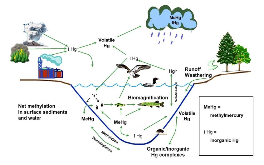
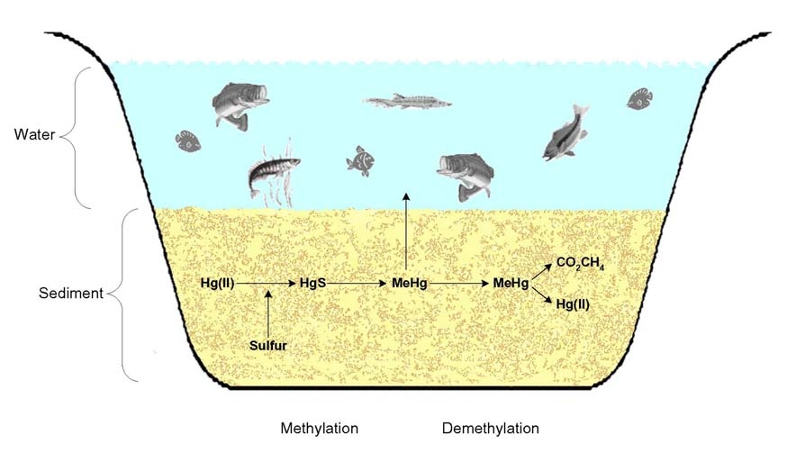
- Figure 2 Mercury Methylation
- Figure 1
- The Mercury Cycle
- Experience:
- PROJECT RELATED EXPERIENCE – ECOTOXICOLOGY/TOXICITY TESTING
- Example Publications International Peer-Reviewed Literature
- PROJECT RELATED EXPERIENCE – ENVIRONMENTAL RISK ASSESSMENT
- Example Publications International Peer-Reviewed Literature
- Example Publications International Peer-Reviewed Literature
- PROJECT RELATED EXPERIENCE – EXPERT WITNESS AND PEER REVIEW
- Peer Reviewer USA, Canada, Australasia, Europe
- PROJECT RELATED EXPERIENCE – METALS AND METALLOIDS
- Example Publications International Peer-Reviewed Literature
- PROJECT RELATED EXPERIENCE – SEWAGE EFFLUENT AND TREATMENT
- Example Publications International Peer-Reviewed Literature
- JOURNAL PUBLICATIONS [* = Editorials or Letters to the Editor]
- CHAPTERS IN BOOKS
- LEARNED DISCOURSES
- Peter M. Chapman
- INTRODUCTIONS TO DEBATES/COMMENTARIES
- Peter M. Chapman
- EDITORIAL PUBLICATIONS
- Peter M. Chapman
- PUBLISHED PROCEEDINGS
- Peter M. Chapman
- Peter M. Chapman
- Peter M. Chapman
- Peter M. Chapman
- Peter M. Chapman
- PUBLISHED TECHNICAL REPORTS AND THESES
- Peter M. Chapman
- Peter M. Chapman
- CO-AUTHORED U.S. EPA SCIENCE ADVISORY BOARD (SAB) REPORTS
- Peter M. Chapman
- PUBLISHED ABSTRACTS
- Peter M. Chapman
- Peter M. Chapman
- Peter M. Chapman
- Peter M. Chapman
- Peter M. Chapman
- Peter M. Chapman
- Peter M. Chapman
- Peter M. Chapman
- Peter M. Chapman
- UNPUBLISHED MANUSCRIPTS AND REPORTS
- Peter M. Chapman
- Peter M. Chapman
- Peter M. Chapman
- Peter M. Chapman
- Peter M. Chapman
- Peter M. Chapman
- Peter M. Chapman
- Peter M. Chapman
- Peter M. Chapman
- Peter M. Chapman
- Exhibit 1
- Mercury
- Blood mercury concentration (μg per liter)
- 5% poorerperformancein Faroes
- Lower limit
- on 85
- 0.8 5.8
- EPA reference
- (women ofchildbearing
- 0 100
- 0.8 5.8
- Exhibit 4
- Blood mercurylevel comparison5.7% US
- women
- Hair mercury level (ppm)
- 5%increasein
- abnormalBoston
- NamingTest
- responses
- Faroe Islands
- Average
- EPAreference
- ge
- percentile
- Exhibit 5Hair mercury level
- comparison
- Japanese
- average
- ATSDR EPA RIVM WHO ICF/TERA
- Exposure
- Uncertainty
- Change assumption as per
- Relative source
- Resulting fish tissue
- concentration limit(mg/kg or ppm)
- BEFORE THE ILLINOIS POLLUTION CONTROL BOARD
- IN THE MATTER OF:
- PROPOSED NEW 35 ILL.ADM.CODE PART 225 CONTROL OF EMISSIONS FROM
- LARGE COMBUSTION SOURCES
- ) ) ) )
- PCB R06-25 Rulemaking - Air
- EXECUTIVE SUMMARY
- A REVIEW OF
- THE STATUS OF MERCURY CONTROL TECHNOLOGY
- SECTION 1
- INTRODUCTION
- SECTION 2
- ILLINOIS PROPOSED RULE: WHAT DOES IT REALLY ASK?
- SECTION 3
- EVOLUTION AND COST OF ENVIRONMENTAL CONTROL TECHNOLOGY
- SECTION 4
- INHERENT MERCURY REMOVAL FROM ENVIRONMENTAL CONTROLS
- SECTION 5
- MERCURY SPECIFIC CONTROL TECHNOLOGIES
- (MW)
- FGD Type/SO2 Inlet
- Baseline Hg Removal vs. with Additive
- Hg Removal
- Test
- Duration
- Date
- Design Coal
- PresentCoal
- Initial/Final ESP SCA
- 2/kacfm)
- Description of ESP Upgrade
- ESP SCA, ft2/kacfm
- Hg removal, %
- (tons/year)
- ACI-Induced PM
- Emissions
- (tons/year at 98.3%
- efficiency)
- ACI-Induced PM
- Emissions
- (tons/year at 95% efficiency)
- SECTION 6
- PROCESS GUARANTEES
- SECTION 7
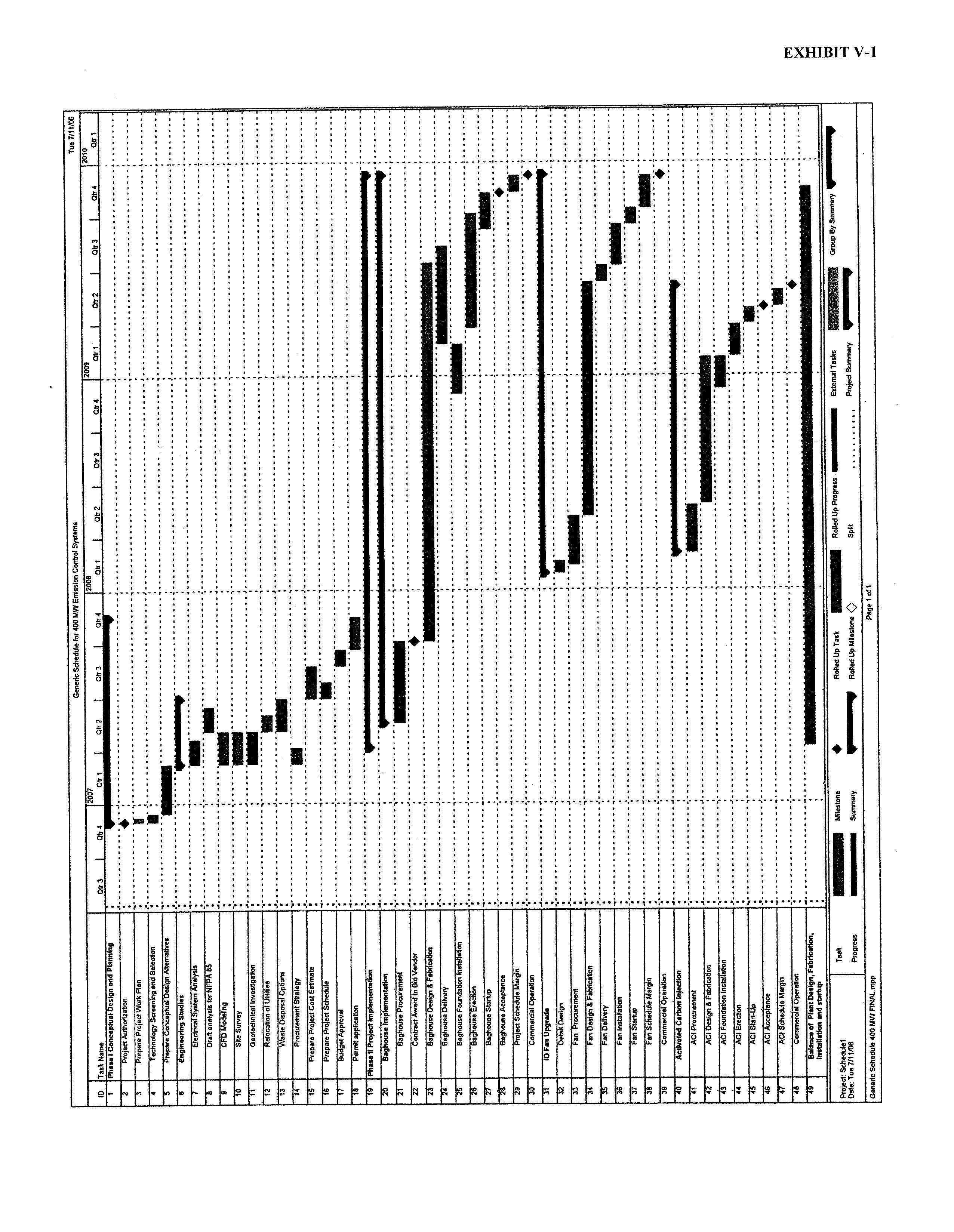
- SCHEDULE AND DEMONSTRATION PLANS
- SECTION 8
- CONCLUSIONS
- REFERENCES
- APPENDIX A
- SUMMARY OF ASSUMPTIONS DEFINING
- SECTION A-1
- INTRODUCTION
- SECTION A-2
- INHERENT REMOVAL AND BASELINE HG EMISSIONS
- Table A.2-1. EMF Recommendations
- Control Configuration Bituminous
- Coal
- Sub-bituminous Lignite
- Table A.2-2. Summary of Factors in the FBC Correlation
- SECTION A-3
- ACTIVATED CARBON INJECTION (ACI) IN PM CONTROLS
- SECTION A-4
- ACI/FABRIC FILTER
- SECTION A-5
- CARBON INJECTION: SPRAY DRYER ABSORBER (SDA)/FF
- Note 1 all ESP HACI 90% 6.5
- SECTION A-6
- SCR AND FGD HG REMOVAL
- SECTION A-7
- FLUID BED UNITS: ACI/FABRIC FILTER (COHPAC/TOXECON)
- APPENDIX A REFERENCES
- APPENDIX B
- ASSUMPTIONS DEFINING THE PERFORMANCE AND COST
- OF SO2, NOx, AND PARTICULATE MATTER FOR
- CAIR COMPLIANCE
- SECTION B-1
- INTRODUCTION
- SECTION B-2
- FLUE GAS DESULFURIZATION CONTROL TECHNOLOGY
- Table B-1 - Wet FGD Design and Operating Variables
- Figure B-1 – Conventional Wet FGD Capital Cost Estimates
- Figure B-2 – Fixed O&M Costs: Conventional Wet and Dry FGD
- Figure B-3. Dry FGD Capital Cost
- Figure B-4. Dry FGD Fixed Operating Costs
- SECTION B-3
- NITROGEN OXIDES (NOx) CONTROL TECHNOLOGY
- Table B-3. SCR Fixed, Variable Operating Costs
- Coal Source Minimum NOx Outlet Rate
- (lbs/MBtu)
- SECTION B-4
- PARTICULATE MATTER CONTROL TECHNOLOGY
- SECTION B-5
- ACTIVATED CARBON INJECTION HARDWARE
- SECTION B-6
- ACI/FABRIC FILTER (COHPAC/TOXECON) for FLUIDIZIED BED UNITS
- APPENDIX B REFERENCES
- BEFORE THE ILLINOIS POLLUTION CONTROL BOARD
- IN THE MATTER OF:
- PROPOSED NEW 35 ILL.ADM.CODE PART 225 CONTROL OF EMISSIONS FROM
- LARGE COMBUSTION SOURCES
- ) ) ) )
- PCB R06-25
- TESTIMONY OF MR. WILLIAM DEPRIEST
- I. INTRODUCTION
- II. DESIGN DECISION IMPACTS OF THE PROPOSED ILLINOIS
- 1. CAIR and CAMR emission reduction timelines were drafted to allow
- 2. If the phased mercury control approach of CAMR is eliminated, most
- III. RETROFIT DIFFICULTIES THAT AFFECT THE COSTS OF MERCURY
- CONTROL ON THE ILLINOIS COAL-FIRED POWER PLANTS
- 1. Capabilities of the Existing Electrostatic Precipitator (ESP) to
- 2. Fan Upgrades Required Due to Existing Fan Limitations
- 3. Electrical Distribution Upgrades Due to Existing Infrastructure
- Limitations
- 4. Infrastructure Limitations
- 5. Physical Limitations of Existing ESPs, Existing Ductwork
- Configurations, and Existing Plant Layouts
- 6. Outage Limitations
- 7. Waste Disposal Limitations
- IV. CURRENT MARKET FACTORS THAT AFFECT THE COST AND
- SCHEDULE OF COMPLIANCE WITH THE PROPOSED ILLINOIS MERCURY RULE
- 1. Design and Manufacturing Capabilities
- 2. Labor Market
- 3. Seller’s Market
- 4. Steel and Alloy Market Volatility
- 5. Outage Costs and Impacts
- 6. Owner Resources and Contracting Approaches
- V. EXPECTED PROJECT IMPLEMENTATION SCHEDULES FOR
- MEASURES REQUIRED TO COMPLY WITH THE PROPOSED ILLINOIS MERCURY RULE
- VI. INSTALLED COST PROJECTIONS FOR RETROFITS EXPECTED TO
- MERCURY RULE
- 1. Cost Ranges for Sorbent Injection Alone
- 2. Cost Ranges for Polishing Fabric Filter Plus Sorbent Injection
- Unit Size
- Retrofit Complexity Moderate
- Retrofit Complexity
- Difficult
- Retrofit Complexity
- Severe
- 3. Cost Ranges For Full Pulse Jet Fabric Filter to be Used in
- Conjunction with Dry FGD and Sorbent Injection
- Two Stage Compliance ($/kw)
- Phase 1: Activated Carbon and Pulse Jet Fabric Filter
- Phase 2: Addition for Dry FGD
- Unit Size
- Retrofit Complexity
- Moderate
- Retrofit Complexity
- Difficult
- Retrofit Complexity
- Severe
- BEFORE THE ILLINOIS POLLUTION CONTROL BOARD
- IN THE MATTER OF:
- PROPOSED NEW 35 ILL.ADM.CODE PART 225 CONTROL OF EMISSIONS FROM
- LARGE COMBUSTION SOURCES
- ) ) ) )
- PCB R06-25 Rulemaking - Air
- I. QUALIFICATIONS
- II. INTRODUCTION
- III. IL MERCURY RULE
- IV. METHODOLOGY AND CONTROL ASSUMPTIONS
- V. COMPARISON OF COMPLIANCE EFFECTS OF MEETING
- CAIR/CAMR AND CAIR/IL MERCURY RULE FOR IL GENERATORS
- TABLE 1
- IL COAL- & GAS/OIL-FIRED GENERATION: 2005 - 2018
- (GWh)
- TABLE 2
- SO2, NOx and MERCURY EMISSIONS FROM IL GENERATORS
- (SO2 & NOx in tons and Hg in pounds)
- TABLE 3
- CAPITAL INVESTMENT OF SO2, NOx AND MERCURY CONTROL
- TECHNOLOGIES: 2009 – 2018
- (billions of 2006 $)
- TABLE 4
- COMPARISON OF CUMULATIVE ANNUALIZED COMPLIANCE COSTS FOR
- SO2, NOx AND MERCURY CONTROLS: 2009-2018
- (billions of 2006 $)
- VI. SUMMARY OF COMPLIANCE ISSUES
- VII. COMPARISON OF COMPLIANCE COSTS
- TABLE 5
- COMPARISON FOR MERCURY CONTROL COMPLIANCE COSTS
- (in 2006 million dollars)
- MCH TSD ICF
- Capital Investment
- TABLE 6
- MCH AND TSD COMPARATIVE UNIT TECHNOLOGY COSTS: $/kW
- (in 2006 dollars)
- APPENDIX A
- METHODOLOGY AND INPUT ASSUMPTIONS
- TABLE A-1
- NOx UNIT ALLOCATION SCHEDULE UNDER CAIR
- TABLE A-2
- MERCURY UNIT ALLOCATION SCHEDULE UNDER CAMR
- TABLE A-3
- CAIR AND CAMR ALLOWANCE PRICES
- (2006 $)
- I. BACKGROUND AND QUALIFICATIONS
- II. ANALYSIS OF ELECTRICITY MARKET
- OPERATIONS
- Coal Description Heating Value
- (Btu/lb)
- SO2 Content (lbs/MMBtu)
- Hg Content (lbs/TBtu)
- Coal Type 2006 2008 2009 2010 2013 2015 2018
- Allowance Type 2006 2008 2009 2010 2013 2015 2018
- BEFORE THE ILLINOIS POLLUTION CONTROL BOARD
- TESTIMONY OF RICHARD D. McRANIE
- Executive Summary
- Qualifications
- Introduction
- Brief Description of the Proposed Illinois Rule
- Overview Discussion of Hg Measurements Required
- General Discussion of the Probable Monitoring Issues
- Significant Figures
- Historical Perspective of Hg Emissions Monitoring
- Hg Monitoring Technology
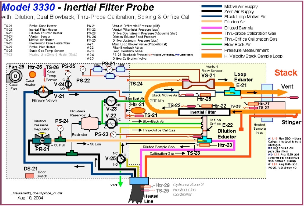
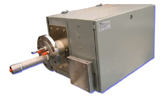
- Figure 1 – Tekran Hg CEMS Inertial Filter Probe
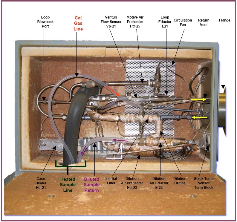
- Figure 2 – Tekran Probe Box
- Figure 3 – Tekran Probe Box - Hot-side
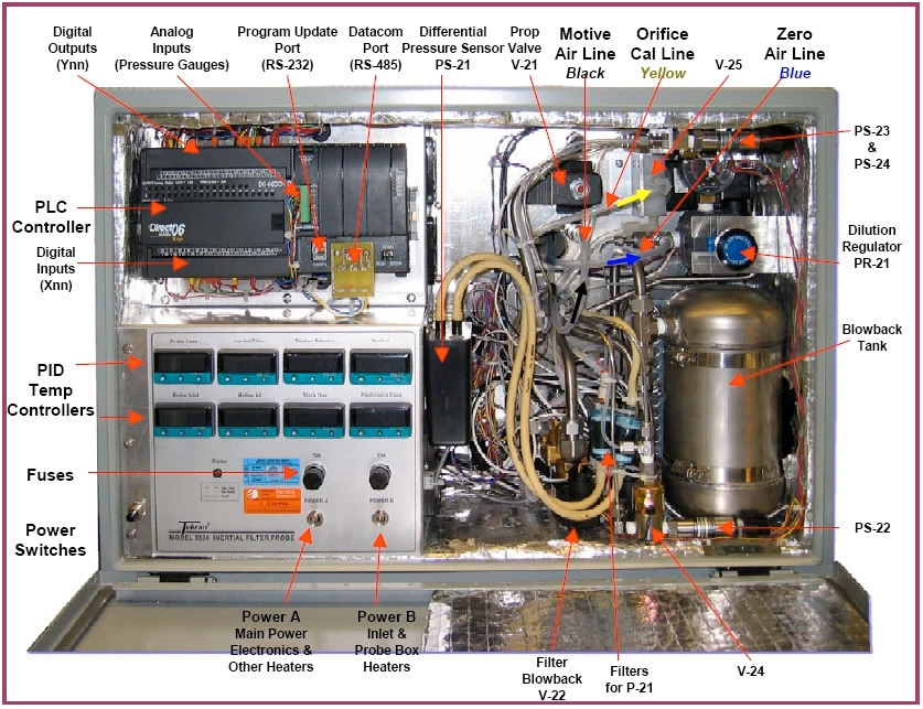
- Figure 4 – Tekran Probe Box – Cold Side
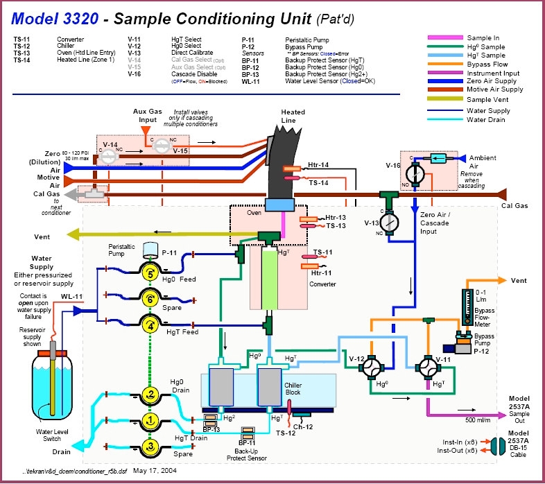
- Figure 5 – Tekran Sample Conditioning Unit
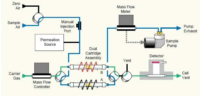
- Figure 6 – Tekran Hg Analyzer Flow Diagram
- Calibration Issues with Hg CEMS
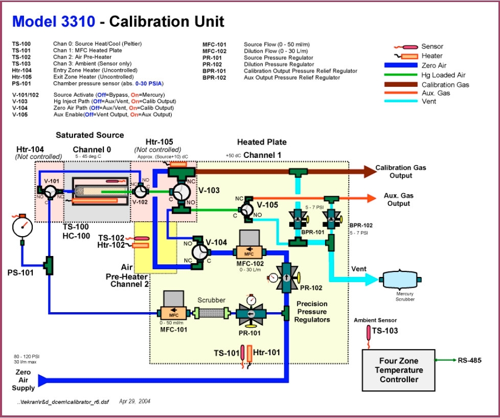
- Figure 7 – Tekran Elemental Hg Calibrator Flow Diagram
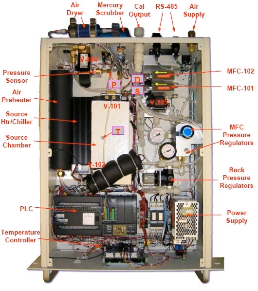
- Figure 8 – Tekran Calibrator Internal View
- Figure 9 – Oxidized Hg Calibrator Flow Diagram
- Figure 10 – HovaQuick Oxidized Hg Calibrator
- Measurement Characteristics
- Figure 11 – Example Normal Distribution
- Figure 12 – Example Log Normal Distribution
- Figure 13 - High accuracy but low precision
- Figure 14 - High precision but low accuracy
- Description of Hg Monitoring and Demonstration Research Projects
- Table 1 - RATA 1 Results From Trimble County
- RATA Criteria Tekran Thermo Horiba Forney
- Table 2 - RATA 2 Results From Trimble County
- RATA Criteria Tekran Thermo Opsis Durag
- EPRI Hg Monitoring Demonstration Project and Results
- Figure 13 – Inertial Probe Loop Exit Plugging
- Table 3. Calibration Error Test Results - CEMS X - April 2006
- Zero Error Span Response Error
- Date Response (% of Span) (Expected 9.8ug/m
- 3 ) (% of Span)
- Table 4. Calibration Error Test Results - CEMS X - May 2006
- Table 5. Calibration Error Test Results – CEMS Y - May 2006
- Missing Data Substitution
- Coal Sampling and Analysis Error Sources
- Propagation of Error
- Hg Data Discussion
- Figure 14 – Hg CEMS Readings – Trimble County
- Figure 15 – Hg CEMS Readings – Trimble County
- Figure 16 – Hg CEMS Readings – Trimble County
- Figure 17 – Hg CEMS Readings – Trimble County
- SCR damper opened
- NH3 injection began
- Conclusions
- Appendix 1
- Appendix 2
- Conversion Protocollb/GWh Hg to microgram/m
- Equation 1
- 10 Btu
- 0.80 10 lb Hg
- 10 Btu
- 0.80 lb Hg
- 10,000Btu
- 1 kW hr
- 1 10 kW
- GW hr
- 0.008 lbHg
- Equation 2
- EC F
- Equation 3
- 100
- 1,800
- 0.80 10C
- BEFORE THE ILLINOIS POLLUTION CONTROL BOARD
- IN THE MATTER OF:
- PROPOSED NEW 35 ILL.ADM.CODE PART 225 CONTROL OF EMISSIONS FROM
- LARGE COMBUSTION SOURCES
- ) ) ) )
- PCB R06-25
- which is detrimental to its use in concrete.
- concrete.
- concrete.
- fly ash has been in contact with an activated carbon sorbent.
- Education:
- Current Employment
- February 2003 – present, University of Illinois at Chicago
- April 1998 – Present, Ish Inc.
- Previous Employment
- Business Experience
- Technical and Professional Experience
- National Committees Experience
- Publication and Presentations
- Current Service on University Committees
- Recently completed and ongoing projects on Coal Ash Management
- BEFORE THE ILLINOIS POLLUTION CONTROL BOARD
- IN THE MATTER OF:
- PROPOSED NEW 35 ILL.ADM.CODE PART 225 CONTROL OF EMISSIONS FROM
- LARGE COMBUSTION SOURCES
- ) ) ) )
- PCB R06-25 Rulemaking - Air
- TESTIMONY OF KRISH VIJAYARAGHAVAN
- I. INTRODUCTION
- A. AER credentials
- B. Witness credentials
- II. ATMOSPHERIC MERCURY
- III. CHEMICAL TRANSPORT MODELS
- IV. THE TRACE ELEMENT ANALYSIS MODEL (TEAM)
- VI. COMPARISON OF TEAM SIMULATION RESULTS WITH OTHER
- INFORMATION IN THE ILLINOIS PCB RECORD
- Mercury wet deposition in Steubenville, Ohio
- VII. OTHER COMMENTS ON INFORMATION IN THE ILLINOIS PCB
- RECORD
- Receptor-based models
- Meteorological analysis of Dr. Keeler
- Massachusetts analysis
- Florida analysis
- REFERENCES
- Attachment A
- KRISH VIJAYARAGHAVAN
- Atmospheric and Environmental Research, Inc. August 1997 - present
- Aspen Technology, Inc., Cambridge, MA
- I. BACKGROUND AND QUALIFICATIONS
- II. ANALYSIS OF ELECTRICITY MARKET OPERATIONS
- Coal Description Heating Value
- (Btu/lb)
- SO2 Content (lbs/MMBtu)
- Hg Content (lbs/TBtu)
- Coal Type 2006 2008 2009 2010 2013 2015 2018
- Allowance Type 2006 2008 2009 2010 2013 2015 2018
- CERTIFICATE OF SERVICE
- SERVICE LIST
- (R06-25)
- SERVICE LIST
- (R06-25)
|
BEFORE THE ILLINOIS POLLUTION CONTROL BOARD
IN THE MATTER OF:
PROPOSED NEW 35 ILL.ADM.CODE PART 225
CONTROL OF EMISSIONS FROM
LARGE COMBUSTION SOURCES
)
)
)
)
)
PCB R06-25
Rulemaking - Air
NOTICE OF FILING
To:
Dorothy Gunn, Clerk
Illinois Pollution Control Board
James R. Thompson Center
Suite 11-500
100 West Randolph
Chicago, Illinois 60601
Persons included on the
ATTACHED SERVICE LIST
PLEASE TAKE NOTICE that we have today filed with the Office of the Clerk of the
Pollution Control Board the
Testimony
of the following witnesses, copies of which are herewith
served upon you:
Peter M. Chapman, Ph.D.; Gail Charnley, Ph.D., and Attached Exhibits;
J.E. Cichanowicz; William DePriest and Attached Exhibits; James Marchetti; Richard D.
McRanie; Ishwar Prasad Murarka, Ph.D.;
and
Krish Vijayaraghavan
.
/s/
Kathleen C. Bassi
Kathleen C. Bassi
Dated: July 28, 2006
Sheldon A. Zabel
Kathleen C. Bassi
Stephen J. Bonebrake
Joshua R. More
Glenna Gilbert
SCHIFF HARDIN, LLP
6600 Sears Tower
233 South Wacker Drive
Chicago, Illinois 60606
312-258-5500
ELECTRONIC FILING, RECEIVED, CLERK'S OFFICE JULY 28, 2006
Page 1
BEFORE THE ILLINOIS POLLUTION CONTROL BOARD
IN THE MATTER OF:
PROPOSED NEW 35 ILL.ADM.CODE PART 225
CONTROL OF EMISSIONS FROM
LARGE COMBUSTION SOURCES
)
)
)
)
)
PCB R06-25
TESTIMONY OF PETER M. CHAPMAN, Ph.D.
Back to top
1.0 Qualifications
My name is Peter M. Chapman. I am an internationally recognized expert in the fields of
aquatic ecology, ecotoxicology, and environmental risk assessment, with particular
expertise and experience in the environmental fate and effects of metals including
mercury. I have published over 150 scientific journal articles and book chapters, written
over 200 technical reports, and made over 100 presentations at scientific meetings. I am
Senior Editor of the international peer-reviewed journal,
Human and Ecological Risk
Assessment
, a member of the Editorial Boards of two other international journals, editor
of a popular, on-going series of scientific discourses, and have held advisory
appointments with the National Research Councils of both Canada and the United States
as well as with the USEPA Science Advisory Board. In 2001 the Society of
Environmental Toxicology and Chemistry (SETAC) awarded me its Founders Award,
their most prestigious award for an outstanding career and contributions to the
environmental sciences. Since 1999 I have been part of the Natural Sciences and
Research Council (NSERC)-funded network of university researchers originally titled
“Metals in the Environment” [www.mite-rn.org] and now titled “Metals in the Holistic
Environment” [www.mithe-rn.org]. My role in the Network is to integrate the work done
by researchers and universities participating in the Network into a risk assessment
framework for decision-making. My specific focus in this regard is metals including
mercury in aquatic ecosystems. My curriculum vita is provided as Attachment 1.
Page 2
2.0 Summary of Testimony
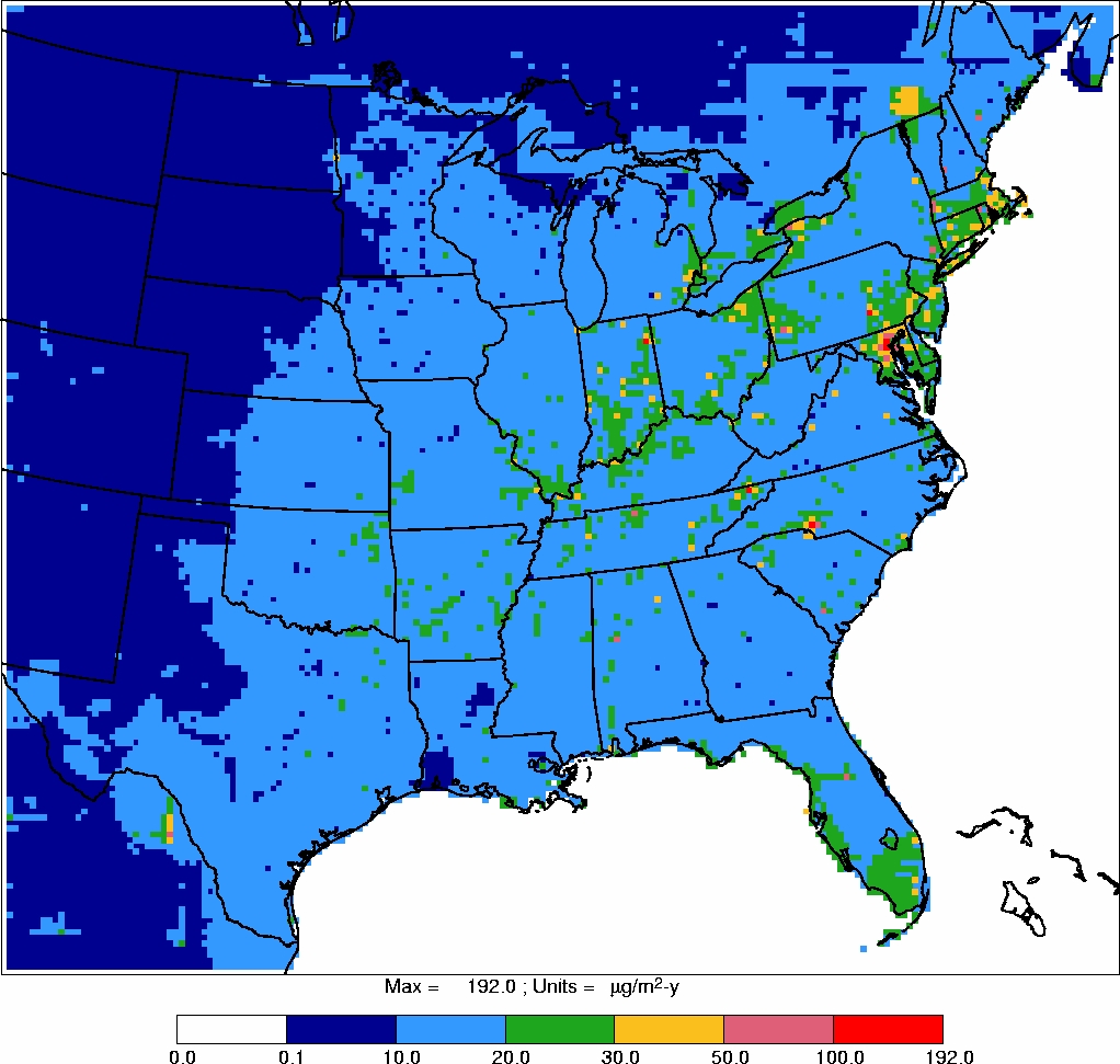
My testimony initially explains what happens to mercury when it is deposited from the
atmosphere or other sources into aquatic environments. I then evaluate the possibility of a
linkage between mercury emissions from coal-fired power plants in Illinois and mercury
in fish in Illinois waters related to lifting impaired water restrictions.
The basis for Illinois EPA’s proposed mercury rule is well summarized in the testimony
of Jim Ross at page 5: "A key concept in understanding the need and methods for
mercury control is that although mercury air emissions are the target for reductions, the
ultimate goal is to reduce methyl mercury levels in water bodies and, hence, fish tissue."
Accordingly, the focus of my testimony is this “key concept”; specifically, my testimony
answers the following two key questions:
Question 1:
Will reducing inorganic mercury emissions from coal-fired power plants in
Illinois under the proposed rule reduce organic (methyl) mercury concentrations in fish
living in water bodies in Illinois to the same extent?
Question 2:
Will reducing inorganic mercury emissions from coal-fired power plants in
Illinois under the proposed rule ensure that impairment restrictions can be lifted for
water bodies where fish have elevated mercury concentrations?
The answer to both of these questions, as my testimony clearly demonstrates, is “No”.
The goal of the proposed rule, as summarized in Marcia Willhite’s written testimony at
page 4 (“In order to assure that 95% of largemouth bass in Illinois waters may be
consumed in unlimited quantities by sensitive subpopulations, a 90% reduction of
mercury in fish tissue is needed”), will not be achieved.
Page 3
3.0 Mercury in the Environment
The relationship between inorganic mercury emissions and organic mercury in the
environment including fish is complex
1
.
For instance, when mercury is emitted from
coal-fired power plants it is as an inorganic substance – typically elemental mercury
(Hg
0
), divalent mercury (Hg
2+
, also termed reactive gaseous mercury, or RGM), and
particulate mercury
2
, and can change form as it travels downwind
3
. Inorganic mercury is
also emitted from a wide variety of other sources including motor vehicles, incinerators,
crematoria, forest fires, deep sea vents, volcanoes, oceans, soils, etc
4
. Although estimates
vary, about half the mercury emitted to the atmosphere is natural, and about half is due to
human activities
5
. All states and countries have some level of mercury emissions; the
greatest current levels of human emissions appear to be from China related to its rapid
industrialization
6
.
Contamination due to mercury is a world-wide problem
7
.
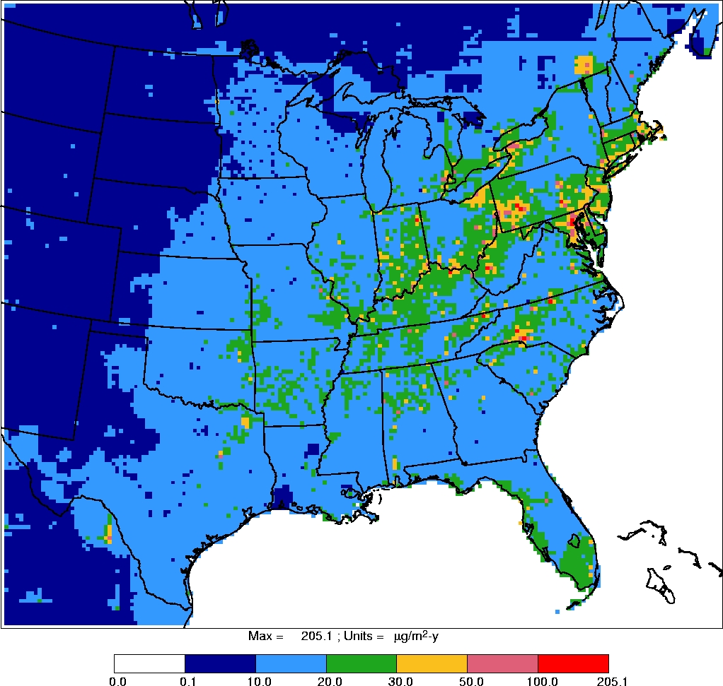
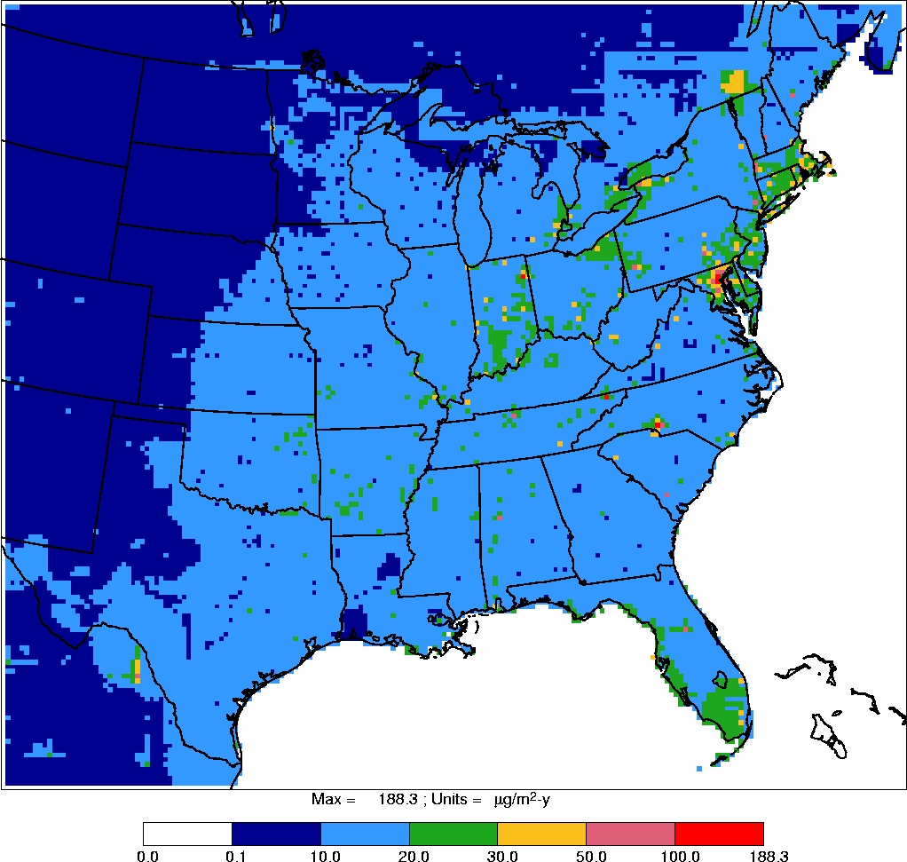
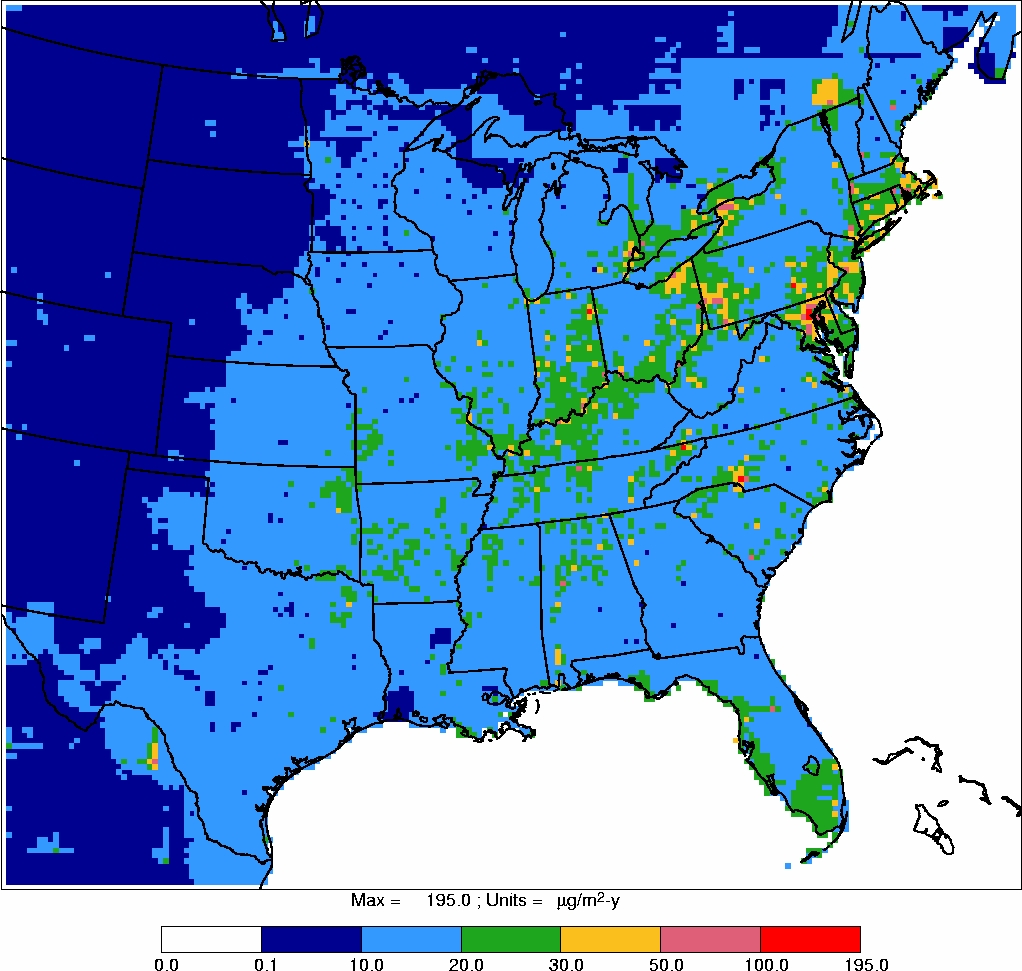
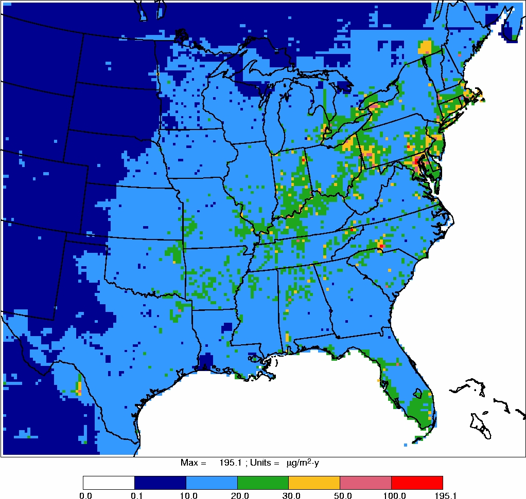
Mercury in the atmosphere can be deposited onto land or water via either dry deposition
(e.g., dust) or wet deposition (e.g., rain, snow)
8
. Wet deposition can result in some forms
of mercury coming down closer to emission sources than others. But mercury deposited
to land or water may not remain there; mercury can be re-emitted back to the atmosphere
where it is transported further. For instance, Dr. Keeler (one of Illinois EPA’s witnesses)
and his co-workers have shown that re-emission of dissolved gaseous mercury from Lake
1
Eisler R. 2006. Mercury Hazards to Living Organisms. Published by Taylor and Francis, Boca Raton, FL,
USA.
2
Marcia Willhite’s verbal testimony on June 14, 2006: at page 32 of the transcript of that testimony.
3
Lohman K, Seigneur C, Edgerton E, Jansen J. 2006. Modeling mercury in power plant plumes. Environ
Sci Technol 40: 3848-54.
4
Eisler 2006, op. cit.; also, written testimony of Gerald Keeler at page 3, indicates that motor vehicle
sources contribute mercury to the atmosphere.
5
USEPA. 2005. Mercury emissions: The global context.
www.epa.gov/mercury/control_emissions/global.htm
; also, Landis MS, Vette AF, Keeler GJ. 2002.
Atmospheric mercury in the Lake Michigan basin: Influence of the Chicago/Gary urban area. Environ Sci
Technol 36: 4508-17.
6
Seigneur C, Vijayarghavan K, Lohman K, Karamchandani P, Scott C. 2004. Global source attribution for
mercury deposited in the United States. Environ Sci Technol 38: 555-69; also, Jiang G-B, Shi J-B, Feng X-
B. 2006. Mercury pollution in China. Environ Sci Technol 40: 3673-8; also, Gerald Keeler’s verbal
testimony on June 15, 2006: at page 17 of the transcript of that testimony.
7
Eisler 2006, op. cit.; also, Gerald Keeler’s verbal testimony on June 15, 2006: at page 17 of the transcript
of that testimony.
8
Dvonch JT, Graney JR, Keeler GJ, Stevens RK. 1999. Use of elemental tracers to source apportion
mercury in south Florida precipitation. Environ Sci Technol 33: 4522-7.
Page 4
Michigan is a process that significantly reduces net atmospheric deposition
9
. In fact, Dr.
Keeler in testimony before the U.S. House of Representatives stated, “…previously
deposited mercury can also undergo chemical transformations that convert it back to the
elemental form that readily leaves the earth’s surface (land and water) to re-enter the
global background of mercury”
10
. Similarly, Illinois EPA’s Technical Support Document
(the “TSD”) mentions mercury volatilizing from water back into the atmosphere. Thus,
once mercury enters the atmosphere, it becomes part of a global cycle of mercury
among land, water, and the atmosphere; past activities continue to affect current
atmospheric mercury concentrations
11
.
The inorganic mercury that remains in water bodies (either from the atmosphere or from
other sources) can undergo different biological and physico-chemical processes (Figure
1). The mercury cycle is a complex biogeochemical system involving both biotic and
abiotic transformations of the different forms of mercury. Inorganic mercury species that
are not reduced to form gaseous elemental mercury have an affinity for particulates and
organic matter and thus will tend, if not re-emitted, to sink down to and accumulate in the
sediments. The sediments of water bodies thus serve as both a sink and a reservoir for
mercury contamination. They can also be a source of potential mercury pollution
12
.
Although most inorganic mercury remains in this form in the sediments, a portion
13
of
that mercury can be converted to an organic form of mercury, methyl mercury. This
conversion occurs primarily by metabolism within sulphate- and iron-reducing bacteria
living in anaerobic sediments, i.e., sediments without oxygen
14
. Mercury methylation
9
Landis MS, Keeler GJ. 2002. Atmospheric mercury deposition to Lake Michigan during the Lake
Michigan mass balance study. Environ Sci Technol 36: 4518-24; Vette AF, Landis MS, Keeler GJ. 2002.
Deposition and emission of gaseous mercury to and from Lake Michigan during the Lake Michigan mass
balance study (July, 1994 – October, 1995). Environ Sci Technol 36: 4525-32.
10
Keeler GJ. 2001. The problem of mercury. Testimony for the U.S. House of Representatives Committee
on Science Hearing on Acid Rain: The State of the Science and Research Needs for the Future. May 3,
2001.
11
Eisler 2006, op. cit.
12
Eisler 2006, op. cit.
13
Marcia Willhite’s verbal testimony on June 14, 2006 states “it has been estimated that .7 to .0006 percent
of total mercury in sediment is methylmercury”: at page 40 of the transcript of that testimony.
14
Fleming EJ, Mack EE, Green PG, Nelson DC. 2006. Mercury methylation from unexpected sources:
Molybdate-inhibited freshwater sediments and an iron-reducing bacterium. Appl Environ Microbiol 72:
457-64; also, Jeremiason JD, Engstrom DR, Swain EB, Nater EA, Johnson BM, Almendinger JE, Monson
Page 5
generally cannot occur in aerobic (oxygenated) environments; in the water column it can
occur only when conditions are anoxic (there is no oxygen). Methyl mercury production
occurs not just in recently deposited surface sediments but also in much older, deeper
sediments where the mercury was deposited decades previously, even though “old”
inorganic mercury in sediments tends to be less biologically available than “new”
inorganic mercury in sediments
15
. Methyl mercury from these deeper sediments can reach
organisms living in shallower sediments by a process called diagenesis, which typically
occurs in sediments with low organic carbon content. There is a depth beyond which,
absent unusual disturbances, the mercury in the sediments will not reach animals or
plants, but burial to such a depth is typically a slow process under natural conditions. As
noted in the Florida study there is “slow mobilization of historically deposited mercury
from deeper sediment layers to the water column. Until buried below the active zone, this
mercury can continue to cycle through the system”
16
. Thus, even when emissions of
inorganic mercury are reduced, there will be a substantial lag phase before emission
reductions can result in reductions in methyl mercury concentrations in fish.
Production of methyl mercury in sediments is not a readily predictable process and can
be highly variable between water bodies
17
(Table 1). There is not a 1:1 relationship
between inorganic mercury released to the atmosphere and deposited in water bodies and
the level of methyl mercury found in water bodies and fish tissue. For instance, methyl
mercury produced in water bodies from inorganic mercury deposition can be augmented
by direct precipitation of methyl mercury from other sources, including: the atmosphere,
runoff from land, or inputs from other water bodies such as wetlands
18
.
BA, Kolka RK. 2006. Sulfate addition increases methylmercury production in an experimental wetland.
Environ Sci Technol 40: 3800-6.
15
Fleming et al. 2006, op. cit.
16
Florida Dept of Environmental Protection. 2003. Integrating atmospheric mercury deposition with
aquatic cycling in South Florida: An approach for conducting a total maximum daily load analysis for an
atmospherically derived pollutant: at page iii.
17
Marcia Willhite’s verbal testimony on June 14, 2006 notes that the characteristics that impact mercury
methylation are water body specific, can differ between water bodies, and that mercury methylation is
highly dependent on water chemistry and biology, in particular pH, dissolved oxygen, dissolved organic
carbon, nutrients, selenium concentrations, temperature, sulphate concentrations, drainage size to lake
volume ratio, percentage of wetland and watershed, conductivity and water level flucturations: at pages 45
to 47 of the transcript of that testimony. She made similar comments elsewhere in her verbal testimony:
e.g., at page 37 of the transcript of that testimony.
18
Eisler 2006, op. cit.
Page 6
Table 1
Example of Physico-Chemical Processes Affecting Mercury Methylation
19
Physico-Chemical Condition
Methylation
Enhanced
↑
Decreased
↓
Low dissolved oxygen
Yes
Low pH
Yes
(in water)
Yes
(in sediment)
Increased dissolved organic carbon
Yes
(in sediment)
Yes
(in water)
Increased conductivity or salinity
Yes
Increased nutrients
Yes
Increased selenium
Yes
Increased temperature
Yes
Increased sulphate or sulphide
Yes
Point and non-point source discharges continue to contribute mercury to water bodies.
For example, Marcia Willhite notes at page 144 of the transcript of her June 14, 2006
verbal testimony, that runoff may be a significant source of mercury in southern Illinois.
Interestingly, at page 118 of the transcript of that same testimony, Ms Willhite notes that
historical data suggest that the levels of mercury in fish are higher than expected in
waters in the far southern end of the State.
The TSD indicates (at pages 68 and 69, including Table 4.7) that, at “maximum”
discharge levels, the 137 wastewater point sources in Illinois would discharge
approximately 1.5 tons of mercury per year compared to 45 pounds at an “average”
discharge level. Marcia Willhite confirmed in her testimony (June 14, 2006, at pages 288-
290 of the transcript) that the “maximum” load or discharge level was based on actual
measured maximum flow and maximum mercury concentrations in the flow, which
would comprise approximately 1.5 tons, or about half of the mercury air emissions from
coal-fired power plants as indicated in the TSD (3 tons at page 60). Other un-measured
sources of mercury exist including combined sewer overflows, which Illinois EPA does
not sample for mercury but which contain mercury
20
. Thus other local sources of mercury
19
Developed based on information contained in Eisler 2006, op. cit.
20
Available data on mercury related to combined sewer overflow discharges for the Metropolitan Water
Reclamation District of Greater Chicago reviewed by Dr. Chapman suggest that inputs can be on the order
of tens of pounds per year.
Page 7
(as well as sources outside the State) will have inputs to different water bodies that likely
are, in some cases, greater than those from coal-fired power plants.
Similarly, production of methyl mercury in the sediments of water bodies is governed by:
microbial community composition, geochemical conditions that affect the activity of
methylating bacteria (e.g., availability of carbon, abundance of electron acceptors such as
sulphate), and availability of inorganic mercury in a suitable (bioavailable) form for
methylation. Availability of carbon and the cycling of sulphur are major constraints on
the process of mercury methylation. For instance, although sulphate is essential for the
methylation process, excessive amounts of sulphate can actually poison the mercury
methylation process by limiting the availability of mercury to methylating bacteria. The
key Florida study cited in the TSD notes, “Sulfate is an important influence on the
production of methylmercury, affecting not only mercury transformations, but also the
biological availability of mercury for uptake….[sulphate] is an important cofactor
controlling the severity of the mercury problem at any given site”
21
. Methyl mercury
concentrations in fresh water bodies in the U.S. may have increased historically due to
increases in atmospheric sulphate deposition.
Decreases in sulphate deposition alone,
with no change in mercury inputs, could result in lower methyl mercury levels in
freshwater fish
22
. It is thus entirely possible that reductions in sulphate deposition rates
resulting from the Acid Deposition Program were at least partly responsible for decreased
methyl mercury concentrations seen, for instance, in Massachusetts from 1999 to 2004.
In addition, demethylation can occur in sediments (Figure 2), also mediated by naturally
occurring microbes – possibly as a defense against mercury toxicity
23
. In most, but not all
anaerobic systems, mercury methylation rates are greater than demethylation rates.
However,
methyl mercury concentrations and production rates vary more than do
inorganic mercury deposition rates
. For instance, a simple change in bacterial activity
alone could “cause an increase in fish mercury concentrations even as atmospheric
21
Florida Dept of Environmental Protection 2003, op. cit., at page vi.
22
Jeremiason et al. 2006, op. cit.
23
Eisler 2006, op. cit.
Page 8
deposition [from industrial mercury emissions] decreases”
24
. Thus there can be, for
instance, freshwater systems containing relatively high concentrations of inorganic
mercury but relatively low concentrations of methyl mercury because conditions are
either less than optimum for mercury methylation, or demethylation is the predominant
process. And the reverse can also occur. Thus, it is not surprising that the TSD reports
that Illinois lakes with the highest mercury concentrations were not the same lakes as had
fish with the highest mercury concentrations.
When the organic form of mercury, methyl mercury, is present in a water body, this
organic form can biomagnify through food chains via the diet. Biomagnification is the
process by which a few organic chemicals (methyl mercury is one, PCBs are another)
increase in concentrations through successive levels of the food chain as a result of
dietary uptake. Fish absorb methyl mercury when they eat smaller aquatic organisms.
Larger and older fish absorb more methyl mercury as they eat other fish. Aside from the
concentrations of methyl mercury in the water body and sediment, which depend on the
factors discussed above, the level of mercury contamination in fish can be affected by
factors such as changing water levels
25
and dissolved organic matter
26
. In this way, the
amount of methyl mercury builds up as it passes through the food chain. Methyl mercury
generally reaches the highest levels in predatory (piscivorous [fish-eating]) fish at the top
of the aquatic food chain.
Some of the highest recorded mercury levels found in fish are in marine fish such as tuna
and swordfish, which are commonly found in supermarkets in Illinois
27
. Mercury levels
are also higher in older than in younger fish because older fish have had more time to
accumulate higher levels of mercury. In fresh water environments piscivorous fish such
as walleye and northern pike, found at the top of the food chain, tend to have the highest
24
Mason RP, Abbott ML, Bodaly RA, Bullock OR Jr, Driscoll CT, Evers D, Lindberg SE, Murray M,
Swain EB. 2005. Monitoring the response to changing mercury deposition. Environ Sci Technol 39: 14A-
21A.
25
Sorensen JA, Kallemeyn LW, Sydor M. 2005. Relationship between mercury accumulation in young-of-
the-year yellow perch and water-level fluctuations. Environ Sci Technol 39: 9237-43.
26
Ravichandran M. 2004. Interactions between mercury and dissolved organic matter – a review.
Chemosphere 55: 319-31.
27
Burger J, Gochfeld M. 2006. Mercury in fish available in supermarkets in Illinois: Are there regional
differences. Sci Total Environment: in press.
Page 9
mercury levels in their tissues. Most of the mercury in fish is in the form of methyl
mercury, which can be excreted by fish, but more slowly than inorganic mercury. Thus, if
fish are not exposed to new sources of methyl mercury in their diet they will begin to rid
themselves of the methyl mercury in their bodies. This is not a fast process, but it does
occur faster at higher temperatures than at lower temperatures
28
.
4.0 Mercury in Illinois Water Bodies and Fish
As noted at page 61 of the TDS “Mercury TMDLs are complicated. The mechanisms
controlling mercury accumulation in fish tissue are variable and difficult to model,
resulting in questionable values…sources may be outside the watershed, state or nation.”
However, the key issue related to the proposed rule is, as previously noted, the
relationship between inorganic mercury emitted from coal-fired power plants in Illinois
and organic (methyl) mercury in fish in Illinois waters.
As noted above, the pathway for inorganic mercury from the power plants reaching the
fish would be via atmospheric deposition into water bodies containing those fish. The
mercury would then have to accumulate in the sediments where some of it would be
transformed into the organic (methylated) form which would then accumulate in fish via
dietary uptake. Further, to have any possible health impact on an Illinois resident, that
resident would need to eat such fish. Whether or not consumption of fish with elevated
mercury concentrations will impact the health of human consumers requires
consideration of factors including the protective effects of selenium in tissues
29
.
The relationship between the power plant mercury emissions and mercury in fish in
Illinois can be assessed using two key pieces of information: sediment mercury data, and
fish mercury data. To obtain this information, Illinois mercury sediment and fish tissue
data for the past 30 years were downloaded from the USEPA’s STORET data base. The
specific focus was on waters where fish had total mercury concentrations above threshold
values of 0.1 and 0.23 ppm (mg/kg wet weight). The State of Illinois uses an initial
28
Eisler 2006, op. cit.
29
Raymond LJ, Ralston NVC. 2004. Mercury:selenium interactions and health implications. Seychelles
Med Dental J 7: 72-7.
Page 10
threshold value of 0.06 ppm for advising no more than one meal per week of fish (range
of 0.06 to 0.22 ppm); however, because this value has been close to or below the
detection limits used by some chemical analytical laboratories, a value of 0.1 ppm was
used to provide more dependable data for comparison purposes
30
. Fish mercury values of
0.23 ppm and above are subject to the special mercury advisory
31
. Tables 2 and 3
summarize these data, and Figures 3 and 4 present these data in graphical form. The
mercury sediment concentrations were at times both higher and lower than the fish
concentrations.
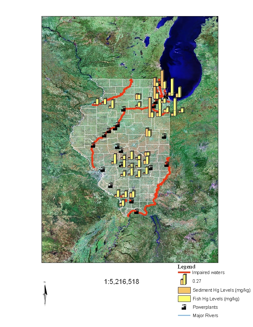
Thus, there is no consistent relationship between total mercury
concentrations in sediments and mercury concentrations (primarily methyl mercury) in
fish tissues of impaired waters.
Power plant locations and Illinois impaired waters are also shown in Figures 2 and 3.
Exceedances of 0.1 and 0.23 ppm total mercury levels in fish were not always found at
sites in close proximity to power plants, nor were impaired waters always associated with
power plants. Moreover, given that the winds in Illinois are primarily south, southwest
and north, northwest in the winter
32
, emissions from power plants do not appear to be
responsible for all waters in Illinois impaired due to mercury (e.g., Rock River). Thus,
there is no clear and consistent relationship between Illinois coal-fired power plants
and methyl mercury concentrations in fish in Illinois waters.
This finding is not
unexpected given the complexity of the global mercury cycle. Although there is no
question that coal-fired power plants are significant sources of mercury to the
atmosphere, they are not the largest sources of mercury deposited in Illinois
33
. These
emissions cannot be directly related to mercury concentrations in fish collected from
30
Illinois EPA, in the TSD, assumes that if mercury is not detected, it is present at 50% of the detection
limits [cf Marcia Willhite’s verbal testimony of June 14, 2006: e.g., at pages 84-85 and pages 158-160 of
the transcript of that testimony]. However, this practice is questionable given that it means that mercury is
assumed to be present when it may not be. Better methods exist for dealing with values below detection
limits: e.g., Shumway RN, Azari RS, Kayhanian M. 2002. Statistical approaches to estimating mean water
quality concentrations with detection limits. Environ Sci Technol 36: 3345-53; also, Helsel DR. 2005.
More than obvious: Better methods for interpreting nondetect data. Environ Sci Technol October 15, 2005:
419A-23A.
31
Clarification regarding the 0.06 and 0.23 ppm mercury values was provided by Dr. Hornshaw in verbal
testimony on June 14, 2006: at pages 25 and 26 of the transcript of that testimony.
32
Gerald Keeler’s verbal testimony of June 15, 2006: at page 32 of the transcript of that testimony.
33
K Vijayaraghavan in his testimony at page 7 estimates “U.S. coal-fired power plants are calculated to
contribute 19% of mercury deposition in Illinois in 2006.”; also, see Section 3.0, page 4 of the present
document (Testimony of Peter M. Chapman)
Page 11
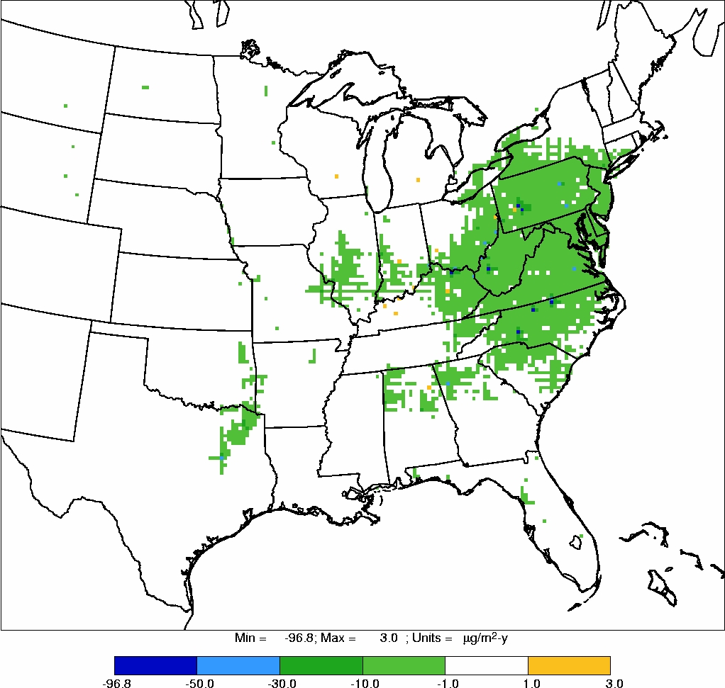
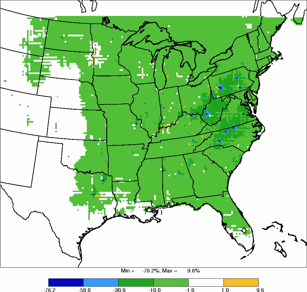
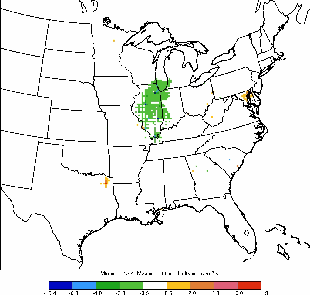
nearby water bodies. Further, Illinois’ proposed rule would only result in a 4% reduction
in depositions in Illinois from Illinois coal-fired power plant mercury emissions
compared to the CAMR
34
, which would likely not result in a measurable decrease in
mercury concentrations in fish in Illinois water bodies compared to the CAMR. As noted
at page 3 of Gerald Keeler’s testimony, “The relationship between the emissions of
mercury to the atmosphere from any one plant and the amount received at any receptor is
complex.” Interestingly, as noted by Thomas Hornshaw in his verbal testimony of
June 16, 2006 (at pages 84-85 of the transcript), Illinois fish tissue mercury levels are
lower than in some other Great Lakes States.
The discussion above explains the “no” answer to Question 1 (Section 2.0). The
discussion below explains the “no” answer to Question 2 (Section 2.0).
The Illinois 2004 Section 303(d) List
35
was reviewed, to identify water bodies considered
impaired by the State due to mercury and/or PCB concentrations. Table 4
36
summarizes
these sites, listing water body name, site name, and whether the site is impaired due to
levels of mercury and/or PCBs. Fifty-five of the 74 sites (74%) in Illinois listed as
impaired due to mercury would continue to be impaired even if full compliance with the
proposed rule were achieved and the projected fish mercury reductions were achieved.
The presence of PCBs renders the proposed rule ineffective at removing impairment
restrictions. Thus, even if fish mercury levels were to drop below the State mercury
threshold for impaired waters, which is highly unlikely as noted previously, the
classification of these sites as impaired would not change.
5.0 Florida, Massachusetts and Ohio Studies: Relevance to Illinois
We have found no published studies that specifically evaluate coal-fired power plant
mercury emissions and trends in methyl mercury levels in fish. The TSD relies on data
from Florida and Massachusetts to support its conclusion that reducing local coal-fired
power plant inorganic mercury emissions will similarly reduce local fish methyl mercury
34
Testimony of K. Vijayaraghavan at page 7.
35
Illinois Environmental Protection Agency, IEPA/BOW/04-005.
36
Source: Appendix A of the IEPA 2004 document.
Page 12
levels. A study in Ohio is also mentioned in testimony by IEPA witness Dr. Keeler,
however complete details of this study (i.e., the full report) have not been provided by
Dr. Keeler.
As noted in the TSD, Massachusetts has implemented mercury reduction programs, but
has not specifically focused on coal-fired power plants. The Massachusetts study
37
monitored mercury concentrations in Largemouth bass (LMB) and yellow perch (YP)
from 1999 to 2004. The authors noted at page viii that “Over this period consistent and
substantial statistically significant decreases in YP and LMB fish tissue mercury
concentrations occurred in most lakes sampled.” However, decreases did not occur in all
lakes (about 24% showed no decreases for YP and about 35% showed no decreases for
LMB), the level of decrease was variable, and there were some inconsistencies (e.g., at
page 7, “an apparent large temporal increase in tissue mercury concentrations between
1999 and 2004” in one lake and “a slight increase over the 1999 value” for 2004 fish
tissue data from another lake). It was estimated (at page viii) that mercury emissions in
the main deposition area identified in the TSD “decreased by about 87% between the late
1990’s and 2004 due to new pollution controls on municipal solid waste combustors
(MSWC) and the closure of medical waste incinerators (MWIs) and a MSWC in the
area.” But there was far from a 1:1 relationship between decreased emissions and
decreased methyl mercury concentrations in fish; in fact, the Massachusetts study
38
concluded that “…significant reductions from out-of-state mercury sources will likely be
needed to achieve water quality and public health objectives in Massachusetts.” The page
and a half in the TSD dedicated to the Massachusetts study provides an overly simplified
summary of this complex study, as does Marcia Willhite’s testimony.
Similarly, the TSD does not deal fully with the Florida study, which is a modeling study
that makes predictions that do not appear to be supported by available data. Marcia
Willhite, in her testimony, also simplifies the findings of the Florida study. Just a few of
37
Massachusetts Dept of Environmental Protection. 2006. Massachusetts Fish Tissue Mercury Studies:
Long-Term Monitoring Results, 1999-2004.
38
Massachusetts Dept of Environmental Protection. 2006. op. cit., at page viii.
Page 13
the caveats noted at page v of the Florida study report include
39
: the major assumption
that all mercury deposited via wet deposition was from local sources which cannot be the
case given global cycling of mercury; the acknowledgment that mercury cycling cannot
yet be fully modelled; and the fact that different areas might respond differently due to
site-specific differences (e.g., different habitat, food web dynamics and water quality). Of
note, Figure 5.7 in the TSD is labeled “Relation between Atmospheric Mercury Load and
Body Burden in Largemouth Bass”, whereas in the original Florida study (Figure 9, at
page 40) it is labelled “Predicted Hg concentrations in age 3 largemouth bass as a
function of different long term constant annual rates of wet and dry Hg(II) deposition.”
The fact this is a prediction rather than reality is not mentioned in the TSD.
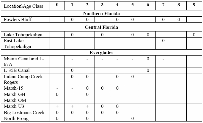
The actual field data reported in the Florida study do show some correlations between
reducing emissions and decreases in methyl mercury concentrations in some biota at
some locations, which is not unexpected. However, the actual data do not show a 1:1
relationship and in some locations show no correlation, which is also not surprising given
the simplifications made by the model which the authors of the Florida study
acknowledge but which the TSD does not mention. There are several examples in the
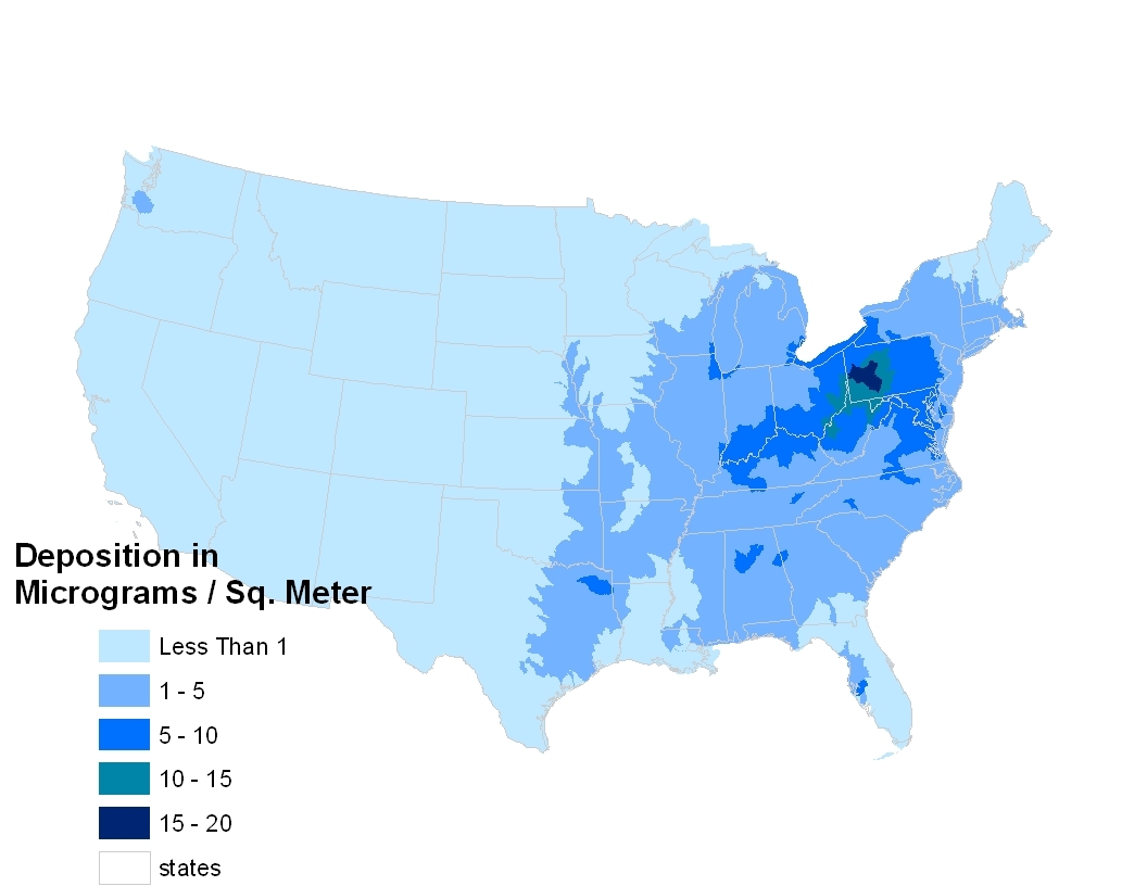
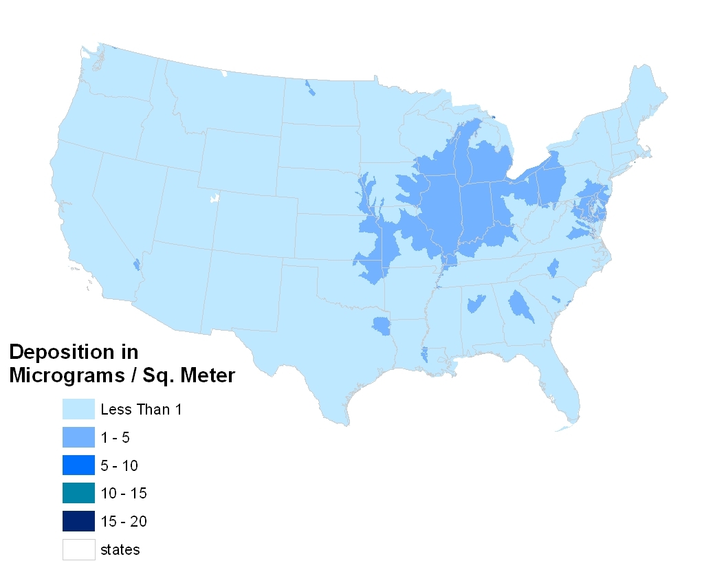
Florida study of differences between the 1:1 prediction and the reality. For example,
although emissions showed a declining trend from 1994 to 2000, mercury wet deposition
for this same time period remained relatively constant (Figure 24 at page 81 of the
Florida study report). The Florida study report at pages 81-82 assessed trends in mercury
concentrations in biota based on levels in Largemouth bass from 12 sites across Florida, 9
of which were in the Everglades and at least 3 of which were in the study area. There
were enough data in only a little over half of the available data sets to conduct statistical
tests for significance. The two sites with the most consistent declines are shown in the
TSD (Figure 5.5, basically the same figure as Figure 25, at page 83 in the Florida study
report). What is not mentioned in the TSD is that there were also examples of no declines
as well as of increases in fish methyl mercury concentrations. In fact, as noted in the
Florida study report (at page 81) and as confirmed by Gerald Keeler in his verbal
testimony on June 15, 2006 (at page 13 of the transcript), about half the cohorts in the
39
Florida Dept of Environmental Protection, op. cit.
Page 14
study area showed no change. The “bottom line” is that, although the Florida modeling
suggests a 1:1 relationship between inorganic mercury emissions and methyl mercury
concentrations in fish, this relationship is not supported by actual data and, given the
simplifications inherent in the model, is highly unlikely to reflect the “real-life” situation.
6.0 Conclusions
At the start of my testimony (Section 2.0) I asked and answered “no” to two key
questions, below:
Question 1:
Will reducing inorganic mercury emissions from coal-fired power plants in
Illinois under the proposed rule reduce organic (methyl) mercury concentrations in fish
living in water bodies in Illinois to the same extent?
Question 2:
Will reducing inorganic mercury emissions from coal-fired power plants in
Illinois under the proposed rule ensure that impairment restrictions can be lifted for
water bodies where fish have elevated mercury concentrations?
The reasons for my answers follow from my detailed testimony above. Reducing
inorganic mercury emissions from coal-fired power plants will result in a decreased level
of inorganic mercury deposition. However, even if reductions in mercury depositions
were to occur in Illinois, reductions in methyl mercury concentrations in local fish will
not occur to the same level as the emission reductions. Mercury is a global problem, not
just a local problem, and the pathways from inorganic mercury emissions to methyl
mercury in fish are complex and governed by site-specific differences that are not readily
predictable
40
. Generalizations such as a 1:1 relationship do not reflect reality.
The
amount of methyl mercury in fish is site specific, as confirmed by Marcia Willhite (see
footnote 18), and is not related simply to the amount of inorganic mercury that is
deposited to a water body.
Moreover, even if mercury levels in Illinois water bodies were
reduced below levels of potential concern, elevated levels of PCBs would still result in an
“impaired” designation for the vast majority of those water bodies.
40
Eisler 2006, op. cit.
Page 15
The goal of the proposed rule, as summarized in Marcia Willhite’s written testimony at
page 4 (“In order to assure that 95% of largemouth bass in Illinois waters may be
consumed in unlimited quantities by sensitive subpopulations, a 90% reduction of
mercury in fish tissue is needed”), will not be achieved.
Page 16
Table 2
Relationship between total mercury concentrations in sediments (mg/kg dry weight) and
fish tissues (mg/kg wet weight). Source: USEPA’s STORET data base. Values represent
sites with fish tissue mercury levels at or above 0.1 mg/kg wet weight. Fish data for the
year referenced; sediment data for samples collected within a 5-year period of the fish
tissue data collection date (2.5 years before and after the date of the tissue collection)
.
Sediment values shown are an average sediment concentration of these 5 years.
County
Total Mercury in Fish Tissue
(mg/kg wet weight)
Total Mercury in
Sediments (mg/kg dry
weight)
Year Fish Data Collected
Jackson
0.185
0.052
1986
Jackson
0.15
0.052
1990
Jackson
0.167
0.115
1988
Jackson
0.167
0.077
1988
Fayette
0.184
0.03
1978
Fayette
0.184
0.04
1978
Fayette
0.13
0.04
1979
Fayette
0.1
0.03
1980
Fayette
0.1
0.035
1980
Fayette
0.205
0.03
1981
Fayette
0.205
0.04
1981
Fayette
0.205
0.035
1981
Fayette
0.205
0.035
1981
Fayette
0.1
0.035
1983
Macoupin
0.26
0.048
1990
Coles
0.21
0.1
1991
Coles
0.1
0.1
1991
Champaign
0.16
0.215
1981
Kankakee
0.12
0.04
1978
Kankakee
0.12
0.05
1978
Kankakee
0.14
0.53
1988
Kankakee
0.14
0.08
1988
Henry
0.22
0.055
1981
La Salle
0.13
0.14
1988
La Salle
0.12
0.029
1990
Henry
0.143
0.037
1978
Henry
0.143
0.03
1978
Cook
0.15
0.331
1974
Cook
0.47
0.061
1990
Cook
0.47
0.1
1990
Cook
0.273
0.1
1991
Cook
0.1
0.221
1990
Cook
0.46
0.091
1991
Cook
0.19
0.49
1981
Page 17
Table 3
Relationship between total mercury concentrations in sediments (mg/kg dry weight) and
fish tissues (mg/kg wet weight). Source: USEPA’s STORET data base. Values represent
sites with fish tissue mercury levels at or above 0.23 mg/kg wet weight. Fish data for the
year referenced; sediment data for samples collected within a 5-year period of the fish
tissue data collection date (2.5 years before and after the date of the tissue collection)
.
Sediment values shown are an average sediment concentration of these 5 years.
COUNTY
Total Mercury in
Sediments (mg/kg
dry weight)
Total Mercury in
Fish Tissue
(mg/kg wet
weight)
Year Fish Data
Collected
Coles
0.113
0.23
1979
Coles
0.113
0.26
1979
Cook
0.49
0.24
1981
Cook
0.49
0.25
1981
Cook
0.49
0.27
1981
Cook
0.49
0.23
1981
Cook
0.061
0.61
1988
Cook
0.074
0.47
1990
Cook
0.1
0.26
1991
Cook
0.1
0.25
1992
Cook
0.1
0.31
1991
Cook
0.1
0.27
1992
Cook
0.221
1.4
1988
Cook
0.091
0.46
1991
Du Page
0.1
0.27
1998
Effingham
0.016
0.4
1989
Effingham
0.018
0.33
1989
Effingham
0.023
0.23
1989
Effingham
0.027
0.29
1989
Effingham
0.029
0.33
1989
Fayette
0.035
0.27
1978
Jackson
0.052
0.25
1986
Macoupin
0.048
0.26
1990
Clay
0.016
0.42
1989
Clay
0.024
0.81
1989
Clay
0.012
0.28
1989
Page 18
Table 4
Summary of current information on waters listed as impaired due to mercury, PCBs, or both as
documented in Appendix A of the Illinois 2004 303(d) List (IEPA/BOW/04-005). IEPA, 2004.
Illinois 2004 Section 303(d) List. Bureau of Water, Watershed Management Section, Planning
Unit. IEPA/BOW/04-005.
Water Body
Site Name
Size
Miles/
Acres
Hg
Impaired?
PCB
Impaired?
Could
Reduction
in Mercury
Affect
Impaired
Listing?
Des Plaines
IL_G-15
3.47 miles
NO
IL_G-22
4.14 miles
NO
IL_G-26
3.32 miles
NO
IL_G-28
8.82 miles
NO
IL_G-30
5.14 miles
NO
IL_G-32
6.08 miles
NO
IL_G-35
5.1 miles
NO
IL_G-36
6.92 miles
NO
IL_G-03
15.08 miles
NO
IL_G-11
5.17 miles
NO
IL_G-23
2.65 miles
NO
IL_G-39
11.12 miles
NO
IL_G-07
10.22 miles
NO
IL_G-08
0.77 miles
YES
IL_G-25
6.78 miles
YES
IL_G-26
3.32 miles
NO
IL_G-01
2.71 miles
NO
IL_G-12
8.35 miles
NO
IL_G-14
4.87 miles
NO
Chicago River
IL_HCB-01
2.56 miles
NO
Devils Kitchen
IL_RNJ
810 acres
YES
Little Grassy
IL_RNK
1000 acres
YES
Campus
IL_RNZH
40 acres
NO
Marquette Park Lagoon
IL_RHE
40 acres
YES
E. BR. DuPage R.
IL_GBL-08
5.53 miles
YES
IL_GBL-10
4.63 miles
YES
Salt Creek
IL_GL
11.19 miles
NO
IL_GL-03
10.38 miles
NO
IL_GL-09
11.78 miles
NO
IL_GL-10
3.64 miles
NO
IL_GL-19
3.1 miles
NO
Page 19
Table 4
Summary of current information on waters listed as impaired due to mercury, PCBs, or both as
documented in Appendix A of the Illinois 2004 303(d) List (IEPA/BOW/04-005). IEPA, 2004.
Illinois 2004 Section 303(d) List. Bureau of Water, Watershed Management Section, Planning
Unit. IEPA/BOW/04-005.
Water Body
Site Name
Size
Miles/
Acres
Hg
Impaired?
PCB
Impaired?
Could
Reduction
in Mercury
Affect
Impaired
Listing?
Cedar (Jackson)
IL_RNE
1800 acres
YES
Calumet-Sag Channel
IL_H-02
10.35 miles
NO
Little Calumet R. N.
IL_HA-05
5.06 miles
NO
Little Calumet R. S.
IL-HB-01
8.6 miles
YES
IL_HB-42
406 miles
YES
Arrowhead (Cook)
IL_RHZE
14 acres
YES
Midlothian Reservoir
IL_RHZI
25 acres
NO
Petticone Creek
IL_QA-C4
0.27 miles
NO
Lake-In-The-Hills 1W
IL_RTZZ
54 acres
YES
Rock River
IL_P-14
10.91 miles
NO
IL_P-20
13.62 miles
NO
IL_P-23
0.96 miles
NO
IL_P-15
21.19 miles
NO
IL_P-06
8.57 miles
NO
IL_P-21
18.36 miles
NO
IL_P-04
19.54 miles
NO
IL_P-06
8.57 miles
NO
IL_P-24
25.18 miles
NO
IL_P-25
15.13 miles
NO
IL_P-09
5.62 miles
NO
Illinois River
IL_D-31
25.49 miles
NO
IL_D-32
13.89 miles
NO
IL_D-16
6.58 miles
NO
IL_D-09
20.09 miles
NO
IL_D-01
35.09 miles
NO
IL_D-20
1.17 miles
NO
IL_D-23
10.52 miles
NO
IL_D-05
12.19 miles
NO
IL_D-10
9.38 miles
NO
IL_D-30
19.92 miles
NO
Page 20
Table 4
Summary of current information on waters listed as impaired due to mercury, PCBs, or both as
documented in Appendix A of the Illinois 2004 303(d) List (IEPA/BOW/04-005). IEPA, 2004.
Illinois 2004 Section 303(d) List. Bureau of Water, Watershed Management Section, Planning
Unit. IEPA/BOW/04-005.
Water Body
Site Name
Size
Miles/
Acres
Hg
Impaired?
PCB
Impaired?
Could
Reduction
in Mercury
Affect
Impaired
Listing?
Kankakee River
IL_F-01
11.54 miles
YES
IL_F-04
10.04 miles
YES
IL_F-12
1.76 miles
YES
IL_F-16
9.57 miles
YES
IL_F-02
13.46 miles
YES
IL_F-03
1.97 miles
YES
Kinkaid
IL_RNC
3475 acres
NO
Wabash River
IL_B-01
4.73 miles
NO
IL_B-06
7.51 miles
NO
IL_B-03
15.21 miles
NO
Monee Reservoir
IL_RFH
46 acres
YES
Big Bureau Creek
IL_DQ-03
5.31 miles
NO
Bracken
IL_SDZA
172 acres
NO
Page 21
Figure 2
Mercury Methylation
Figure 1
The Mercury Cycle
Page 22
Figure 3
Relationship Between Total Mercury Concentrations in Sediments (mg/kg dry
weight) and Fish Tissue Concentrations (mg/kg wet weight) Greater Than or
Equal to 0.1 and Their Proximity to Listed Impaired Waters and Coal-Fired
Power Plants in Illinois.
Note: the information plotted comprises locations with
sediment and tissue data collected from the same site within a 5-year period.
Scale 1: 5,216,518
Page 23
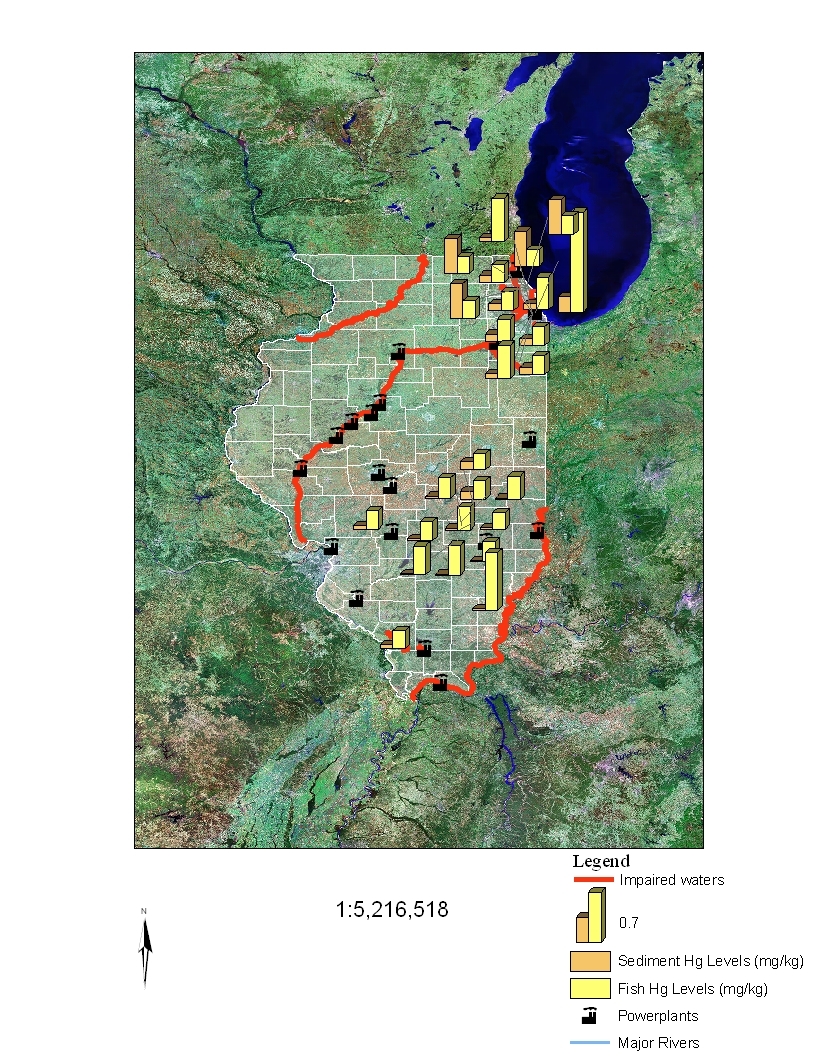
Figure 4
Relationship Between Total Mercury Concentrations in Sediments (mg/kg dry weight) and Fish
Tissue Concentrations (mg/kg wet weight) Greater Than or Equal to 0.23 and Their Proximity to
Listed Impaired Waters and Coal-Fired Power Plants in Illinois.
Note: the information plotted
comprises locations with sediment and tissue data collected from the same site within a 5-year period.
Scale 1: 5,216,518
Page 24
Education:
Ph.D., Benthic Ecology, University of Victoria, Victoria, BC, 1979
M.Sc., Biological Oceanography, 1976
B.Sc., Marine Biology, 1974
Affiliations:
Member, American Water Works Association
Member, North American Benthological Society
Member, American Society for Testing and Materials
Charter Member, Estuarine Research Federation
Member, Society of Environmental Toxicology and Chemistry (SETAC)
Member, Water Environment Federation
Awards:
Founders Award, Society of Environmental Toxicology and Chemistry, 2001
Region 10 award for resolving environmental issues, Port Valdez, Alaska, 1996
Languages:
English and Spanish
Publications:
Over 150 journal articles and book chapters
Over 200 technical reports
Over 100 presentations at meetings
Experience:
2004 – Present
Golder Associates Ltd.
North Vancouver, BC
Senior Environmental Scientist, Principal
Responsibilities include directing, designing, and managing environmental studies in
Arctic, temperate, and tropical ecosystems. Primary areas of expertise and
responsibilities are in ecotoxicology, risk assessment, and aquatic ecology. Areas of
specialisation include weight of evidence assessments and metals fate and effects,
especially selenium.
1979 – 2004
EVS Environmental Consultants
North Vancouver, BC
Senior Environmental Scientist/Principal
Responsibilities included directing, designing, and managing environmental studies in
Arctic, temperate, and tropical ecosystems. Primary areas of expertise and
responsibilities were ecotoxicology, risk assessment, and aquatic ecology. Areas of
specialisation included weight of evidence assessments and metals.
1977 – 1979
Environment Canada/Dept. Fisheries and Oceans
Victoria, BC
Independent Contractor
Conducted independent research on aquatic oligochaete distributions in the Fraser
River and assessed metal body burdens in aquatic benthos from various areas.
Published several papers and one book chapter based on this work.
1976 – 1979
University of Victoria
Victoria, BC
Teaching and Research Assistant
Prepared laboratories for undergraduate classes and provided lectures during
laboratory classes. Involvement in research activities included species collections
(terrestrial and aquatic), laboratory and field studies.
ECOTOXICOLOGY/TOXICITY TESTING Page 1 of 1
PROJECT RELATED EXPERIENCE – ECOTOXICOLOGY/TOXICITY
TESTING
Ecotoxicology
North and South America, Europe, Australasia
•
Directed development and source evaluation studies of chemical contaminants in water and
sediment.
•
Designed, directed and conducted studies involving sewage treatment plants, mining,
manufacturing, pulp and paper, wood processing, hazardous waste disposal, landfill operations, oil
and gas, smelting and food processing.
•
Conducted pioneering toxicity studies in Arctic, temperate, and tropical ecosystems.
Toxicity Testing
North and South America, Europe, Australasia
•
Nationally and internationally recognised expert in ecotoxicology.
•
Developed
and
verified
national
and
international
bioassessment
protocols
for
measuring/predicting toxicity and bioaccumulation.
Example Publications
International Peer-Reviewed Literature
Chapman, P.M. and J. Anderson. 2005. A decision-making framework for sediment contamination. Integr.
Environ. Assess. Manage. 1: 163-173.
Chapman, P.M. and M.J. Riddle. 2005. Toxic effects of contaminants in polar marine environments.
Environ. Sci. Technol. 38: 200A-207A.
Wang, F., R. Goulet, and P.M. Chapman. 2004. A critique of testing sediment biological effects with the
freshwater amphipod
Hyalella azteca
. Chemosphere 57: 1713-1724.
McDonald, B.G. and P.M. Chapman. 2002. PAH phototoxicity – An ecologically irrelevant phenomenon?
Mar. Pollut. Bull. 44: 1321-1326.
Chapman, P.M., H. Bailey, and E. Canaria. 2000. Toxicity of total dissolved solids (TDS) from two mine
effluents to chironomid larvae and early life stages of rainbow trout. Environ. Toxicol. Chem. 19:
210-214.
Wang, F. and P.M. Chapman. 1999. The biological implications of sulfide in sediment - a review focusing
on sediment toxicity. Environ. Toxicol. Chem. 18: 2526-2532.
Chapman, P.M. 1998. New and emerging issues in ecotoxicology - the shape of testing to come? Austral.
J. Ecotox. 4:1-7.
Chapman, P.M. 1997. Acid volatile sulfides, equilibrium partitioning, and hazardous waste site sediments.
Environ. Manage. 21: 197-202.
Chapman, P.M. 1990. The Sediment Quality Triad approach to determining pollution-induced degradation.
Sci. Tot. Environ. 97-8: 815-825.
ENVIRONMENTAL RISK ASSESSMENT
Page 1 of 2
PROJECT RELATED EXPERIENCE – ENVIRONMENTAL RISK
ASSESSMENT
Various Projects
North and South America, Europe, Australasia
•
Involved in ecological risk assessment since this process was formalised in the 1980s.
•
Conducted ecological risk assessments for government and industry.
•
Served, at the request of the U.S. Environmental Protection Agency Risk Assessment Forum, as a
peer reviewer for various agency guidance documents.
•
Published extensively on ecological risk assessment.
Global Experience
South America, Europe, Australasia
•
Senior Editor of the international peer-reviewed journal, Human and Ecological Risk Assessment.
•
Advisory and consulting services to the governments of Australia, Peru, Indonesia, Hong Kong,
ASEAN (Association of South East Asian Nations).
•
Helped set up the first Master’s degree in Ecotoxicology in Portugal.
•
Conducted pioneering toxicity testing studies in the Arctic, North Sea, and Venice lagoons.
•
Lectured, taught, and worked extensively in Europe, South East Asia, Australia, and South
America (fluent in Spanish).
•
Independent, external examiner for Ph.D. dissertations in Spain, Finland, Canada, the U.S.,
Denmark, and Australia.
•
Numerous lectures and presentations to the public, high school and university classes, business
and professional groups.
Large-Project Expertise
North and South America, Europe, Australasia
•
Responsible for synthesis of all studies conducted through NSERC (Natural Sciences and Engineering
Research Council) under the Metals in the Environment Research Network (MITE-RN; www.mite-
rn.org). MITE-RN ran for 5 years and involved 7 major Canadian Universities and over 20 Principal
Investigators from those Universities plus graduate students and other collaborators.
•
Currently providing similar services to the successor of MITE-RN, the Metals in the Holistic
Environment Research Network (MITHE-RN); www.mithe-rn.org
.
•
Directed regional-scale risk assessments in Alaska (Port Valdez), Papua New Guinea, Irian Jaya,
Chile, and Peru.
Example Publications
International Peer-Reviewed Literature
Campbell, P.G.C., P.M. Chapman, and B. Hale. 2006. Risk assessment of metals in the environment. pp
102-131, In: Hester, R. E. and R. M. Harrison (eds.), Chemicals in the Environment: Assessing and
Managing Risk. Issues in Environmental Science and Technology Volume 22, Royal Society of
Chemistry, Cambridge, UK.
Chapman, P.M., F. Wang, C. Janssen, R.R. Goulet, and C.N. Kamunde. 2003. Conducting ecological risk
assessments of inorganic metals and metalloids – Current status. Human Ecol Risk Assess 9: 641-697.
[This paper was selected as the Ecological Risk Assessment Paper of the Year 2003]
Chapman, P.M., B.G. McDonald, and G.S. Lawrence. 2002. Weight of evidence frameworks for sediment
quality and other assessments. Human Ecol. Risk Assess. 8: 1489-1515.
Chapman, P.M. 2002. Ecological risk assessment (ERA) and hormesis. Sci. Tot. Environ.288: 131-140.
ENVIRONMENTAL QUALITY MGT/AQUATIC ECOLOGY Page 1 of 2
PROJECT RELATED EXPERIENCE – ENVIRONMENTAL QUALITY
MANAGEMENT/AQUATIC POLLUTION ASSESSMENT
Environmental Quality
North and South America, Europe, Australasia, Arctic
•
Intimately involved in the process and methods for developing environmental quality guidelines,
both nationally and internationally.
•
Advisor to the federal governments of both the United States and Canada for environmental
toxicology and biomonitoring assessment policy and protocols.
•
Participated in and led aspects of international (South American, European, and Australasian)
monitoring development projects.
•
Published extensively on the subject of environmental quality guidelines.
•
Member of the International Standards Organization, representing Canada.
Pollution Assessment
North and South America, Europe, Australasia, Arctic
•
Developed the internationally recognised and accepted Sediment Quality Triad concept for
determining pollution-induced degradation in aquatic habitats.
•
Directed projects (for government and industry) for various studies involving biological
monitoring; assessment of toxicant levels (including Priority Pollutants) in tissues, sediments, and
water; ecological surveys; literature reviews for ranking environmental contaminants; and
bioassessment (e.g., toxicity testing).
Dredging/Sediment Projects
USA, Canada, and elsewhere
•
Peer reviewed the U.S. Environmental Protection Agency/Army Corps of Engineers
[USEPA/USACE] “Green Book” on ocean disposal.
•
Contracted author for the EPA/USACE Inland Testing Manual for Waters of the U.S.
•
Designed and implemented monitoring and assessment projects for aquatic dredging in fresh,
marine, and estuarine waters world-wide.
Example Publications
International Peer-Reviewed Literature
Chapman, P.M., W.S. Douglas, M.C. Harrass, R.M. Burgess, D.D. Reible, W.H. Clements, A.H.
Ringwood, C. Hogstrand, and W.J. Birge. 2005. Workgroup summary report on the role of SQGs and
other tools in different aquatic habitats. In: Wenning, R., C. Ingersoll, G. Batley, and M. Moore (eds.),
Use of Sediment Quality Guidelines (SQGs) and Related Tools for the Assessment of Contaminated
Sediments. SETAC Press, Pensacola, FL, USA.
Chapman, P.M., F. Wang, D.D. Germano, and G. Batley. 2002. Porewater testing and analysis: The good,
the bad and the ugly. Mar. Pollut. Bull. 44: 359-366.
Chapman, P.M. 2001. Utility and relevance of aquatic oligochaetes in ecological risk assessment.
Hydrobiologia 463:149-169.
Chapman, P.M., F. Wang, W. Adams, and A. Green. 1999. Appropriate uses of sediment quality values for
metals and metalloids. Environ. Sci. Technol. 33: 3937-3941.
Chapman, P.M., P.J. Allard, and G.A. Vigers. 1999. Development of sediment quality values for Hong
Kong Special Administrative Region: a possible model for other jurisdictions. Mar. Pollut. Bull. 38:
161-169.
EXPERT WITNESS AND PEER REVIEW
Page 1 of 1
PROJECT RELATED EXPERIENCE – EXPERT WITNESS AND PEER
REVIEW
Expert Witness
USA and Canada
•
Four trials with testimony.
•
Two trials with attendance but no testimony as cases settled.
•
Two depositions (one videotaped).
•
One pending trial.
•
Appeared as an expert witness on eight occasions before the Northwest Territories (Canada) Water
Board, and on one occasion before the Nunavut (Canada) Water Board.
•
Provided expert advice, but not testimony, during five judicial or quasi-judicial Hearings in
Canada.
•
Clients include both government (e.g., U.S. Department of Justice) and industry.
Peer Reviewer
USA, Canada, Australasia, Europe
Currently:
•
Peer reviewer for over 20 international scientific journals.
•
Peer reviewer for American, Canadian, Australian, New Zealand, and European granting agencies.
•
Senior Editor for Debates/Commentaries and Perspectives for the international, peer-reviewed
journal, Human and Ecological Risk Assessment.
•
Editor of the Learned Discourses in the Society of Environmental Toxicology and Chemistry
(SETAC) Globe.
•
Editorial Board of the international journal, Marine Pollution Bulletin.
•
Editorial Board of the international journal, Environmental Toxicology and Chemistry.
Previously:
•
Member, U.S. Environmental Protection Agency, Science Advisory Board (SAB), Sediment
Criteria Subcommittee.
•
Member, Washington State Biomonitoring Science Advisory Board (BSAB).
•
Member, Canadian Environmental Advisory Council (advised four different Canadian Ministers
of Environment).
•
Member, NRC Committee on the Bioavailability of Metals in Sediments.
•
Member, U.S. Environmental Protection Agency, Science Advisory Board, Global Climate
Change Subcommittee.
•
Member, Editorial Board, Chemosphere.
•
Member, Sewage Treatment Review Panel.
•
Member, International Technical Advisory Panel on Ecotoxicity.
METALS AND METALLOIDS Page 1 of 1
PROJECT RELATED EXPERIENCE – METALS AND METALLOIDS
Metals and Metalloids
North and South America, Europe, Australasia, Arctic
•
Past member of the International Technical Advisory Panel on Ecotoxicology, for nonferrous
metals.
•
Participated in an OECD Expert Workshop on Toxicity Testing of Metals and Metalloids as Chair
of an International Expert Group.
•
Participated in a Canada/European Union Expert Workshop on Persistence and Bioaccumulation
of Metals and Metalloids as a speaker and workshop rapporteur.
•
Participated in a World Health Organization Expert Workshop on Global Criteria for Zinc.
•
Extensive experience and expertise with metals from sources including mining, smelters, sewage,
and landfills.
•
Extensive publications regarding metals fate and effects in the environment.
Example Publications
International Peer-Reviewed Literature
Adams, W. and P.M. Chapman (eds.), 2005. Assessing the Hazard of Metals and Inorganic Metal
Substances in Aquatic and Terrestrial Systems. SETAC Press, Pensacola, FL.
Chapman, P.M. 2005. Inorganic metals and metalloids ERA – Recent advances and implications for LCIA.
pp. 214-219. In: A.A. Dubreuil (ed.), Life Cycle Assessment of Metals – Issues and Research
Directions. SETAC Press, Pensacola, FL.
Chapman, P.M. and C. McPherson. 2004. Possible selenium thresholds for trout. SETAC Globe 5(6):
22-25.
Chapman, P.M. and F. Wang. 2000. Issues in ecological risk assessment of inorganic metals and
metalloids. Human Ecol. Risk Assess. 6: 965-988.
McPherson, C.A. and P.M. Chapman. 2000. Copper effects on potential sediment test organisms: the
importance of appropriate sensitivity. Mar. Pollut. Bull. 40:656-665.
Chapman, P.M. 1999. Selenium - a potential time bomb or just another contaminant? Human Ecol. Risk
Assess. 5: 1122-1137.
Wang, F., P.M. Chapman, and H. Allen. 1999. Misapplication of equilibrium partitioning coefficients to
derive metals sediment quality values. Mar. Pollut. Bull. 38: 423-425.
Chapman, P.M., F. Wang, C. Janssen, G. Persoone, and H. Allen. 1998. Ecotoxicology of metals in aquatic
sediments: binding and release, bioavailability, hazard, risk and remediation. Can. J. Fish. Aquat. Sci.
55: 2221-2243.
Chapman, P.M., H.E. Allen, K. Godtfredsen, and M.N. Z’Graggen. 1996. Evaluation of BCFs as measures
for classifying and regulating metals. Environ. Sci. Technol. 30: 448-452.
SEWAGE EFFLUENT AND TREATMENT
Page 1 of 1
PROJECT RELATED EXPERIENCE – SEWAGE EFFLUENT AND
TREATMENT
Sewage
North and South America, Europe, Australasia, Arctic
•
Extensive project experience assessing fate and effects of sewage effluents.
•
Evaluations for cities with populations over 1,000,000 and small local discharges.
•
Expert advice regarding design and placement of sewage discharges to minimise environmental
concerns.
•
Expert advice regarding levels of sewage treatment required relative to the receiving environment.
•
Interpretative advice and studies regarding environmental effects and regulatory requirements.
•
Member, Sewage Treatment Review Panel (Greater Vancouver Regional District).
Example Publications
International Peer-Reviewed Literature
Chapman, P.M. 2006. Determining when contamination is pollution – weight of evidence determinations
for sediments and effluents. Environ. Intern. (in press).
Chapman, P.M., K. Ho, W. Munns, K. Solomon, and M.P. Weinstein. 2002. Issues in sediment toxicity and
ecological risk assessment. Mar. Pollut. Bull. 44: 271-278.
McPherson, C.A., A.R. Tang, P.M. Chapman, and L.A. Taylor. 2002. Toxicity of 1,4-dichlorobenzene in
sediments to juvenile polychaete worms. Mar. Pollut. Bull. 44: 1405-1414.
Chapman, P.M. 2000. Whole Effluent Toxicity (WET) Testing - usefulness, level of protection, and risk
assessment. Environ. Toxicol. Chem. 19: 3-13.
Taylor, L.A., P.M. Chapman, R.A. Miller, and R.V. Pym. 1998. The effects of untreated municipal sewage
discharge to the marine environment off Victoria, British Columbia, Canada. Water Sci. Technol. 38:
285-292.
McGroddy, S. and P.M. Chapman. 1997. Is mercury from dental amalgam an environmental problem?
Environ. Toxicol. Chem. 16: 2213-2214.
Chapman, P.M., J. Downie, A. Maynard, and L. Taylor. 1996. Deodorizer residue and coal in marine
sediments contaminants or pollutants? Environ. Toxicol. Chem. 15: 638-642.
Chapman, P.M., M.D. Paine, A.D. Arthur, and L.A. Taylor. 1996. A triad study of sediment quality
associated with a major, relatively untreated marine sewage discharge. Mar. Pollut. Bull. 32: 47- 64.
Chapman, P.M. 1996. A test of sediment effects concentrations: DDT and PCB in the Southern California
Bight. Environ. Toxicol. Chem. 15: 1197-1198.
Chapman, P.M., A.D. Arthur, M.D. Paine, and L.A. Taylor. 1994. Sediment studies provide key
information on the need to treat sewage discharged to sea by a major Canadian city. Water Sci.
Technol. 28: 255-261.
JOURNAL PUBLICATIONS Page 1 of 9
JOURNAL PUBLICATIONS
[* = Editorials or Letters to the Editor]
Chapman, P.M., C. McPherson, and C. MacCay. In Preparation. Greater contamination and effects pre-
than post-mining: a case study. Arch. Environ. Contam. Toxicol.
Lofts, S., P. M. Chapman, I. Schoeters, R. Dwyer, S. Sheppard, M. McLaughlin, et al. In Preparation.
Appropriate critical loads of metals to terrestrial environments. Environ. Sci. Technol.
Liber, K., M.D. Paine, C.A. McPherson, B.S. Kelemen, P.M. Chapman, and I.K. Birtwell. In Preparation.
Effects of suspended placer mining sediment on juvenile Chinook salmon and arctic grayling embryos
in experimental systems. Can. J. Fish. Aquati. Sci.
Chapman, P. M. In press. Future environmental science: “Status humana”, man as the measure. Human
Ecol. Risk Assess.
Chapman, P.M. In press. Determining when contamination is pollution - weight of evidence determinations
for sediments and effluents. Environ. Intern.
Chapman, P.M., B. McDonald, P.E. Kickham, and S. McKinnon. In Press. Global geographic differences
in marine metals toxicity. Mar. Pollut. Bull.
McDonald, B. G. and P. M. Chapman. 2006. Assessing selenium effects: A weight of evidence approach.
Integr. Environ. Assess. Manag. (in press).
*Chapman, P. M. 2006. When is peer review excessive? Examples from peer review Hell. Human Ecol.
Risk Assess. 12: 423-426.
Joillet, O., R. Rosenbaum, P. M. Chapman, T. McKone, M. Margnia, M. Scheringer, N. van Straalen, and
F. Waniah. 2006. Establishing a framework for Life Cycle Toxicity Assessment: Findings of the
Lausanne review workshop. Int. J. Life Cycle Assess. 11: 209-212.
*Chapman, P. M. 2006. Emerging chemicals – emerging problems? Environ. Toxicol. Chem. 25: 1445-
1447.
Chapman, P. M. and Hollert, H. 2006. Should the Sediment Quality Triad become a tetrad, a pentad, or
possibly even a hexad? J Soil Sed 6: 4-8.
*Calado, R. and P. M. Chapman. 2006. Aquarium species: deadly invaders. Mar. Pollut. Bull. 52: 599-601.
*Chapman, P.M. and L.M. Guerra. 2005. The “So what?” factor. Mar. Pollut. Bull. 50: 1457-1458.
Chapman, P.M., R.R. Goulet, and F. Wang. 2005. Response to Borgmann et al. (2005) – sediment toxicity
testing with
Hyalella azteca
. Chemosphere 61: 1744-1745.
Chapman, P.M. and M.J. Riddle. 2005. Polar marine toxicology – future research needs. Mar. Pollut. Bull.
50: 905-908.
Chapman, P.M. and J. Anderson. 2005. A decision-making framework for sediment contamination. Integr.
Environ. Assess. Manage. 1: 163-173.
JOURNAL PUBLICATIONS Page 2 of 9
Chapman, P.M. and M.J. Riddle. 2005. Toxic effects of contaminants in polar marine environments.
Environ. Sci. Technol. 38: 200A-207A.
Wang, F., R. Goulet, and P.M. Chapman. 2004. A critique of testing sediment biological effects with the
freshwater amphipod
Hyalella azteca
. Chemosphere 57: 1713-1724.
*Chapman, P.M. and M.J. Riddle. 2004. Reply to Wells: there really is a paucity of polar marine
ecotoxicity data! Mar. Pollut. Bull. 48: 606-607.
*Chapman, P.M. 2004. Indirect effects of contaminants. Mar. Pollut. Bull. 48: 411-412.
Chapman, P.M. 2004. Modifying Paracelsus’ dictum for sediment quality (and other) assessments. Aquat.
Ecosyst. Health Manage. 7(3): 1-6.
*Riddle, M.J. and P.M. Chapman. 2004. Polar ecotoxicology – a missing link. Antarctic Sci. 15(3):317.
*Wells, P., J. Baker, P.M. Chapman, M. Elliott, P. Hutchings, K. Mann, P. Olive, J. Pearce, D. Phillips, and
C. Sheppard. 2003. From mimeos to e-copy – a tribute to Professor R.B. (Bob) Clark, founding editor
of the
Marine Pollution Bulletin
. Mar. Pollut. Bull. 46: 1051-1054.
*Chapman, P.M. and R.C. Loehr. 2003. Relevant environmental science. Environ. Toxicol. Chem. 22:
2217-2218.
*Chapman, P.M. and M.J. Riddle. 2003. Missing and needed: polar marine ecotoxicology. Mar. Pollut.
Bull. 46:927-928.
Chapman, P.M., F. Wang, C. Janssen, R.R. Goulet, and C.N. Kamunde. 2003. Conducting ecological risk
assessments of inorganic metals and metalloids – Current status. Human Ecol Risk Assess 9: 641-697.
[This paper was selected as the Ecological Risk Assessment Paper of the Year 2003]
McPherson, C.A., A.R. Tang, P.M. Chapman, and L.A. Taylor. 2002. Toxicity of 1,4-dichlorobenzene in
sediments to juvenile polychaete worms. Mar. Pollut. Bull. 44: 1405-1414.
McDonald, B.G. and P.M. Chapman. 2002. PAH phototoxicity – An ecologically irrelevant phenomenon?
Mar. Pollut. Bull. 44: 1321-1326.
Chapman, P.M., B.G. McDonald, and G.S. Lawrence. 2002. Weight of evidence frameworks for sediment
quality and other assessments. Human Ecol. Risk Assess. 8: 1489-1515.
Grapentine, L., J. Anderson, D. Boyd, G.A. Burton, C. De Barros, G. Johnson, C. Marvin, D. Milani, S.
Painter, T. Pascoe, T. Reynoldson, L. Richman, K. Solomon, and P.M. Chapman. 2002. A decision-
making framework for sediment assessment developed for the Great Lakes. Human Ecol. Risk Assess.
8: 1641-1655.
Burton, G.A.Jr., P.M. Chapman, and E.P. Smith. 2002. Weight of evidence approaches for assessing
ecosystem impairment. Human Ecol. Risk Assess. 8: 1657-1673.
Burton, G.A. Jr., G.E. Batley, P.M. Chapman, V.E. Forbes, C.E. Schlekat, P.E. Smith, P.J. den Besten, J.
Barker, T. Reynoldson, A.S. Green, R.L. Dwyer, and W.R. Berti. 2002. A weight of evidence
JOURNAL PUBLICATIONS Page 3 of 9
framework for assessing sediment (or other) contamination: Improving certainty in the
decision-making process. Human Ecol. Risk Assess. 8: 1675-1696.
*Chapman, P.M. and C. Sheppard. 2002. Letters to the editor. Mar. Pollut. Bull. 44: 577-578.
*Chapman, P.M. 2002. Mistakes made/lessons learned. Environ. Toxicol. Chem. 21: 891-893.
Batley, G.E., G.A. Burton, P.M. Chapman, and V.E. Forbes. 2002. Uncertainties in sediment quality
weight-of-evidence (WOE) assessments. Human Ecol. Risk Assess. 8: 1517-1547.
Chapman, P.M., K. Ho, W. Munns, K. Solomon, and M.P. Weinstein. 2002. Issues in sediment toxicity and
ecological risk assessment. Mar. Pollut. Bull. 44: 271-278.
Chapman, P.M. 2002. Defining hormesis - Comments on Calabrese and Baldwin (2002). BELLE
Newsletter 10(2):31-33.
Chapman, P.M., F. Wang, D.D. Germano, and G. Batley. 2002. Porewater testing and analysis: The good,
the bad and the ugly. Mar. Pollut. Bull. 44: 359-366.
Chapman, P.M. 2002. Ecological risk assessment (ERA) and hormesis. Sci. Tot. Environ.288: 131-140.
Chapman, P.M. 2002. Integrating toxicology and benthic ecology: Putting the eco back into ecotoxicology.
Mar. Pollut. Bull. 44: 7-15.
*Chapman, P.M. 2001. How toxic is toxic? Mar. Pollut. Bull. 42: 1279-1280.
Chapman, P.M. 2001. Utility and relevance of aquatic oligochaetes in ecological risk assessment.
Hydrobiologia 463:149-169.
Chapman, P.M. 2001. Final comments: Implications of hormesis to ecotoxicology and ecological risk
assessment (ERA). BELLE Newsletter 10 (1):23-25 and
Human Exp. Toxicol. 20:529-531.
Chapman, P.M. 2001.The implications of hormesis to ecotoxicology and ecological risk assessment.
BELLE Newsletter 10 (1): 2-8 and
Human Exp. Toxicol. 20:499-505.
Chapman, P.M. 2001. Reflections on the future of hormesis. Critical Rev. Toxicol. 31 (4&5): 649-657.
Chapman, P.M. and F. Wang. 2001 Assessing sediment contamination in estuaries. Environ. Toxicol.
Chem. 20: 3-22.
Chapman, P.M. 2000. The Sediment Quality Triad (SQT) - then, now and tomorrow. Int. J. Environ. Pollut.
13:351-356.
Hill, R.A., P.M. Chapman, G.S. Mann, and G.S. Lawrence. 2000. Ecological risk assessments. Soil and
Groundwater Cleanup October/November :12-16.
Chapman, P.M. and F. Wang. 2000. Issues in ecological risk assessment of inorganic metals and
metalloids. Human Ecol. Risk Assess. 6: 965-988.
JOURNAL PUBLICATIONS Page 4 of 9
McPherson, C.A. and P.M. Chapman. 2000. Copper effects on potential sediment test organisms: the
importance of appropriate sensitivity. Mar. Pollut. Bull. 40:656-665.
Hill, R.A., P.M. Chapman, G.L. Mann, and G.S. Lawrence. 2000. Level of detail in ecological risk
assessments. Mar. Pollut. Bull. 40: 471-477.
*Chapman, P.M. 2000. Why are we still emphasizing screening level numbers? Mar. Pollut. Bull.
40:465-466.
Chapman, P.M. 2000. Whole Effluent Toxicity (WET) Testing - usefulness, level of protection, and risk
assessment. Environ. Toxicol. Chem. 19: 3-13.
Chapman, P.M., H. Bailey, and E. Canaria. 2000. Toxicity of total dissolved solids (TDS) from two mine
effluents to chironomid larvae and early life stages of rainbow trout. Environ. Toxicol. Chem. 19:
210-214.
Chapman, P.M., F. Wang, W. Adams, and A. Green. 1999. Appropriate uses of sediment quality values for
metals and metalloids. Environ. Sci. Technol. 33: 3937-3941.
Chapman, P.M. 1999. Selenium - a potential time bomb or just another contaminant? Human Ecol. Risk
Assess. 5: 1122-1137.
*Chapman, P.M. 1999. Conflict of interest rules. Mar. Pollut. Bull. 38: 745-747.
Wang, F. and P.M. Chapman. 1999. The biological implications of sulfide in sediment - a review focusing
on sediment toxicity. Environ. Toxicol. Chem. 18: 2526-2532.
Chapman, P.M. 1999. Risk assessment and the precautionary principle: a time and a place. Mar. Pollut.
Bull. 38: 944-947.
Chapman, P.M. and G.S. Mann. 1999. Sediment quality values (SQVs) and ecological risk assessment
(ERA). Mar. Pollut. Bull. 38: 339-344.
Wang, F., P.M. Chapman, and H. Allen. 1999. Misapplication of equilibrium partitioning coefficients to
derive metals sediment quality values. Mar. Pollut. Bull. 38: 423-425.
Chapman, P.M., P.J. Allard, and G.A. Vigers. 1999. Development of sediment quality values for Hong
Kong Special Administrative Region: a possible model for other jurisdictions. Mar. Pollut. Bull. 38:
161-169.
Chapman, P.M. 1998. New and emerging issues in ecotoxicology - the shape of testing to come? Austral. J.
Ecotox. 4:1-7.
*Chapman, P.M. 1998. Detection limits and biological effects. Mar. Pollut. Bull. 36: 758-759.
Chapman, P.M., F. Wang, C. Janssen, G. Persoone, and H. Allen. 1998. Ecotoxicology of metals in aquatic
sediments: binding and release, bioavailability, hazard, risk and remediation. Can. J. Fish. Aquat. Sci.
55: 2221-2243.
JOURNAL PUBLICATIONS Page 5 of 9
Taylor, L.A., P.M. Chapman, R.A. Miller, and R.V. Pym. 1998. The effects of untreated municipal sewage
discharge to the marine environment off Victoria, British Columbia, Canada. Water Sci. Technol. 38:
285-292.
DelValls, T.A. and P.M. Chapman.1998. Site-specific sediment quality values in the Gulf of Cadiz (Spain)
and in San Francisco Bay (USA) using the sediment quality triad and multivariate analysis. Ciencias
Marinas 24: 313-336.
Chapman, P.M., A. Fairbrother, and D. Brown. 1998. A critical evaluation of safety (uncertainty) factors
for ecological risk assessment. Environ. Toxicol. Chem.17: 99-108.
*Chapman, P.M. and J. Giddings. 1997. Scientists need good manners and to be scientists. Mar. Pollut.
Bull. 11: 852.
Chapman, P.M., P. Anderson, S. Carr, V. Engle, R. Green, J. Hameedi, M. Harmon, P. Haverland, J.
Hyland, C. Ingersoll, E. Long, J. Rodgers Jr., M. Salazar, P.K. Sibley, P.J. Smith, P.C. Swartz, B.
Thompson, and H. Windom. 1997. General guidelines for using the Sediment Quality Triad. Mar.
Pollut. Bull. 34: 368-372.
McGroddy, S. and P.M. Chapman. 1997. Is mercury from dental amalgam an environmental problem?
Environ. Toxicol. Chem. 16: 2213-2214.
Murdoch, M.H., P.M. Chapman, D.M. Johns, and M.D. Paine. 1997. Chronic effects of organochlorine
exposure in sediment to the marine polychaete
Neanthes arenaceodentata
. Environ. Toxicol. Chem.16:
1494-1503.
Murdoch, M.H., P.M. Chapman, D.M. Norman, and V.M. Quintino. 1997. Spiking sediment with
organochlorine
compounds
for
toxicity
testing.
Environ.
Toxicol.
Chem.
16:1504-1509.
*Chapman, P.M. 1997. Is bioaccumulation useful for predicting impacts? Mar. Pollut. Bull. 34: 282-283.
Chapman, P.M. 1997. The Precautionary Principle and ecological quality standards/objectives. Mar. Pollut.
Bull. 34: 227-228.
Chapman, P.F. and P.M. Chapman. 1997. Second Warning! NOECs are inappropriate for regulatory use.
Environ. Toxicol. Chem. 16: 125-126.
Chapman, P.M. 1997. Acid volatile sulfides, equilibrium partitioning, and hazardous waste site sediments.
Environ. Manage. 21: 197-202.
Paine, M.D., P.M. Chapman, P.J. Allard, M.H. Murdoch, and D. Minifie. 1996. Limited bioavailability of
sediment PAH near an aluminum smelter: contamination does not equal effects. Environ. Toxicol.
Chem. 15: 2003-2018.
Chapman, P.M., H.E. Allen, K. Godtfredsen, and M.N. Z’Graggen. 1996. Evaluation of BCFs as measures
for classifying and regulating metals. Environ. Sci. Technol. 30: 448-452.
Chapman, P.M., I. Thornton, G. Persoone, C. Janssen, K. Godtfredsen, and M.N. Z’Graggen. 1996.
International harmonization related to persistence and bioavailability. Human Ecol. Risk Assess. 2:
393-404.
JOURNAL PUBLICATIONS Page 6 of 9
Chapman, P.M., J. Bridgman, J. Kitegawa, D. Dickason, and A. Dailey. 1996. Science and common sense
in Port Valdez, Alaska. Mar. Pollut. Bull. 3-2: 254-256.
Chapman, P.M. 1996. Presentation and interpretation of Sediment Quality Triad data. Ecotoxicology 5:
327-339.
Chapman, P.M. 1996. A test of sediment effects concentrations: DDT and PCB in the Southern California
Bight. Environ. Toxicol. Chem. 15: 1197-1198.
Chapman, P.M., J. Downie, A. Maynard, and L. Taylor. 1996. Deodorizer residue and coal in marine
sediments contaminants or pollutants? Environ. Toxicol. Chem. 15: 638-642.
Chapman, P.M., M.D. Paine, A.D. Arthur, and L.A. Taylor. 1996. A triad study of sediment quality
associated with a major, relatively untreated marine sewage discharge. Mar. Pollut. Bull. 32: 47-64.
Chapman, P.M., R.S. Cardwell, and P.F. Chapman 1996. A warning: NOECs are inappropriate for
regulatory use. Environ. Toxicol. Chem. 15: 77-79.
Chapman, P.M. 1995. Sediment quality assessment: status and outlook. J. Aquat. Ecosys. Health. 4:
183-194.
Chapman, P.M. 1995. Do sediment toxicity tests require field validation? Environ. Toxicol. Chem. 14:
1451-1453.
Chapman, P.M. 1995. Ecotoxicology and pollution - key issues. Mar. Pollut. Bull.
31: 167-177.
Chapman, P.M. 1995. Bioassay testing for Australia as part of water quality assessment programs. Aust. J.
Ecol. 20: 7-19.
Chapman, P.M. 1995. Extrapolating laboratory toxicity results to the field. Environ. Toxicol. Chem. 14:
927-930.
Chapman, P.M., M.D. Paine, T. Moran, and T. Kierstead. 1994. Refinery water (intake and effluent) quality
experimental comparison of 1970s with 1990s toxicity testing. Environ. Toxicol. Chem. 13: 897-909.
Chapman, P.M., A.D. Arthur, M.D. Paine, and L.A. Taylor. 1994. Sediment studies provide key
information on the need to treat sewage discharged to sea by a major Canadian city. Water Sci.
Technol. 28: 255-261.
Chapman, P.M. 1993. Are arctic marine invertebrates relatively insensitive to metals? Environ. Toxicol.
Chem. 12: 611-614.
Chapman, P.M. 1993. The role of ecotoxicology in environmental impact (EIA). Environ. Profess. 15:
139-144.
Chapman, P.M. and C. McPherson. 1993. Comparative zinc and lead toxicity tests with arctic marine
invertebrates and implications for toxicant discharges. Polar Record 29: 45-54.
JOURNAL PUBLICATIONS Page 7 of 9
Chapman, P.M. 1992. Pollution status of North Sea sediments - an international integrative study. Mar.
Ecol. Prog. Ser. 91: 313-322.
Stebbing A.R.D., V. Dethlefsen, R.F. Addison, M. Carr, P.M. Chapman, W.P. Cofino, C. Heip, L. Karbe,
M.N. Moore, and AD Vethaak. 1992. Overall summary and some conclusions from the ICES/IOC
Bremerhaven Workshop. Mar. Ecol. Prog. Ser. 91: 323-329.
Chapman, P.M., R.C. Swartz, B. Roddie, H. Phelps, P. van den Hurk, and R. Butler. 1992. An international
comparison of sediment toxicity tests in the North Sea. Mar. Ecol. Prog. Ser. 91: 253-264.
Butler, R., P.M. Chapman, P. van den Hurk, B. Roddie, and D.E. Thain. 1992. A comparison of North
American and European oyster larval toxicity tests on North Sea sediments. Mar. Ecol. Prog. Ser. 91:
245-251.
van den Hurk, P., P.M. Chapman, B. Roddie, and R.C. Swartz. 1992. A comparison of North American and
Western European infaunal amphipod species in a toxicity test on North Sea sediments. Mar. Ecol.
Prog. Ser. 91: 23 7-243.
Chapman, P.M. 1992. Ecosystem health synthesis: can we get there from here? J. Aquat. Ecosystem
Health. 1: 69-80
Chapman, P.M. 1991. Environmental quality criteria - what type should we be developing? Environ. Sci.
Technol. 25: 1353-1359.
Chapman, P.M., R.N. Dexter, H. Anderson, and E.A. Power. 1991. Evaluation of effects associated with an
oil platform using the Sediment Quality Triad. Environ. Toxicol. Chem. 10: 407-424.
Chapman, P.M., E.R. Long, R.C. Swartz, T.H. DeWitt, and R. Pastorok. 1991. Sediment toxicity tests,
sediment chemistry and benthic ecology do provide new insights into the significance and management
of contaminated sediments - a reply to Robert Spies. Environ. Toxicol. Chem. 10: 1-4.
Chapman, P.M. 1990. The Sediment Quality Triad approach to determining pollution-induced degradation.
Sci. Tot. Environ. 97-8: 815-825.
Long, E.R, M.F. Buchman, S.M. Bay, R.J. Breteler, R.S. Carr, P.M. Chapman, J.E. Hose, A.L. Lissner, J.
Scott, and D.A. Wolfe. 1990. Comparative evaluation of five toxicity tests with sediments from San
Francisco Bay and Tomales Bay, California. Environ. Toxicol. Chem. 9: 1193-1214.
Chapman, P.M. 1989. Toxicity measurement and reduction procedures (biomonitoring and TRE programs).
Water Pollut. Res. J. Canada. 24: 81-90.
Chapman, P.M. 1989. Current approaches to developing sediment quality criteria. Environ. Toxicol. Chem.
8: 589-599.
*Chapman, P.M. 1989. A bioassay by any other name might not smell the same. Environ. Toxicol. Chem.
8: 551.
Chapman, P.M. 1987. Oligochaete respiration as a measure of sediment toxicity in Puget Sound,
Washington. Hydrobiologia 155: 249-258.
JOURNAL PUBLICATIONS Page 8 of 9
Chapman, P.M. and R.O. Brinkhurst. 1987. Hair today, gone tomorrow (induced setal changes in tubificid
oligochaetes). Hydrobiologia 155: 45-55.
Chapman, P.M., R.N. Dexter, and L.S. Goldstein. 1987. Development of monitoring programs to assess the
long-term health of aquatic ecosystems - a model from Puget Sound, U.S.A. Mar. Pollut. Bull. 18: 521-
527.
Chapman, P.M., R.N. Dexter, and E.R. Long. 1987. Synoptic measures of sediment contamination, toxicity
and infaunal community structure (the Sediment Quality Triad) in San Francisco Bay. Mar. Ecol. Prog.
Ser. 37: 75-96.
Chapman, P.M., R.C. Barrick, J.M. Neff, and R.C. Swartz. 1987. Four independent approaches to
developing sediment quality criteria yield similar values for model contaminants. Environ. Toxicol.
Chem. 6: 723-725.
Chapman, P.M., J.D. Popham, J. Griffin, D. Leslie, and J. Michaelson. 1987. Differentiation of physical
from chemical toxicity in solid waste fish bioassays. Water Air Soil Pollut. 33: 295-308.
Mitchell, D.G., P.M. Chapman, and T.J. Long. 1987. Acute toxicity of the glyphosate herbicides Roundup
and Rodeo to rainbow trout, chinook and coho salmon. Bull. Environ. Contam. Toxicol. 39:
1028-1035.
Mitchell, D.G., P.M. Chapman, and T.J. Long. 1987. Seawater challenge testing of coho salmons molts
following Roundup herbicide exposure. Environ. Toxicol. Chem. 6: 875-878.
Chapman, P.M. 1986. Sediment quality criteria from the Sediment Quality Triad - an example. Environ.
Toxicol. Chem. 5: 957-964.
Chapman, P.M. and R.O. Brinkhurst. 1986. Setal morphology of the oligochaetes
Tubifex tubifex
and
Ilyodrilus frantzi
(
capillatus
) as revealed by SEM. Proc. Bio. Soc. Wash. 99: 332-327.
Chapman, P.M. and D.G. Mitchell. 1986. Acute tolerance tests with the oligochaetes
Nais communis
(Naididae) and
Ilyodrilus frantzi
(Tubificidae). Hydrobiologia 137: 61-64.
Mearns, A., R. Swartz, J. Cummins, P. Dinnell, P. Plesha, and P.M. Chapman. 1986. Inter-laboratory
comparison of a sediment toxicity test using the marine amphipod
Rhepoxynius abronius
. Mar. Envir.
Res 18: 13-37.
Morgan, J.D., D.G. Mitchell, and P.M. Chapman. 1986. Individual and combined toxicity of manganese
and molybdenum to mussel (
Mytilus edulis
) larvae. Bull. Environ. Contam. Toxicol. 37: 303-307.
Williams, L.G., P.M. Chapman, and T.C. Ginn. 1986. A comparative evaluation of bacterial luminescence,
oyster
embryo
and
amphipod
sediment
bioassays.
Mar.
Environ.
Res.
19: 225-249.
Chapman, P.M. 1985. Effects of gut sediment contents on measurements of metal levels in benthic
invertebrates - a cautionary note. Bull. Environ. Contam. Toxicol. 35: 345-347.
Long, E.R. and P.M. Chapman. 1985. A sediment quality triad: measures of sediment contamination,
toxicity and infaunal community composition in Puget Sound. Mar. Pollut. Bull. 16: 405-415.
JOURNAL PUBLICATIONS Page 9 of 9
Mitchell, D.G., J.D. Morgan, G.A. Vigers, and P.M. Chapman. 1985. Acute toxicity of mine tailings to four
marine species. Mar. Pollut. Bull. 16: 450-455.
Chapman, P.M. and R.O. Brinkhurst. 1984. Lethal and sublethal tolerances of aquatic oligochaetes with
reference to their use as a biotic index of pollution. Hydrobiologia 115: 139-144.
Chapman, P.M. and R. Fink. 1984. Effects of Puget Sound sediments and their elutriates on the life cycle of
Capitella capitata
. Bull. Environ. Contam. Toxicol. 33: 451-459.
Geesey, G.G., L. Borstad, and P.M. Chapman. 1984. Influence of flow-related events on concentration and
phase distribution of metals in the lower Fraser River and a small tributary stream in British Columbia,
Canada. Water Res. 18: 233-238.
Chapman, P.M. and E.R. Long. 1983. The use of bioassays as part of a comprehensive approach to marine
pollution assessment. Mar. Pollut. Bull. 14: 81-84.
Chapman, P.M. and J.D. Morgan. 1983. Sediment bioassays with oyster larvae. Bull. Environ. Contam.
Toxicol. 31: 438-444.
Brinkhurst R.O., P.M. Chapman, and M.A. Farrell. 1983. A comparative study of respiration rates of some
aquatic oligochaetes in relation to sublethal stress. Int. Revue. Ges. Hydrobiol. 68: 683-699.
Chapman, P.M., M.A. Farrell, and R.O. Brinkhurst. 1982. Relative tolerances of selected aquatic
oligochaetes to individual pollutants and environmental factors. Aquat. Toxicol. 2: 47-67.
Chapman, P.M., M.A. Farrell, and R.O. Brinkhurst. 1982. Relative tolerances of selected aquatic
oligochaetes to combinations of pollutants and environmental factors. Aquat. Toxicol. 2: 69-78.
Chapman, P.M., M.A. Farrell, and R.O. Brinkhurst. 1982. Effects of species interactions on the survival
and respiration of
Limnodrilus hoffmeisteri
and
Tubifex tubifex
(Oligochaeta, Tubificidae) exposed to
various pollutants and environmental factors. Water Res. 16: 1405-1408.
Chapman, P.M., G.P. Romberg, and G.A. Vigers. 1982. Design of monitoring studies for priority
pollutants. J. Water Poll. Control Fed. 54: 292-297.
Thompson, K.A., D.A. Brown, P.M. Chapman, and R.O. Brinkhurst 1982. Histopathological effects and
cadmium-binding protein synthesis in the marine oligochaete
Monopylephorus cuticulatus
following
cadmium exposure. Trans. Am. Micros. Soc. 101: 10-26.
Chapman, P.M. 1981. Evidence for dissolved glucose uptake from seawater by
Neocalanus plumchrus
(Arthropoda, Copepoda). Can. J. Zool. 59: 1618-1621.
Chapman, P.M. 1981. A new species of
Homochaeta
(Oligochaeta:Naididae) from the West Coast of
Canada. Proc. Biol. Soc. Wash. 94: 455-457.
Chapman, P.M. 1981. Seasonal changes in the depth distributions of interstitial salinities in the Fraser River
estuary, British Columbia. Estuaries 4: 226-228.
Chapman, P.M. 1981. Measurements of the short-term stability of interstitial salinities in subtidal estuarine
sediments. Estuarine Coastal Shelf Sci. 12: 67-81.
JOURNAL PUBLICATIONS Page 10 of 9
Chapman, P.M. and R.O. Brinkhurst. 1981. Seasonal changes in interstitial salinities and seasonal
movements of subtidal benthic invertebrates in the Fraser River estuary, BC. Estuarine Coastal Shelf
Sci. 12: 49-66.
Chapman, P.M. and R.O. Brinkhurst. 1980 Salinity tolerance in some selected aquatic oligochaetes. Int.
Rev. Geasamtem Hydrobiol. 65: 499-505.
Chapman, P.M., M.A. Farrell, and R.O. Brinkhurst. 1980. The tolerances of selected aquatic oligochaetes
to pollutants and environmental factors. Amer. Zool. 20: 1291-1293.
Chapman, P.M. 1979. The prostomial pit in
Bothrioneurum vejdovskyanum
Stolc (Oligochaeta) - a note on
detail revealed by SEM. Proc. Biol. Soc. Wash. 93: 812-813.
CHAPTERS IN BOOKS Page 1 of 3
CHAPTERS IN BOOKS
Chapman, P.M. 2006. Environmental risk assessment of metals – present status, future prospects. In: H.
Allen and C. Janssen (eds.), Environmental Risk Assessment of Metals: New Concepts and
Applications. CRC Press, USA (in preparation).
Campbell, P.G.C., P.M. Chapman, and B. Hale. 2006. Risk assessment of metals in the environment. pp
102-131, In: Hester, R. E. and R. M. Harrison (eds.), Chemicals in the Environment: Assessing and
Managing Risk. Issues in Environmental Science and Technology Volume 22, Royal Society of
Chemistry, Cambridge, UK.
DelValls, T.A., P.M. Chapman, P. Drake, M.D. Subida, C. Vale, D.F. de al Reguera, J. Blasco. 2006.
Benthos sediment quality assessments. In: D. Barcelo and M. Petrovic (eds.), Sediment Quality and
Impact Assessment of Pollutants. Elsevier Press, New York, NY (in press).
Scrimshaw, M.D., T.A. DelValls, J. Blasco, and P.M. Chapman. 2006. Sediment quality guidelines and
weight of evidence assessments. In: D. Barcelo and M. Petrovic (eds.), Sediment Quality and Impact
Assessment of Pollutants. Elsevier Press, New York, NY (in press).
Green, A.S., P.M. Chapman, H.E. Allen, P.G.C. Campbell, R.D. Cardwell, A. Crook, K. De
Schamphelaere, K. Delbeke, D.R. Mount, and W.A. Stubblefield. 2006. Toxicity for hazard
identification of metals and inorganic metal substances. In: Adams, W. and P.M. Chapman (eds.),
Assessing the Hazard of Metals and Inorganic Metal Substances in Aquatic and Terrestrial Systems.
SETAC Press, Pensacola, FL, USA. (in press).
Chapman, P.M. 2005. The Aznalcácollar accident (April 1998) – Some comments. pp 371-374 In: A.
DelValls Casillas and J. Blasco Moreno (eds.), Integrated Assessment and Management of the
Ecosystems Affected by the Aznalcácollar Mining Spill (SW Spain). IOC/ICAM/UNESCO Technical
Report.
Chapman, P.M. and B.G. McDonald. 2005. Risk assessment using the Sediment Quality Triad. Chapter 10,
pp. 305-330, In: C. Blaise and J.-F. Férard (eds.), Small-Scale Freshwater Toxicity Test Investigations,
Volume 2: Hazard Assessment Schemes. Kluwer Academic Press, Netherlands.
Chapman, P.M., R.M. Burgess, W.H. Clements, W.S. Douglas, M.C. Harrass, C. Hogstrand, D.D. Reible,
and A.H. Ringwood. 2005. Uncertainties in assessments of complex sediment systems. Pp 687-744. In:
Wenning, R., C. Ingersoll, G. Batley, and M. Moore (eds.), Use of Sediment Quality Guidelines
(SQGs) and Related Tools for the Assessment of Contaminated Sediments. SETAC Press, Pensacola,
FL, USA.
Chapman, P.M., W.S. Douglas, M.C. Harrass, R.M. Burgess, D.D. Reible, W.H. Clements, A.H.
Ringwood, C. Hogstrand, and W.J. Birge. 2005. Role of sediment quality guidelines and other tools in
different aquatic habitats. Pp 267-309. In: Wenning, R., C. Ingersoll, G. Batley, and M. Moore (eds.),
Use of Sediment Quality Guidelines (SQGs) and Related Tools for the Assessment of Contaminated
Sediments. SETAC Press, Pensacola, FL, USA.
Chapman, P.M. 2005. Inorganic metals and metalloids ERA – Recent advances and implications for LCIA.
pp. 214-219. In: A.A. Dubreuil (ed.), Life Cycle Assessment of Metals – Issues and Research
Directions. SETAC Press, Pensacola, FL, USA.
CHAPTERS IN BOOKS Page 2 of 3
Chapman, P.M., K. Ho., W. Munns, K. Solomon, and M.P. Weinstein. 2002. Issues in sediment toxicity
and ecological risk assessment. pp. 1-3. In: M.P. Weinstein and W.S. Douglas (eds), Sediment Toxicity
Risk Assessment: Where Are We and Where Should We Be Going? Sea Grant, Cambridge,
Massachusetts.
Chapman, P.M. 2002. Integrating toxicology and benthic ecology: putting the eco back into ecotoxicology.
pp.43-58. In: M.P. Weinstein and W.S. Douglas (eds), Sediment Toxicity Risk Assessment: Where Are
We and Where Should We Be Going? Sea Grant, Cambridge, Massachusetts.
Chapman, P.M. and F. Wang. 2000. Issues in environmental risk assessments of metals. pp.505-507. In:
J.A. Centeno, P. Collery, G. Vernet, R.B. Finkelman, H. Gibb, and J-C. Etienne (eds), Metal Ions in
Biology and Medicine, Volume 6. John Libbey, Montrouge, France.
Chapman, P.M. 1998. Issues of uncertainty in aquatic ecology and toxicology. pp. 131-139. In: W.J.
Warren-Hicks and D.R.J. Moore (eds.), Uncertainty Analysis in Ecological Risk Assessment. SETAC
Press, Pensacola, Florida.
Chapman, P.M. 1997. Death by mud: amphipod sediment toxicity tests. pp.451-463. In: P.G. Wells, K. Lee,
and C. Blaise (eds.), Microscale Aquatic Toxicology - Advances, Techniques and Practice. CRC Press,
Boca Raton, Florida.
Chapman, P.M., M. Cano, A. Fritz, C. Gaudet, C. Menzie, M. Sprenger, and W. Stubblefield. 1997.
Sediment ecological risk assessments at hazardous waste sites. pp.83-114. In: C.G. Ingersoll, T. Dillon
and G.R. Biddinger (eds.), Ecological Risk Assessment of Contaminated Sediments. SETAC Press,
Pensacola, Florida.
Chapman, P.M. 1995. Recent perspectives in integrated monitoring. pp.651-657. In: M.R. Servos, K.R.
Munkittrick, J.H. Carey, and G. van der Kraak (eds), Environmental Fate and Effects of Pulp and
Paper Mill Effluents. St. Lucie Press, Boca Raton, Florida.
Chapman, P.M., E.A. Power, and G.A. Burton, Jr. 1992. Chapter 14. Integrative assessments in aquatic
ecosystems. pp. 313-340. In: G.A. Burton, Jr. (ed.), Contaminated Sediment Toxicity Assessment.
Lewis Publishers, Chelsea, Michigan.
Power, E.A. and P.M. Chapman. 1992. Chapter 1. Assessing sediment quality. pp. 1-18. In: G.A. Burton,
Jr. (ed.), Contaminated Sediment Toxicity Assessment. Lewis Publishers, Chelsea, Michigan.
Power, E.A., K.R. Munkittrick, and P.M. Chapman 1991. An ecological impact assessment framework for
decision making related to sediment quality. pp. 48-64. In: Mayers, M.A. and M.G. Barron (eds.),
Aquatic Toxicity and Risk Assessment: Fourteenth Volume, ASTM STP 1124.
Chapman, P.M. 1988. Summary of biological effects in Puget Sound - past and present. pp 169-183. In:
D.A. Wolfe and T.P. O’Connor (eds.), Oceanic Processes in Marine Pollution: Vol. 5, Urban Wastes in
Coastal Marine Environments. Robert E. Krieker Pub. Co., Malabar, Florida.
Chapman, P.M. 1988. Marine sediment toxicity tests. pp. 391-402. In: J.J. Lichtenberg, F.A. Winter, C.L.
Weber, and L. Fredkin (eds.), Chemical and Biological Characterization of Sludges, Sediments,
Dredge Spoils, and Drilling Muds. ASTM STP 976.
CHAPTERS IN BOOKS Page 3 of 3
Chapman, P.M., D.M. Leslie, and J.G. Michaelson. 1987. Why fish mortality in bioassays with aluminum
reduction plant wastes don’t always indicate chemical toxicity. pp. 677-688. In: R.D. Zabreznik (ed.),
Light Metals 1987. The Metallurgical Society of AIME, Denver, Colorado.
Chapman, P.M., R.N. Dexter, R.M. Kocan, and E.R. Long. 1985. An overview of biological effects testing
in Puget Sound, Washington - methods, results and implications. pp. 344-363. In: R.D. Cardwell, R.
Purdy, and R.C. Bahner (eds.), Aquatic Toxicology and Hazard Assessment: Seventh Symposium,
ASTM STP 854.
Reish, D.J., P.M. Chapman, and C. Pesch. 1985. Section 806. Toxicity test procedures for annelids. pp.
756-764. In: APHA Standard Methods for the Examination of Water and Wastewater, 16th Edition.
Chapman, P.M., L.M. Churchland, P. Thompson, and E. Michnowsky. 1980. Heavy metal studies with
oligochaetes. pp. 841-506. In: R.O. Brinkhurst and D.G. Cook (eds.), Aquatic Oligochaete Biology.
Plenum Press, New York New York.
LEARNED DISCOURSES
Page 1 of 1
LEARNED DISCOURSES
Hellou, J., P.M. Chapman, J. Neff, K. Gustafson, S. Mala Bard, M. Parsons, and K. Hedley. 2005.
Serendipity and environmental science: is there a place for serendipity in science? SETAC Globe 6(1):
35-36.
Chapman, P.M. and C. McPherson. 2004. Possible selenium thresholds for trout. SETAC Globe 5(6):
22-25.
Chapman, P.M. and M.J. Riddle. 2003. Polar ecotoxicology. SETAC Globe 4(6): 34-35.
Chapman, P.M. 2003. Appropriately protecting against selenium in aquatic environments. SETAC Globe
4(3).
Gobas F. A. P. C., R. Purdy, G. Granville, C. Cowan-Ellsbery, J. Gannon, M. Lewis, and P. M. Chapman.
2001. Proposal for hazard identification of organic chemicals based on inherent toxicity. SETAC
Globe 2(4): 33-34.
Chapman, P.M., W.J. Birge, W.J. Adams, R. Barri, T.L Bott, A. Burton, T.K. Collier, H.L. Cumberland,
W.S. Douglas, L.L. Johnson, G.W. Luther III, T.O’Connor, D.S. Page, P. Sibley, L.J. Standley, and
R.J. Wenning. 2001. Sediment quality values (SQVs) - challenges and recommendations. SETAC
Globe 2 (2): 24-26.
Chapman, P.M. and D. Di Toro. 2001. The Society for Environmental Engineering, Ecological Toxicology
and Chemistry (SE
3
TAC). SETAC Globe 2 (2): 32-33.
Chapman, P.M. 2000. Aquatic oligochaetes are useful for (but underutilized in) ecological risk assessment
(ERA). SETAC Globe 1 (5): 32-33.
Chapman, P.M. 1999. Hazard ranking of inorganic metals and metal compounds. SETAC News 19 (6):
21-22.
Chapman, P.M. 1999. Are persistence, bioaccumulation and toxicity (PBT) appropriate criteria for ranking
the hazards of inorganic metals and metal compounds? International Council on Metals and the
Environment Newsletter 8 (3): 1-2.
Chapman, P.M. 1998. Are we really measuring dissolved metals? SETAC News 18 (6): 25-26.
Ethier, G. and P.M. Chapman. 1998. Risk ranking of metals and metal compounds. SETAC News 18(4):
23-24.
Chapman, P.M. 1997. Is bioaccumulation useful for predicting impacts? SETAC News 17(6): 19-20
Chapman, P.M., B. Anderson, S. Carr, V. Engle, R. Green, J. Hameedi, M. Harmon, P. Haverland, J.
Hyland, C. Ingersoll, E. Long, J. Rodgers Jr., M. Salazar, P.K. Sibly, P.J. Smith, R.C. Swartz, B.
Thompson, and H. Windom. 1997. Considerations for using the Sediment Quality Triad. SETAC News
17(2): 17-18.
LEARNED DISCOURSES
Page 2 of 1
Chapman, P.M. 1996. SEM:AVS does not predict sediment toxicity. SETAC News 16(2): 13-14.
Peter M. Chapman
DEBATES/COMMENTARIES
Page 1 of 1
INTRODUCTIONS TO DEBATES/COMMENTARIES
Chapman, P.M. 2004. Ecological risk assessments at petroleum-contaminated terrestrial sites. Human Ecol.
Risk Assess. 10: 183-184.
Chapman, P.M. 2002. Immunotoxicology and risk assessment - present prospects, future directions. Human
Ecol. Risk Assess. 8: 217-252.
Chapman, P.M. 1999. Does the Precautionary Principle have a role in risk assessment? Human Ecol. Risk
Assess. 5: 885-888.
Chapman, P.M. 1999. The role of soil microbial tests in ecological risk assessment. Human Ecol. Risk
Assess. 5: 657-660.
Chapman, P.M. 1998. Imprecision of risk assessment numbers II - An inexact science? Human Ecol. Risk
Assess. 4: 243-244.
Chapman, P.M. 1997. Imprecision of risk assessment numbers I - Recent agency directions. Human Ecol.
Risk Assess. 3: 665-666.
Chapman, P.M. 1997. Multiple chemical sensitivity IMCS/Idiopathic Environmental Intolerances (IEI).
Human Ecol. Risk Assess. 3: 127-128.
Chapman, P.M. 1996. The role of biomarkers in risk assessment. Human Ecol. Risk Assess.
2: 243-244.
Chapman, P.M. 1996. Beyond quotients: costs and benefits of using quantitative risk assessment
approaches in regulatory programs. Human Ecol. Risk Assess. 2: 10.
Chapman, P.M., 1995. Homocentric versus biocentric - viewpoints in risk assessment. Human Ecol. Risk
Assess. 1: 467-469.
Chapman, P.M. 1995. How useful are single species toxicity tests? Human Ecol. Risk Assess. 1: 163-166.
Chapman, P.M. 1995. How should numerical criteria be used? Human Ecol. Risk Assess. 1: 1-4.
Peter M. Chapman
EDITORIAL PUBLICATIONS Page 1 of 1
EDITORIAL PUBLICATIONS
Adams, W.J. and P.M. Chapman (eds). 2006. Assessing the hazard of metals and inorganic metal
substances in aquatic and terrestrial systems. SETAC Press, Pensacola, FL.
Adams, W.J. and P.M. Chapman (eds). 2005. Summary Booklet: Assessing the hazard of metals and
inorganic metal substances in aquatic and terrestrial systems. SETAC Press, Pensacola, FL.
EPA/U.S.ACOE. 1998. Evaluation of Dredged Material Proposed for Discharge in Waters of the U.S. -
Testing Manual. U.S. Environmental Protection Agency and U.S. Army Corps of Engineers. EPA-
823-B-98-004. Washington, D.C.
Wu, R.S.S., C. Sheppard, R.M. Atlas, P.M. Chapman, D.W. Connell, E.D. Goldberg, A.D. McIntyre, and
P.S. Rainbow (eds). 1995. Selected papers from the International Conference on Marine Pollution and
Ecotoxicology, Hong Kong, January 1995. Mar. Pollut. Bull. 31: 478 pp.
Chapman, P.M., F.S. Bishay, E.A. Power, K. Hall, L. Harding, D. McLeay, M. Nassichuk, and W. Knapp
(eds.). 1991. Proceedings of the 17th Annual Aquatic Toxicity Workshop, Vancouver, BC, November
5-7, 1990. Can. Tech. Rep. Fish. Aquat. Sci. 1774. 1223 pp.
Peter M. Chapman
PUBLISHED PROCEEDINGS
Page 1 of 4
PUBLISHED PROCEEDINGS
Chapman, P. M. 2006. Monitoring and managing risks of selenium toxicity in the aquatic environment. In:
Proceedings of the 33
rd
Annual Aquatic Toxicity Workshop. October 1 to 4, 2006, Jasper, AB. Can.
Tech. Rept. Fish. Aquatic Sci. (in press).
Chapman, P. M., H. Ohlendorf, B. McDonald, A. De Bruyn, R. Jones. 2006. A comprehensive conceptual
model for managing selenium inputs from coal mines. In: Proceedings of the 33
rd
Annual Aquatic
Toxicity Workshop. October 1 to 4, 2006, Jasper, AB. Can. Tech. Rept. Fish. Aquatic Sci. (in press).
Wernick, B., P. M. Chapman and L. Patterson. 2006. Developing a long-term plan for monitoring aquatic
effects from an oil spill to Wabamun Lake. In: Proceedings of the 33
rd
Annual Aquatic Toxicity
Workshop. October 1 to 4, 2006, Jasper, AB. Can. Tech. Rept. Fish. Aquatic Sci. (in press).
Wernick, B., P. M. Chapman and L. Patterson. 2006. The effects of an oil spill on the benthic invertebrate
community of Wabamun Lake. In: Proceedings of the 33
rd
Annual Aquatic Toxicity Workshop.
October 1 to 4, 2006, Jasper, AB. Can. Tech. Rept. Fish. Aquatic Sci. (in press).
Carmichael, N. B. and P. M. Chapman. 2006. Baseline selenium in sculpins related to the northeast coal
zone. In: Proceedings of the 30th Annual British Columbia Mining Reclamation Symposium – “Case
Studies of Reclamation and Environmental Protection”, British Columbia Technical and Research
Committee on Reclamation, Smithers, BC, June 19-22, 2006.
Davidson, S. and P. M. Chapman. 2006. Selenium source characterization and receiving environment
monitoring at the Kemess South Mine. In: Proceedings of the 30th Annual British Columbia Mining
Reclamation Symposium – “Case Studies of Reclamation and Environmental Protection”, British
Columbia Technical and Research Committee on Reclamation, Smithers, BC, June 19-22, 2006.
Chapman, P.M. 2005. Determining when contamination is pollution – weight of evidence determinations
for sediments and other environmental compartments. pp. 5-6 In: The Environment: A Challenge for
the Scientific Research. Sociedad Iberoamericana de Contaminación y Toxicologia Ambiental,
September 25-28, 2005, Cadiz, Spain.
Chapman, P.M. 2005. Selenium status – Elk River Valley, BC. (9 pages) In: W. Price, B. Hart, B. Dixon, P.
Jarman, B. Riordan, M. Freberg, and C. Howell, Proceedings of the Twenty-Ninth Annual British
Columbia Mining Reclamation Symposium – “The Many Facets of Mine Reclamation”, British
Columbia Technical and Research Committee on Reclamation, Abbottsford, BC, September 19-22,
2005.
Chapman, P.M. 2005. Selenium monitoring and management – new mines (15 pages) In: W. Price, B. Hart,
B. Dixon, P. Jarman, B. Riordan, M. Freberg, and C. Howell, Proceedings of the Twenty-Ninth Annual
British Columbia Mining Reclamation Symposium – “The Many Facets of Mine Reclamation”, British
Columbia Technical and Research Committee on Reclamation, Abbottsford, BC, September 19-22,
2005.
[Awarded the Tony Milligan Book Prize for Best Presentation]
Chapman, P.M. 2004. Serendipity is the future of aquatic toxicology. In: L.E. Burridge, K. Haya, and A.J.
Niimi, Proceedings of the 31
st
Annual Aquatic Toxicity Workshop. October 24 to 27, 2004,
Charlottetown, PEI. Can. Tech. Rept. Fish. Aquatic Sci. 2562: 123.
Peter M. Chapman
PUBLISHED PROCEEDINGS
Page 2 of 4
Chapman, P.M. 2004. Selenium from coal mining in the Elk River Valley, British Columbia, Canada. In:
L.E. Burridge, K. Haya, and A.J. Niimi, Proceedings of the 31
st
Annual Aquatic Toxicity Workshop.
October 24 to 27, 2004, Charlottetown, PEI. Can. Tech. Rept. Fish. Aquatic Sci. 2562: 84-85.
Chapman, P.M. and J. Anderson. 2004. A decision-making framework for contaminated sediments. In: L.E.
Burridge, K. Haya, and A.J. Niimi, Proceedings of the 31
st
Annual Aquatic Toxicity Workshop.
October 24 to 27, 2004, Charlottetown, PEI. Can. Tech. Rept. Fish. Aquatic Sci. 2562: 33.
Chapman, P.M. 2004. Selenium from coal mining in the Elk River Valley. In: The 4 Rs: Reclamation,
Revegetation, Research and Risk. Proceedings for the 28
th
Annual British Columbia Mine Reclamation
Symposium. British Columbia Technical and Research Committee on Reclamation. Cranbrook, BC,
June 21-24, 2004. Chapter 19.
Chapman, P.M., F. Wang, R.R. Goulet, and C. Kamunde. 2003. Hazard and ecological risk assessments of
metals, metalloids and inorganic metal substances. In: K. Hedley, S. Roe, and A.J. Niimi, Proceedings
of the 30
th
Annual Aquatic Toxicity Workshop. September 28 to October 1, 2003, Ottawa, ON. Can.
Tech. Rept. Fish. Aquatic Sci. 2510: 31-32.
McDonald, B.C. and P.M. Chapman. 2002. Sediment PAH phototoxicity – An ecologically irrelevant
phenomenon? In: C.V. Eichkoff, G.C. van Aggelen, and A.J. Niimi. Proceedings of the Twenty-Ninth
Annual Aquatic Toxicity Workshop. September 29-October 2, 2002, Whistler, BC. Can. Tech. Rept.
Fish. Aquatic Sci.2438: 131-132
Chapman, P.M. 2002. Weight of evidence determinations in ecological risk assessment. In: C.V. Eichkoff,
G.C. van Aggelen, and A.J. Niimi. Proceedings of the Twenty-Ninth Annual Aquatic Toxicity
Workshop. September 29-October 2, 2002, Whistler, BC. Can. Tech. Rept. Fish. Aquatic Sci. 2438:
123.
Bailey, H.C., E.J. Raggett, P.M. Chapman, and F.M. Murphy. 2002. Development of an environmental
effects monitoring program for the Eskay Creek Mine. In: C.V. Eichkoff, G.C. van Aggelen, and A.J.
Niimi. Proceedings of the Twenty-Ninth Annual Aquatic Toxicity Workshop. September 29-October
2, 2002, Whistler, BC. Can. Tech. Rept. Fish. Aquatic Sci. 2438: 18.
Chapman, P.M. 2001. The utility and use of sediment quality values (SQVs). p. 82. In: North Pacific
Marine Science Organizations (PICES) 10
th
Annual Meeting, October 5-13, 2001, Victoria, BC,
Canada.
Chapman, P.M. 2001. Hormesis, ecological risk assessment (ERA) and risk management. In: J.M.
McKernan, B. Wilkes, K. Mathers, and A.J. Niimi. Proceedings of the Twenty-Eighth Annual Aquatic
Toxicity Workshop. September 30 - October 3, 2001, Winnipeg, Manitoba. Can. Tech. Rept. Fish.
Aquatic Sci. 2379: 52.
Raggett, E.J., H.C. Bailey, and P.M. Chapman. 2001. Development of an environmental effects monitoring
program of Homestake’s Eskay Creek Mine. In: Proceedings of the Twenty-Fifth Annual BC Mine
Reclamation Symposium, Campbell River, BC. September 24-27, 2001. British Columbia Technical
and Research Committee on Reclamation Biotech Publishers Ltd., Richmond, BC.
Landry, F., F.M. Murphy, I.D. Sharpe, A. Fikart, and P.A. Chapman. 2000. Eskay Creek mine
environmental effects monitoring (EEM) program. In: K.C. Penney, K.A. Coady, M.H. Murdoch,
W.R. Parker, and A.J. Nimi (eds). Proceedings of the Twenty-Seventh Annual Aquatic Toxicity
Workshop, October 1 - 4, St. John’s, Newfoundland. Can. Tech. Rept. Fish Aquat. Sci. 2331: 53.
Peter M. Chapman
PUBLISHED PROCEEDINGS
Page 3 of 4
Chapman, P.M. 2000. Bringing ecology back into toxicology. In: K.C. Penney, K.A. Coady, M.H.
Murdoch, W.R. Parker, and A.J. Nimi (eds). Proceedings of the Twenty-Seventh Annual Aquatic
Toxicity Workshop, October 1 - 4, St. John’s, Newfoundland. Can. Tech. Rept. Fish Aquat. Sci.
2331:109.
Chapman, P.M. 2000. Selenium - Environmental chemistry and toxicity issues. pp. 148-159. In:
Proceedings of the Twenty-Fourth Annual BC Mine Reclamation Symposium, Williams Lake, BC,
June 19-22, 2000. British Columbia Technical and Research Committee on Reclamation, Bitech
Publishers Ltd., Richmond, BC.
Chapman, P.M. 1999. Environmental quality guidelines provide guidance not goals. In: E.G. Baddaloo,
M.H. Mah-Paulson, A.G. Verbeek, and A.J. Niimi (eds.). Proceedings of the Twenty-Sixth Annual
Aquatic Toxicity Workshop, October 3-6, Edmonton. Can. Tech Rept. Fish Aquat. Sci. 2293:1.
Chapman, P.M. 1999. Selenium freshwater quality determinations. In: R.Van Coillie, R. Chasse, L. Hare,
C. Julien, L. Martel, C. Thellen, and A.J. Niimi (eds.). Proceedings of the Twenty-Fifth Annual
Aquatic Toxicity Workshop, October 18-21, Québec City. Can. Tech. Rept. Fish. Aquat. Sci. 2260:64.
Bailey, H., E. Canaria, and P.M. Chapman. 1999. Mine effluent-related total dissolved solids (TDS) and
water quality criteria. In: R.Van Coillie, R. Chasse, L. Hare, C. Julien, L. Martel, C. Thellen, and A.J.
Niimi (eds.). Proceedings of the Twenty-Fifth Annual Aquatic Toxicity Workshop, October 18-21,
Québec City. Can. Tech. Rept. Fish. Aquat. Sci. 2260:73.
Peter M. Chapman
PUBLISHED PROCEEDINGS
Page 4 of 4
Chapman, P.M., A. Fairbrother, and D. Brown. 1997. The use of safety (uncertainty) factors in toxicology
and risk assessment. p. 76, In: A.J. Niimi, J.L. Parrott, and D.J. Spry (eds.). Proceedings of the
Twenty-Forth Annual Aquatic Toxicity Workshop, Niagara Falls, Ontario. October 19-23, 1997. Can.
Tech. Rep. Fish Aquat. Sci. 2192.
Chapman, P.M., P.J. Allard, and G.A. Vigers. 1997. Hong Kong sediment quality values and
decision-making. pp. 68-72. In: J.S. Goudey, S.M. Swanson, M.D. Treissman, and A.J. Niimi (eds.),
Proceedings of the Twenty-Third Annual Aquatic Toxicity Workshop, Calgary, Alberta, October 6-9,
1996. Can. Tech. Rep. Fish. Aquatic Sci. 2144.
Murdoch, M.H., P.M. Chapman, D.M. Johns, and M.D. Paine. 1996. Chronic effects of pesticide exposure
in sediment to the marine polychaete
Neanthes arenaceodentata
. p. 83. In: K. Haya and A.J. Niimi
(eds.). Proceedings of the Twenty-Second Annual Aquatic Toxicity Workshop, St. Andrews, New
Brunswick, October 2-4,1995. Can. Tech. Rep. Fish. Aquat. Sci. 2093.
Chapman, P.M. 1995. Toxicology and decision-making. pp. 142-156. In: D. Watson, K.-S. Ong, and G.
Vigers (eds.). Advances in Marine Environmental Management and Human Health Protection.
ASEAN Criteria and Monitoring. ASEAN-Canada Cooperative Program on Marine Science, Kuala
Lumpur, Malaysia.
Taylor, L.A., P.M. Chapman, R.A. Miller, and R.V. Pym. 1995. Victoria’s wastewater discharges: effects
on the marine environment. pp. 1-15. In: Proceedings of Puget Sound Research 1995. Puget Sound
Water Quality Authority, Washington, U.S.A.
Chapman, P.M. and C.A. McPherson. 1993. The tolerance of arctic marine invertebrates to zinc and lead
and implications for arctic chemical discharges. pp.7-22. In: E.G. Baddaloo, S. Ramamoothy, and J.W.
Moore (eds.), Proceedings of the Nineteenth Annual Aquatic Toxicity Workshop, October 4-7, 1992,
Edmonton, Alberta. Can. Tech. Rept. Fish Aquat. Sci. 1942.
Chapman, P.M., C. Heip, and W. Cofino. 1993. What is the pollution status of North Sea sediments? pp.
375-396. In: E.G. Baddaloo, S. Ramamoothy, and J.W. Moore (eds.), Proceedings of the Nineteenth
Annual Aquatic Toxicity Workshop, October 4-7, 1992, Edmonton, Alberta. Can. Tech. Rept. Fish
Aquat. Sci. 1942.
Chapman, P.M., A.D. Arthur, M.D. Paine, and L.A. Taylor. 1993. Do sewage discharges from Victoria
(B.C.) pose a major environmental problem? -toxicity and related studies. pp.429-435. In: E.G.
Baddaloo, S. Ramamoothy, and J.W. Moore (eds.), Proceedings of the Nineteenth Annual Aquatic
Toxicity Workshop, October 4-7. 1992, Edmonton, Alberta. Can. Tech. Rept. Fish Aquat, Sci. 1942.
Chapman, P.M. 1993. The bottom line is sediment: fact & fallacies. pp. 3-10. In: Assessment and
Treatment of Contaminated Sediments in the North Branch Chicago River: a model approach for an
urban waterway. U.S. Dept of Interior - Bureau of Mines, and Northeastern Illinois Planning
Commission. Chicago, IL.
Chapman, P.M. 1992. Regulatory uses of aquatic toxicology - pitfalls and opportunities. pp.2-12. In: A.J.
Niimi and M.C. Taylor (eds.), Proceedings of the Eighteenth Annual Aquatic Toxicity Workshop,
September 30 - October 3, 1991, Ottawa, ON. Can. Tech. Rept. Fish. Aquat. Sci. 1863.
Chapman, P.M. 1991. Environmental quality benchmarks - are we doing it right? pp.33-35. In: Pacific
Paper Expo 1991, Technical Conference Proceedings, December 4-6, 1991, Vancouver, BC.
Peter M. Chapman
PUBLISHED PROCEEDINGS
Page 5 of 4
Chapman, P.M. 1989. Sediment quality criteria - developmental approaches. pp. 412-414. In: Oceans ’89,
Proceedings. Marine Technology Society and Oceanic Engineering Society, Washington, DC.
Chapman, P.M. 1989. Sediment toxicity tests - the bottom line for scientists, the public, managers and
regulators. pp. 21.0-21.20. In: In Search of Environmental Solutions, Lambton Industrial Society,
Sarnia, Ontario.
Chapman, P.M. 1989. Salmonid toxicity studies with Roundup. In: Proceedings, Carnation Creek Herbicide
Workshop. December 8-10, 1987, Nanaimo, BC.
Chapman, P.M. 1988. Salmonid toxicity studies with Roundup. pp. 82-92. In: A Summary of Proceedings
for the Herbicides Issues Seminar. June 28-29, 1988, Richmond, BC., Monsanto Canada.
Chapman, P.M. 1987. Biological field sampling. In: ASEAN-Canada Workshop on Pollution and Other
Ecological Factors in Relation to Living Marine Resources, June 23-26, 1987, Phuket, Thailand.
Chapman, P.M. 1987. Sediment quality criteria - water we waiting for? In: S.M. Woods (ed.), Report on
Ocean Dumping R and D Pacific Region, Department of Fisheries and Oceans 1984-1985. Canadian
Contractor Report of Hydrography and Ocean Sciences.
Chapman, P.M., D.M. Leslie, and J.G. Michaelson. 1987. Why fish mortality in bioassays with aluminum
reduction plant wastes don’t always indicate chemical toxicity. pp. 677-688. In: R.D. Zabreznik (ed.),
Light Metals 1987. Conference Proceedings, the Metallurgical Society of AIME.
Chapman, P.M. 1986. Sediment bioassay tests provide toxicity data necessary for assessment and
regulation. pp. 178-197. In: G.H. Geen and K.L. Woodward (eds.), Proceedings of the Eleventh
Annual Aquatic Toxicity Workshop: November 13-15, 1984, Vancouver, British Columbia. Can.
Tech. Rept. Fish. Aquat. Sci. No. 1480.
Nix, P. and P.M. Chapman. 1986. Monitoring of underwater blasting operations in False Creek, BC. pp.
194-211. In: O.D. Greene, F.R. Englehardt, and R.J. Paterson (eds.), Proceeding of the Workshop of
Effects of Explosives Use in the Marine Environment. Ottawa, ON. Canadian Oil and Gas Lands
Administrative Technical Report 5.
Chapman, P.M., L.M. Churchland, P. Thompson, and E. Michnowsky. 1978. Tubificid oligochaetes as
monitors of heavy metal pollution. pp. 278-294. In: P.T.S. Wong et al. (eds.), Proceedings of the Fifth
Annual Aquatic Toxicity Workshop, November 7-9, 1978, Hamilton, ON. Fish. Mar. Ser. Tech. Rept.
862.
Peter M. Chapman
PUBLISHED TECHNICAL REPORTS AND THESES Page 1 of 2
PUBLISHED TECHNICAL REPORTS AND THESES
Chapman, P.M. 2005. Selenium status report 2004 – Elk River Valley, BC. Elk Valley Selenium Task
Force, Sparwood, BC, Canada.
Chapman, P.M. and C. McPherson. 2003. Selenium status report 2003 – Elk River Valley, BC. Elk Valley
Mines Environmental Management Committee, Sparwood, BC, Canada.
Chapman, P.M. et al. IWG (Inorganics Working Group). 2001. Categorization of inorganic substances on
the Domestic Substances List (DSL). Findings and Recommendations from the Inorganics Working
Group (IWG). Environment Canada, Hull, PQ, Canada.
Chapman, P.M. 1996. Hazard identification, hazard classification and risk assessment for metals and metal
compounds in the aquatic environment. International Council on Metals and the Environment, Ottawa,
ON. 31 pp.
Cherr, G., P. Dinnel, R. Caldwell, R. Cardwell, and P.M. Chapman. 1994. West coast marine species
chronic protocol variability study: Criteria for acceptable variability of marine chronic toxicity test
methods. Washington State Biomonitoring Science Advisory Board Report No. 1. Washington
Department of Ecology, Olympia, WA.
Cherr, G., P. Dinnel, R. Caldwell, R. Cardwell, and P.M. Chapman. 1994. West coast marine species
chronic protocol variability study: Evaluation of results and recommended test methods. Washington
State Biomonitoring Science Advisory Board Report No. 2. Washington Department of Ecology,
Olympia, WA.
Lidstone, D., P.M. Chapman, W.L. Fisher, and K.R. MacCrimmon. 1993. Report of the Sewage Treatment
Review Panel: The Stage Two Liquid Waste Management Plan Process. Greater Vancouver Regional
District, Burnaby, BC.
Chapman, P.M. 1992. Sediment Quality Triad Approach. pp. 10-1 to 10-18. In: Sediment Classification
Methods Compendium. U.S. Environmental Protection Agency, EPA-823-R-92-006.
Lidstone, D., P.M. Chapman, W.L. Fisher, and K.R. MacCrimmon. 1992. Report of the Sewage Treatment
Review Panel. Greater Vancouver Regional District, Vancouver, BC.
Paine, M. and P.M. Chapman. 1992. Implementation of refinery effluent biomonitoring plan, tier I.
Canadian Petroleum Product Institute, CPPI Report #92-8, October 1992. 48 pp + Figs. + Tables +
Appendices.
Chapman, P.M. and E.A. Power. 1990. Sediment toxicity evaluation. American Petroleum Institute
Publication No.4501. Health & Environmental Sciences, April 1990. 209 pp. Order No. 841-45010.
Chapman, P.M. and K.R. Munkittrick. 1989. Interlaboratory comparison of the
Daphnia magna
acute
lethality bioassay. PACE Report No. 89-4. Petroleum Association for Conservation of the Canadian
Environment, Ottawa, ON. 28 pp.
Chapman, P.M. and D.G. Cook 1988. Listing toxics under CEPA - is the chemistry right? Canadian
Environmental Advisory Council ISBNO-662-16239-0. 20 pp.
Peter M. Chapman
PUBLISHED TECHNICAL REPORTS AND THESES Page 2 of 2
Campbell, P.G.C., A.G. Lewis, P.M. Chapman, A.A. Crowder, W.K. Fletcher, B. Imber, S.N. Luoma, P.M.
Stokes, and M. Winfrey. 1988. Biologically available metals in sediments. National Research Council
of Canada Associate Committee on Scientific Criteria for Environmental Quality and Division of
Chemistry. Report No. 27694. Ottawa, Ontario. 296 pp.
Chapman, P.M., R.N. Dexter, S.F. Cross, and D.G. Mitchell. 1986. A field trial of the Sediment Quality
Triad in San Francisco Bay. NOAA Tech. Memo NOS OMA 25. 127 pp.
Chapman, P.M., R.N. Dexter, and L.S. Goldstein. 1985. Development of effective regional environmental
quality monitoring approaches for Puget Sound, Washington, U. S.A. NOAA Tech. Memo. NOS OMA
22. 177 pp.
Chapman, P.M., R.N. Dexter, R.D. Kathman, and G.A. Erickson. 1985. Survey of biological effects of
toxicants upon Puget Sound biota. IV. Interrelationships of infauna, sediment bioassay and sediment
chemistry data. NOAA Tech. Memo. NOS OMA 9. 57 pp.
Dexter, R.N., L.S. Goldstein, P.M. Chapman, and E.A. Quinlan. 1985. Temporal trends in selected
environmental parameters monitored in Puget Sound. NOAA Tech. Memo. NOS OMA 19. 166 pp.
Quinlan, E.A., P.M. Chapman, R.N. Dexter, D.E. Konasewich, G.A. Erickson, B.R. Kowalski, T.A. Silver,
and C.C. Ebbesmeyer. 1985. Toxic chemicals and biological effects in Puget Sound: status and
scenarios for the future. NOAA Tech. Memo. NOS OMA-10. 334 pp.
Chapman, P.M., R.N. Dexter, J. Morgan, R. Fink, D. Mitchell, R.M. Kocan, and M.L. Landolt. 1984.
Survey of biological effects of toxicants upon Puget Sound biota. III. Tests in Everett Harbor, Samish
and Bellingham Bays. NOAA Tech. Memo. NOS OMS-2. 48 pp.
Chapman, P.M., D.R. Munday, J. Morgan, R. Fink, R.M. Kocan, M.L. Landolt, and R.N. Dexter. 1984.
Survey of biological effects of toxicants upon Puget Sound biota II. Tests of reproductive impairment.
NOAA Tech Report NOS 102 OMS I. 58 pp. + appendices.
Chapman, P.M., G.A. Vigers, M.A. Farrell, R.N. Dexter, E.A. Quinlan, R.M. Kocan, and M. Landolt. 1982.
Survey of biological effects of toxicants upon Puget Sound biota. I. Broad-scale toxicity survey.
NOAA Tech. Memo. OMPA-25. 98 pp.
Konasewich, D.E., P.M. Chapman, G.A. Vigers, E. Gerencher, and N. Treloar. 1982. Effects, pathways,
processes and transformation of Puget Sound contaminants of concern. NOAA Tech. Memo. OMPA-
20. 357 pp.
Chapman, P.M. 1979. Seasonal movements of subtidal benthic communities in a salt wedge estuary as
related to interstitial salinities. Ph.D. Thesis, University of Victoria. 222 p.
Chapman, P.M. 1975. Uptake and assimilation of dissolved glucose from seawater by
Calanus plumchrus
V and its use in overwintering nutrition. M. Sc. Thesis, University of Victoria. 62 p.
Peter M. Chapman
CO-AUTHORED U.S. EPA SCIENCE ADVISORY BOARD (SAB) REPORTS Page 1 of 1
CO-AUTHORED U.S. EPA SCIENCE ADVISORY BOARD (SAB) REPORTS
SAB. 1995. An SAB Report: Review of the Agency’s Approach for Developing Sediment Criteria for Five
Metals. Prepared by the Sediment Quality Criteria Subcommittee of the Ecological Processes and
Effects Committee, U.S. EPA Science Advisory Board, Washington, DC. EPA-SAB-EPEC-95-OXX.
SAB. 1995. Science Advisory Review of the Technical Basis for Listing Ammonia on the Toxics Release
Inventory (TRI). Report of the Toxics Reporting Subcommittee of the Ecological Processes and
Effects Committee, U.S. EPA Science Advisory Board, Washington, DC. EPA-SAB-EPEC-LTR-
95-001. 5 pp.
SAB. 1992. Technical Review of “Evaluation of Dredged Materials Proposed for Ocean Disposal - Testing
Manual”. Report of the Sediment Quality Subcommittee of the Ecological Processes and Effects
Committee, U.S. EPA Science Advisory Board, Washington, DC. EPA-SAB-EPEC-92-014. 20 pp.
SAB. 1990. Review of the EPA Draft Research Plan: Global Climate Research Program. Report of the
Global Climate Research Subcommittee, U.S. EPA Science Advisory Board, Washington, DC.
EPA-SAB-EC-90-001. 20 pp.
SAB. 1989. Evaluation of the Apparent Effects Threshold (AET) Approach for Assessing Sediment
Quality. Report of the Sediment Quality Subcommittee of the Ecological Processes and Effects
Committee. U.S. EPA Science Advisory Board, Washington, DC. EPA-SAB-EETFC-89-027. 16 pp.
Peter M. Chapman
PUBLISHED ABSTRACTS Page 1 of 9
PUBLISHED ABSTRACTS
Chapman, P. M. 2006. Environmental risks of inorganic metals and metalloids: A continuing, evolving
scientific odyssey. Presented at the Twenty-Seventh Annual Meeting of the Society of Environmental
Toxicology and Chemistry, November 13-17, 2005, Baltimore, MD.
Chapman, P. M., H. Ohlendorf, B. McDonald, A. de Bruyn, R. Jones. 2006. A comprehensive selenium
management model for coal mining. Presented at the Twenty-Seventh Annual Meeting of the Society
of Environmental Toxicology and Chemistry, November 13-17, 2005, Baltimore, MD.
Chapman, P.M. 2005. Environmental science in 2030: environmentally relevant, or don’t bother. Presented
at the Twenty-Sixth Annual Meeting of the Society of Environmental Toxicology and Chemistry,
November 13-17, 2005, Baltimore, MD.
Chapman, P.M., B. McDonald, P. Kickham, S.J. McKinnon. 2005. Global geographic differences in marine
metals toxicity. Presented at the Twenty-Sixth Annual Meeting of the Society of Environmental
Toxicology and Chemistry, November 13-17, 2005, Baltimore, MD.
Chapman, P.M. 2005. Ecotoxicological implications of bioavailability. Presented at the NIEHS, USEPA
and ATSDR Workshop on Bioavailability, November 9-10, 2005, Newark, New Jersey, USA.
Hunt, J., S. Taylor, and P.M. Chapman. 2005. Sediment quality assessment in the South Arm Hunger
River. Ecotox Australia, September 2005, Melbourne.
Chapman, P.M. 2005. A decision-making framework for contaminated sediments applicable to the
Canadian Great Lakes and elsewhere. Presented at the 15
th
Annual Meeting of SETAC Europe, May
22-26, 2005, Lille, France.
Chapman, P.M. and Anderson, J. 2004. A decision-making framework for contaminated sediments
applicable to the Canadian Great Lakes and elsewhere. Presented at the Twenty-Fifth Annual Meeting
of the Society of Environmental Toxicology and Chemistry, November 14-18, Portland, OR, USA.
Chapman, P.M. 2004. Indirect effects of contaminants and other stressors. Presented at the Twenty-Fifth
Annual Meeting of the Society of Environmental Toxicology and Chemistry, November 14-18,
Portland, OR, USA.
Chapman, P.M. 2003. Ecotoxicological studies really count in polar environments. Presented at the
Twenty-Fourth Annual Meeting of the Society of Environmental Toxicology and Chemistry,
November 9-13, Austin, Texas.
Kamunde, C.N. and P.M. Chapman. 2003. Delineating pathways of metal accumulation in freshwater fish:
Improving uptake predictions for ecological risk assessment of metals. Presented at the Twenty-Fourth
Annual Meeting of the Society of Environmental Toxicology and Chemistry, November 9-13, Austin,
Texas.
Adams, W.J., P.M. Chapman, P.G.C. Campbell, P. Doyle, S. Robertson, I. Schoeters, E. Smolders, J.
Westall, W. Wood, A. Green, and C.E. Schlekat. 2003. Hazard identification approach for metals and
inorganic metal substances. Presented at the Twenty-Fourth Annual Meeting of the Society of
Environmental Toxicology and Chemistry, November 9-13, Austin, Texas.
Peter M. Chapman
PUBLISHED ABSTRACTS Page 2 of 9
Chapman, P.M. 2003. Ecotoxicology in polar environments – Environmental risk and management.
Presented at the Society of Environmental Toxicology and Chemistry Asia/Pacific and Australasian
Society for Ecotoxicology Meeting, September 28-October 1, Christchurch, New Zealand.
Burton, G.A., G.E. Batley, P.M. Chapman, V.E. Forbes, E.P. Smith, T. Reynoldson, C.E. Schlekat, P.J.
Den Besten, A.J. Barker, and A.S. Green. 2002. Weight of evidence framework: Improving certainty in
the decision-making process. Presented at the Twenty-Third Annual Meeting of the Society of
Environmental Toxicology and Chemistry, November 16-20, Salt Lake City, Utah.
Chapman, P.M. and B.G. McDonald. 2002. Is PAH phototoxicity an ecologically irrelevant phenomenon?
Presented at the Twenty-Third Annual Meeting of the Society of Environmental Toxicology and
Chemistry, November 16-20, Salt Lake City, Utah.
Chapman, P.M. 2002. Biocriteria as part of weight of evidence determinations in ecological risk
assessment. Presented at the Twenty-Third Annual Meeting of the Society of Environmental
Toxicology and Chemistry, November 16-20, Salt Lake City, Utah.
Chapman, P.M. 2002. Issues in risk and life-cycle assessment of metals and metalloids. Presented at the
International Workshop on Life Cycle Assessment and Metals. April 15-17, 2002, Montréal, PQ.
Chapman, P.M. 2001. The utility and use of sediment quality values (SQVs). Presented at the 10
th
Annual
Meeting of the North Pacific Marine Science Organization (PICES). October 11 - 13, 2001, Victoria,
BC.
Chapman, P.M. 2001. Does hormesis have a role in ecological risk assessment (ERA)? Presented at the
Twenty-Second Annual Meeting of the Society of Environmental Toxicology and Chemistry,
November 11 - 15, 2001, Baltimore, MD.
Chapman, P.M. and G. Lawrence. 2001. Risk management of contaminated sediments in Homebush Bay,
Australia; Sediment Quality Triad studies (SQT) and ecological risk assessment (ERA). Presented at
the Twenty-Second Annual Meeting of the Society of Environmental Toxicology and Chemistry,
November 11 - 15, 2001, Baltimore, MD.
Chapman, P.M. 2000. Linking sediment toxicity and benthic population studies: Where are we and where
should we be going? Presented at the Sea Grant Workshop, Options for Dredged Material Disposal
Management. December 3 - 6, 2000, Cambridge, Massachusetts.
Chapman, P.M. and F. Wang. 2000. Sediment risk assessment in estuaries is not the same as for fresh or
marine environments! Presented at the Twenty-First Annual Meeting of the Society of Environmental
Toxicology and Chemistry, November 12 - 16, 2000, Nashville, Tennessee.
Chapman, P.M. 2000. Putting the ecology into ecotoxicology. Presented at the Tenth Meeting of the
Australian Marine Sciences Association, July 11-14, Sydney, Australia.
Chapman, P.M. 2000. Biological uptake in marine organisms. Presented at the Victoria and Esquimalt
Harbours Environmental Action Program (VEHEAP) Sediment Workshop. June 29, 2000, Victoria,
BC.
Chapman, P.M. 2000. Interpreting/integrating multiple endpoints. Presented at the Third SETAC (Society
of Environmental Toxicity and Chemistry) World Congress. May 21-25, 2000, Brighton, U.K.
Peter M. Chapman
PUBLISHED ABSTRACTS Page 3 of 9
Chapman, P.M. 2000. Issues in Environmental Risk Assessments of Metals. Presented at the Sixth
International Symposium on Metal Ions in Biology and Medicine, May 7-10, 2000, San Juan, Puerto
Rico.
Chapman, P.M. 1999. U-Shaped (or
β)
concentration-response curves: the case for a paradigm shift.
Presented at the Twentieth Annual Meeting of the Society of Environmental Toxicology and
Chemistry, November 14-18, 1999, Philadelphia, PA.
Chapman, P.M. 1999. Selenium, salmon, science and site-specific guidelines. Presented at the Symposium
on Selenium in Aquatic Environments: Biogeochemistry, Remediation, Criteria, Risk Assessment,
Toxicity, Modeling, Speciation Analysis, and Ecology, June 7-8, 1999, San Francisco, CA.
Chapman, P.M. 1999. U-shaped concentration - response curves: implications for ecotoxicology. Presented
at the 1999 meeting of the Pacific Northwest Chapter of the Society for Environmental Toxicology and
Chemistry, May 13-15, 1999, Vancouver, BC.
Chapman, P.M. 1999. New and emerging issues in ecotoxicology, or The shape of testing to come.
Presented at the Royal Australian Chemistry Institute/Australasian Society for Ecotoxicology
EnviroTox’99 Conference, February 7-10, 1999, Geelong, Australia.
Chapman, P.M. 1998. Whole effluent toxicity testing - problems and solutions. Presented at the Nineteenth
Annual Meeting of the Society of Environmental Toxicology and Chemistry, November 15-19, 1998,
Charlotte, NC.
Chapman, P.M. 1998. Using sediment quality values in ecological risk assessment of dredging operations.
Presented at the Nineteenth Annual Meeting of the Society of Environmental Toxicology and
Chemistry, November 15-19, 1998, Charlotte, NC.
Chapman, P.M., H. Bailey, and E. Canaria. 1998. Toxicity of total dissolved solids (TDS) from mine
effluent related to water quality criteria. Presented at the Nineteenth Annual Meeting of the Society of
Environmental Toxicology and Chemistry, November 15-19, 1998, Charlotte, NC.
Chapman, P.M. 1998. Sediment quality values (SQVs), ecological risk assessment (ERA) and dredged
material management. Presented at the U.S. Army Corps of Engineers Workshop on Environmental
Risk Assessment and Dredged Material Management: Issues and Application, February 17-20, 1998,
San Diego, CA.
Allard, P.J., P.M. Chapman, C.A. McPherson, and G.A. Vigers. 1997. Development and application of
interim sediment quality criteria for dredged material disposed in Hong Kong. Presented at the
Eighteenth Annual Meeting of the Society of Environmental Toxicology and Chemistry, November
16-20, 1997, San Francisco, CA.
Chapman, P.M., A. Fairbrother, and D. Brown. 1997. The use of safety (uncertainty) factors in risk
assessment. Presented at the Eighteenth Annual Meeting of the Society of Environmental Toxicology
and Chemistry, November 16-20, 1997, San Francisco, CA.
Chapman, P.M. and R. Parrish. 1997. In search of bioavailability. Presented at the Eighteenth Annual
Meeting of the Society of Environmental Toxicology and Chemistry, November 16-20, 1997, San
Francisco, CA.
Peter M. Chapman
PUBLISHED ABSTRACTS Page 4 of 9
DelValls, T.A. and P.M. Chapman. 1997. The use of multivariate analysis to link the Sediment Quality
Triad components defining site-specific sediment quality values in the Gulf of Cadiz (Spain) and in
San Francisco Bay (USA). Presented at the Second Symposium on the Atlantic Iberian Continental
Margin, September 16-20, 1997, Cadiz, Spain.
Chapman, P.M. 1996. Difficulties testing the aquatic toxicity of sparingly soluble metals. Presented at the
Seventeenth Annual Meeting of the Society of Environmental Toxicology and Chemistry, November
17-21, 1996, Washington, DC.
Chapman, P.M. 1996. Is bioaccumulation useful for predicting impacts? Presented at the Seventeenth
Annual Meeting of the Society of Environmental Toxicology and Chemistry, November 17-21, 1996,
Washington, DC.
Chapman, P.M., C. McPherson, and C. MacCay. 1996. Natural pollution and the NPDES permit process:
the Red Dog Mine, Alaska. Presented at the Seventeenth Annual Meeting of the Society of
Environmental Toxicology and Chemistry, November 17-21, 1996, Washington, DC.
Chapman, P.M. 1996. CRD outfalls and other projects: cost effective, understandable environmental
studies. Presented at the British Columbia Wastewater Association Annual Conference, Kelowna, BC,
April 22-24, 1996.
Murdoch, M.H., J.V. Stewart, J.L. Crane, C.A. McPherson, and P.M. Chapman. 1995. Reference toxicant
test results - what do we do with them? Presented at the Second SETAC (Society of Environmental
Toxicology and Chemistry) World Congress, November 5-9, 1995, Vancouver, BC.
Watson, T., M. Rankin, E. Garay, P.M. Chapman, B. Power, L. McCarty. 1995. Approaches for developing
probability distribution functions for acceptable toxicity reference values in risk management.
Presented at the Second SETAC (Society of Environmental Toxicology and Chemistry) World
Congress, November 5-9, 19953 Vancouver, BC.
DeWitt, T.H., R.C. Swartz, J.Q. Word, K.J. Scott, and P.M. Chapman. 1995. From death to extinction:
interpreting existing and forthcoming amphipod sediment toxicity tests. Presented at the Second
SETAC (Society of Environmental Toxicology and Chemistry) World Congress, November 5-9, 1995,
Vancouver, BC.
Allard, P.J., P.M. Chapman, M.H. Murdoch, M.D. Paine, and D. Minifie. 1995. Further evidence for
limited bioavailability of sediment PAH from an aluminum smelter. Presented at the Second SETAC
(Society
of
Environmental
Toxicology
and
Chemistry)
World
Congress,
November 5-9, 1995, Vancouver, BC.
Chapman, P.M., J. Bridgman, J. Kitagawa, G. Dickason, and A. Dailey. 1995. Science and common sense
in Port Valdez, Alaska, Presented at the Second SETAC (Society of Environmental Toxicology and
Chemistry) World Congress, November 5-9, 1995, Vancouver, BC.
Murdoch, M.H., P.M. Chapman, D.M. Johns, and M.D. Paine. 1995. Chronic Effects of pesticide exposure
in sediment to the marine polychaete,
Neanthes arenaceodentata
. Presented at the Twenty-Second
Annual Aquatic Toxicity Workshop, October 1-4. 1995, St. Andrews, New Brunswick.
Pastorok, R.A., J.W. Anderson, M.K. Butcher, J.E. Sexton, G. Cherr, P. Dinnel, R. Caldwell, R. Cardwell,
and P.M. Chapman. 1995. Inter- and intra-laboratory variability of marine chronic toxicity test
methods. Presented at the 1995 Environmental Conference of the Technical Association of the Pulp
and Paper Industry (TAPI).
Peter M. Chapman
PUBLISHED ABSTRACTS Page 5 of 9
Chapman, P.M. 1994.Toxicology and decision-making. Presented at the Conference on ASEAN Criteria
and Monitoring: Advances in Marine Environmental Management and Human Health Protection.
October 24-28, 1994, Singapore.
Murdoch, M.H., D.M. Norman, V.M. Quintino, and P.M. Chapman. 1994. Spiking sediments with
organochlorines for toxicity testing. Presented at the Twenty-First Annual Aquatic Toxicity Workshop,
October 2-5. 1994, Sarnia, ON.
Murdoch, M.N., D.M. Norman, and P.M. Chapman. 1994. Sediment spiking for toxicity testing. Presented
at the Fifteenth Annual Meeting of the Society of Environmental Toxicology and Chemistry (SETAC),
October 31 - November 3, 1994, Denver, CO.
Cherr, G., P. Dinnel, R. Caldwell, R. Cardwell, and P.M. Chapman. 1994. Criteria for acceptable variability
of Washington State marine chronic toxicity methods. Presented at the Pacific Northwest meeting of
the Society of Environmental Toxicology and Chemistry (SETAC), May 13-14, 1994, Victoria, BC,
and at the Fifteenth Annual Meeting of SETAC, October 31 - November 3, 1994, Denver, CO.
Pastorok, R-A., J.W. Anderson, M.K. Butcher, J.E. Sexton, G. Cherr, P. Dinnel, R. Caldwell, R. Cardwell,
and P.M. Chapman. 1994. Inter- and intra-laboratory variability of Washington State marine chronic
toxicity test methods. Presented at the Pacific Northwest meeting of the Society of Environmental
Toxicology and Chemistry (SETAC), May 13-14. 1994, Victoria, BC, and at the Fifteenth Annual
Meeting of SETAC, October 31 - November 3, 1994, Denver, CO.
Paine, M.D., P.M. Chapman, C.A. McPherson, M.H. Murdoch, and D. Minifie. 1994. Limited
bioavailability of sediment PAH in Kitimat Arm, BC. Presented at the Pacific Northwest meeting of
the Society of Environmental Toxicology and Chemistry (SETAC), May 13-14, 1994, Victoria, BC,
and at the Fifteenth Annual Meeting of SETAC. October 31 - November 3, 1994, Denver, CO.
Chapman, P.M. and R. Peltier. 1993. Global trends in regulatory ecotoxicology. Presented at the Hong
Kong Government Environmental Protection Department, Workshop on Regulatory Ecotoxicology,
December 7-9, 1993, Hong Kong.
Chapman, P.M. 1993. Sediment bioassay testing (murder through mud). Presented at the Hong Kong
Government, Environmental Protection Department, Workshop on Regulatory Ecotoxicology,
Dec. 7-9, 1993, Hong Kong.
Chapman, P.M. and R. Peltier. 1993. Incorporation of test protocols in the regulation of dredged material
disposal in the U.S. Presented at the Hong Kong Government, Environmental Protection Department,
Workshop on Regulatory Ecotoxicology, Dec. 7-9, 1993, Hong Kong.
Chapman, P.M. 1993. Integrative assessments of contaminated sediments - including the Sediment Quality
Triad: tomorrow’s tools, today’s answers. Presented at the Hong Kong Government, Environmental
Protection Department, Workshop on Regulatory Ecotoxicology, Dec. 7-9, 1993, Hong Kong.
Chapman, P.M. 1993. Ecotoxicology - poisons, doses, dos and don’ts. Presented to the Institution of Water
and Environmental Management, Dec. 7, 1993, Hong Kong.
Peter M. Chapman
PUBLISHED ABSTRACTS Page 6 of 9
Chapman, P.M., A.D. Arthur, M.D. Paine, and L.A. Taylor. 1993. Sediment studies provide key
information on the need to treat sewage discharged to sea by a major Canadian city. Presented at the
Specialized IAWPRC Conference, Contaminated Aquatic Sediments: Historical Records,
Environmental Impact and Remediation, June 14-16, 1993, Milwaukee, Wisconsin.
Chapman, P.M. 1992. Uses and misuses of aquatic toxicology. Presented at the Thirteenth Annual Meeting
of the Society for Environmental Toxicology and Chemistry, November 12, 1992. Cincinnati, OH.
Chapman, P.M. 1992. Integrative sediment assessments. p.14. In: EPA Forum on the Extent and Severity of
Contaminated Sediments, April 21-22, 1992. Chicago, IL.
Chapman, P.M. and C.A. McPherson. 1992. Scientific, site-specific discharge limits for a lead/zinc mine in
the high Arctic. Presented at the Thirteenth Annual Meeting of the Society for Environmental
Toxicology and Chemistry, November 12, 1992. Cincinnati, OH.
Chapman, P.M. and C.A. McPherson. 1992. Limits for zinc discharge into the Arctic Ocean north of
Resolute Bay. Presented at the Nineteenth Annual Aquatic Toxicity Workshop, October 4-7,
Edmonton, Alberta.
Chapman, P.M., C. Heip, and W. Cofino. 1992. Pollution status of North Sea sediments - an integrative
assessment. Presented at the Thirteenth Annual Meeting of the Society for Environmental Toxicology
and Chemistry, November 12, 1992. Cincinnati, OH.
Chapman, P.M., C. Heip, and W. Cofino. 1992. What is the pollution status of North Sea sediments?
Presented at the Nineteenth Annual Aquatic Toxicity Workshop, October 4-7, Edmonton, Alberta.
Chapman, P.M., M.D. Paine, and A.W. Maynard. 1992. Scientific studies to determine the extent, severity
and significance of pollution due to sewage discharged from the CRD’s Clover and Macaulay Point
outfalls. Presented at a conference on Liquid Waste Issues in the Victoria Area, October 28-29, 1992,
Victoria, BC.
Chapman, P.M., A.D. Arthur, M.D. Paine, and L.A. Taylor. 1992. Are relatively untreated marine sewage
discharge always a major environmental problem? Presented at the Thirteenth Annual Meeting of the
Society for Environmental Toxicology and Chemistry, November 12, 1992. Cincinnati, OH.
Chapman, P.M., A.D. Arthur, M.D. Paine, and L.A. Taylor. 1992. Do sewage discharges from Victoria
(BC) pose a major environmental problem? - toxicity and related studies. Presented at the Nineteenth
Annual Aquatic Toxicity Workshop, October 4-7, Edmonton, Alberta.
Cross, S.F., J.M. Boyd, P.M. Chapman, and R.O. Brinkhurst. 1991. A multivariate approach for defusing
spatial impacts using the Sediment Quality Triad. p. 886. In: P.M. Chapman et al. (eds.) Proceedings of
the Seventeenth Annual Aquatic Toxicity Workshop: November 5-9, 1990, Vancouver. Can. Tech.
Rep. Fish. Aquat. Sci. 1774.
Clark, J.R., P.R. Parrish, P.M. Chapman, K.M. Jop, K. Kline, and J.Q. Word. 1991. Comparison of risk
assessment decisions for a bioremediation fertilizer using Alaskan and standard test species. Presented
at the Twelfth Annual Meeting of the Society for Environmental Toxicology and Chemistry,
November 3-7, 1991, Seattle, WA.
Chapman, P.M. 1990. What type of environmental quality criteria should we be developing? Presented at
the Eleventh Annual Meeting of the Society for Environmental Toxicology and Chemistry, November
11-15, 1990, Washington, DC.
Peter M. Chapman
PUBLISHED ABSTRACTS Page 7 of 9
Chapman, P.M. 1990. The environmental quality triad. Presented at Globe ’90, March 19-23, 1990,
Vancouver, BC.
Chapman, P.M., J. Lazorchak, D. Neptune, D. McMullen, D. Peck, M. Stainton, B. Cummins, M.
Samoiloff, B. Schumacher, and D. McKenzie. 1990. Quality assurance issues related to laboratory
assessment of aquatic ecosystems. Presented at the Eleventh Annual Meeting of the Society for
Environmental Toxicology and Chemistry, November 11-15, 1990, Washington, DC.
Cross, S.F., J.M. Boyd, P.M. Chapman, and R.O. Brinkhurst. 1990. A multivariate approach for defining
spatial impacts using the sediment quality triad. Presented at the Seventeenth Annual Aquatic Toxicity
Workshop. November 5-7, Vancouver, BC.
Harding, L.E., P.M. Chapman, D. Goyette, and J. Boyd. 1990. Response of five bioassays to Vancouver
Harbour Sediments. Presented at the Eleventh Annual Meeting of the Society for Environmental
Toxicology and Chemistry, November 11-15, 1990, Washington, DC.
Chapman, P.M. 1989. Sediment toxicity testing. Presented at the National Symposium on Water Quality
Assessment, October 16-19, 1989, Fort Collins, Colorado.
Chapman, P.M., 1989. Current approaches to developing sediment quality criteria. Presented at Oceans 89,
September 18-21, 1989, Seattle, WA.
Chapman, P.M., R.N. Dexter, H. Anderson, and E.A. Power. 1989. Environmental effects of an oil
production platform as determined using the Sediment Quality Triad. Presented at the Tenth Annual
Meeting of the Society for Environmental Toxicity and Chemistry, October 28-November 2, 1989,
Toronto, ON.
Munkittrick K.R. and P.M. Chapman. 1989. An inter-laboratory comparison of the
Daphnia
acute lethality
bioassay and the concept of a range of toxicity. Presented at the Tenth Annual Meeting of the Society
of Environmental Toxicity and Chemistry, October 28 - November 2, 1989, Toronto, ON.
Chapman, P.M. 1988. Potential cause (chemical contaminant concentrations) and effects measurements
(laboratory and field) related to bioavailability. Presented at the International Symposium on the Fate
and Effects of Toxic Chemicals in Large Rivers and their Estuaries, October 10-14, 1988, Québec
City, Québec.
Chapman, P.M. 1988. Sediment toxicity testing: where are we and where are we going? Presented at the
Ninth Annual Meeting of the Society of Environmental Toxicology and Chemistry, November 13-17,
1988, Arlington, Virginia.
Chapman, P.M. 1988. Experimental (laboratory) and observational (in situ) bioeffects measurements:
which is preferable? Presented at the 1988 Annual Meeting of the American Society of Limnology and
Oceanography, June 12-16, 1988, Boulder, Colorado.
Chapman, P.M. 1987. Sediment toxicity testing as part of the Sediment Quality Triad. Presented at the
Eighth Annual Meeting of the Society of Environmental Toxicology and Chemistry, November 9-12,
1987, Pensacola, Florida.
Peter M. Chapman
PUBLISHED ABSTRACTS Page 8 of 9
Chapman, P.M. 1987. Application of the sediment quality triad to monitoring environmental impacts in
estuaries. Presented at the Ninth Biennial International Estuarine Research Conference, October 25-30,
1987, New Orleans, Louisiana.
Chapman, P.M. 1987. Marine environment monitoring. Two-day seminar series presented June 29-30,
1987, Bogor, Indonesia.
Chapman, P.M. 1987. Sediment bioassays - an essential element of past, present and future pollution
studies. Presented at the Annual Meeting of the Northwest Scientific Association, March 26- 27, 1987,
Tacoma, WA.
Chapman, P.M. 1987. Development of sediment quality criteria based on and for the protection of fisheries
resources. Presented at the American Fisheries Society Meeting, January 28-30, 1987, Portland,
Oregon.
Chapman, P.M., R. Deverall, R. Jones, and G. Marsh. 1987. Environmental monitoring 1986 for the Iona
Deep Sea Outfall Project. Presented at the Fraser River Estuary Workshop, February 24-25, 1987,
Vancouver, BC.
Dexter, R.N., P.M. Chapman, and L.S. Goldstein. 1987. The use of monitoring data to indicate trends in
water quality. Presented at the Annual Meeting of the Northwest Scientific Association, March 26-27,
1987, Tacoma, Washington.
Chapman, P.M. 1986. Development of sediment quality criteria using laboratory and field bioeffects data.
Presented at the Seventh Annual Meeting of the Society of Environmental Toxicology and Chemistry,
November 2-5. 1986, Arlington, Virginia.
Chapman, P.M., R.N. Dexter, L. Goldstein, and E.R. Long. 1986. Development of monitoring programs to
assess the long term health of aquatic ecosystems - a model from Puget Sound, U.S.A. Presented at the
Sixth International Ocean Disposal Symposium, April 21-25, 1986, Ansilomar, California.
Chapman, P.M., R.N. Dexter, E.R. Long, S.F. Cross, and D.G. Mitchell. 1986. Application of the Sediment
Quality Triad (chemistry, bioassay, infauna) to determine pollution-induced degradation in San
Francisco Bay. Presented at the Symposium on Toxic Chemicals and Aquatic Life: Research and
Management, September 16-18, 1986, Seattle, Washington.
Chapman, P.M., R.N. Dexter, E.R. Long, S.F. Cross, and D.G. Mitchell. 1986. Field testing of the
Sediment Quality Triad (chemistry, bioassay, infauna) to determine pollution-induced degradation in
San Francisco Bay. Presented at the Sixth International Ocean Disposal Symposium, April 21-25,
1986, Ansilomar, California.
Williams, L.G., P.M. Chapman, and T.C. Ginn. 1986. A comparative evaluation of marine and sediment
toxicity using bacterial luminescence, oyster embryo, and amphipod sediment bioassays. Presented at
the Symposium on Toxic Chemicals and Aquatic Life: Research and Management, September 16-18,
1986, Seattle, Washington.
William, L.G., P.M. Chapman, and T.C. Ginn. 1986. A comparative evaluation of marine sediment toxicity
using bacterial luminescence, oyster embryo, and amphipod sediment bioassays. Presented at the Sixth
International Ocean Disposal Symposium, April 21-25, 1986, Ansilomar, California.
Peter M. Chapman
PUBLISHED ABSTRACTS Page 9 of 9
Chapman, P.M. 1985. Sublethal sediment bioassays using oligochaete respiratory response. Presented at the
Thirty-third Annual Meeting of the North American Benthological Society, June 25-29, 1985,
Corvallis, Oregon.
Chapman, P.M. 1984. Capabilities, limitations and interpretation of data from marine sediment bioassays.
Presented at the 1984 West Coast Regional Meeting of the National Council of the Paper Industry for
Air and Stream Improvement, May 8-9, Portland, Oregon.
Long, E.R. and P.M. Chapman. 1984. Sediment bioassays: their use in Puget Sound. Presented at the Fifty-
First Conference of the Pacific Northwest Pollution Control Association, October 29-30, 1984,
Eugene, Oregon.
Mitchell, D.G., J.D. Morgan, J.L. Cronin, D.A. Cobb, G.A. Vigers, and P.M. Chapman. 1984. Acute lethal
marine bioassay studies for the U.S. Borax Quartz Hill Project. Presented at the Eleventh Annual
Aquatic Toxicity Workshop, November 12-14, Richmond, BC
Nix, P. and P.M. Chapman. 1984. Short-term effects of dredging contaminated sediments in an industrial
harbor - False Creek, Presented at the Pacific Estuarine Research Regional Meeting, April 27-28,
NOAA Western Regional Center, Seattle, WA.
Chapman, P.M. and R.O. Brinkhurst. 1982. Lethal and sublethal toxicity studies with aquatic oligochaetes.
Bull. Can. Soc. Zool. 13:31.
Chapman, P.M. 1983. Results of sediment toxicity testing in Puget Sound. Presented at the Pacific
Estuarine Research Society Regional Meeting, September 23-24, Western Washington University.
Chapman, P.M., M.A. Farrell, and R.O. Brinkhurst. 1981. The effects of pollutants on aquatic oligochaetes
- laboratory bioassay studies. Presented at the Twenty-Ninth Annual Meeting of the North American
Benthological Society, April 27-30, 1981, Provo, Utah.
Brinkhurst, R.O., M.A. Farrell, D. McCullough, and P.M. Chapman. 1981. The respiration rates of selected
aquatic oligochaetes and their relation to pollution tolerance. Presented at the Twenty-Ninth Annual
Meeting of the North American Benthological Society, April 27-30, 1981, Provo, Utah.
Chapman, P.M. 1980. Seasonal movements of subtidal benthic communities in the Fraser River estuary, pp.
383-384. In: R.O. Brinkhurst and D.G. Cook (eds), Aquatic Oligochaete Biology. Plenum Press, New
York.
Chapman, P.M. and R.O. Brinkhurst. 1980. Seasonal movements of subtidal benthic oligochaete
populations in a salt wedge estuary, pp. 21-22. In: Proceedings of a Special Symposia in Estuarine
Oligochactes. Presented at the Twenty-Eighth Annual Meeting of the North American Benthological
Society, March 26-28, 1980, Savannah, Georgia.
Chapman, P.M. and R.O. Brinkhurst. 1978. Seasonal salinity effects on subtidal benthic communities in a
salt wedge estuary. Abs. Limnol. Oceanogr., University of Victoria.
Chapman, P.M. and J.L. Littlepage. 1975. Incorporation of dissolved organic matter by Calanus plumchrus.
Abs. Limnol. Oceanogr., Oregon State University.
Peter M. Chapman
PUBLISHED ABSTRACTS Page 10 of 9
UNPUBLISHED MANUSCRIPTS AND REPORTS
McPherson, C. A., P. M. Chapman, S. J. McKinnon, M. L. Fanning, B. J. Burd, J. Olson, N. Markovic-
Mirovic, and G. Brooks. 2006. Lions Gate outfall, 2005 sediment effects survey. Prepared for the
Greater Vancouver Regional District, Burnaby, BC.
McPherson, C.A., P.M. Chapman, S.J. McKinnon, B.J. Burd, M.L. Fanning, J. Olson, M.C. Hamilton, and
F. Chen. 2006. Iona Deep Sea Outfall, 2005 environmental monitoring program: Sediment effects
survey. Prepared for the Greater Vancouver Regional District, Burnaby, BC.
Chapman, P. M. 2005. Elk Valley Mines 25-year selenium program 2006-2030. Prepared for the Elk
Valley Mines Environmental management Committee, Sparwood, BC.
Chapman, P.M. 2005. Elk Valley Mines 5-year selenium program 2006-2010. Prepared for the Elk Valley
Mines Environmental management Committee, Sparwood, BC.
Chapman, P.M. 2005. Development of a Canada-Ontario decision-making framework for contaminated
sediments in the Great Lakes (and elsewhere). Prepared for Environment Canada, Burlington, ON.
Chapman, P.M. 2005. Recommendations for whole effluent toxicity (WET) testing approaches for the
Water Corporation of Western Australia. Prepared for Oceanica Consulting Pty Ltd, Nedlands,
Western Australia.
McDonald, B., C. McPherson, and P.M. Chapman. 2005. Weight of evidence (WOE) assessment of effects
of selenium released from coal mines in Alberta to resident fish and waterfowl. Prepared for Elk
Valley Coal Corporation, Calgary, AB.
McPherson, C.A., P.M. Chapman, S.J. McKinnon, M.L. Fanning, B.J. Burd, J. Olson, F. Chen, and M.C.
Hamilton. 2005. Lions Gate Outfall, 2004 sediment effects survey. Prepared for the Greater Vancouver
Regional District, Burnaby, BC.
McPherson, C.A., P.M. Chapman, S.J. McKinnon, B.J. Burd, M.L. Fanning, J. Olson, M.C. Hamilton, and
F. Chen. 2005. Iona Deep Sea Outfall, 2004 environmental monitoring program: Sediment effects
survey. Prepared for the Greater Vancouver Regional District, Burnaby, BC.
McPherson, C.A., P.M. Chapman, M.K. Lee, B.J. Burd, M.L. Fanning, J. Olson, M.C. Hamilton, and F.
Chen. 2004. Iona Deep-Sea Outfall, 2003 environmental monitoring program: Sediment effects survey.
Prepared for the Greater Vancouver Regional District, Burnaby, BC.
McPherson, C.A., P.M. Chapman, M.K. Lee, M.L. Fanning, J. Olson, and F. Chen. 2004. Lions Gate
Outfall, 2003 sediment effects survey. Prepared for the Greater Vancouver Regional District, Burnaby,
BC.
Chapman, P.M., C. McPherson, and D. McKeown. 2003. Environmental Impact Report 2003. Prepared for
BHP Billiton Diamonds Ltd., Yellowknife, NWT.
Elphick, J. and P.M. Chapman. 2003. Sediment quality triad - Equity Mine 2002 environmental effects
monitoring program: Goosly Lake. Prepared for Placer Dome Canada, Equity Division, Houston, BC.
Elphick, J. and P.M. Chapman. 2003. Equity Mine environmental effects monitoring program: summary
and weight of evidence – 2002 program. Prepared for Placer Dome Canada, Equity Division, Houston,
BC.
McPherson, C.A., H.C. Bailey, P.M. Chapman, M.K. Lee, B.J. Burd, M.L. Fanning, M.D. Paine, M.C.
Hamilton, and F. Chen. 2003. Iona deep-sea outfall, 2002 environmental monitoring program:
sediment effects study. Prepared for the Greater Vancouver Regional District, Burnaby, BC.
Peter M. Chapman
PUBLISHED ABSTRACTS Page 11 of 9
Chapman, P.M. 2002. Environmental fate and impacts of MTBE discharged from Chevron Canada’s
Burnaby refinery. Prepared for Chevron Canada, Burnaby, BC.
McDonald, B. and P.M. Chapman. 2002. Ecological relevance of photo-induced toxicity of polycyclic
aromatic hydrocarbons in freshwater environments. Prepared for Murphy Oil USA, Superior, WI.
Chapman, P.M. 2000. Design of selenium monitoring program for the Elk Valley Mines. Prepared for the
Elk Valley Coal Mines, Environmental Management Committee, Sparwood, BC.
Paine, M.D. and P.M. Chapman. 2000. Assessment of sediment chemistry in the Iona receiving
environment. Chapter 2. In: Development of a Receiving Environment Monitoring Approach to Liquid
Waste Management, Progress Workshop 2, December 4, 2000, Support Materials Part 2 of 3: Iona
WWTP Receiving Environment, Draft Technical Reports. Prepared for the Greater Vancouver
Regional District, Burnaby, BC.
Chapman. P.M. 2000. Guidelines/standards for environmental monitoring reports. Report prepared for BHP
Diamonds, Yellowknife, NWT.
Chapman, P.M., J. Wilcockson, D. Hodgins, and E. Gerencher. 2000. Ecological risk opinion: water lot
leases of Gold River facility. Report prepared for Bowater Pulp and Paper Canada, Inc. Gold River,
BC.
Chapman, P.M., H. Bailey, and B. Yung. 2000. Preliminary site investigation for 7510 Hopcott Road,
Delta, BC. Report prepared for Morguard Investments Ltd., Toronto, Ontario.
Chapman, P.M., R. Baker, M. Daykin, and F. Wang. 2000. Environmental impact report 2000. Report
prepared for BHP Diamonds, Yellowknife, Northwest Territories.
Lawrence, G. and P.M. Chapman. 2000. Human health risk assessment for ingestion of selenium-exposed
fish. Prepared for Cardinal River Coals Ltd., Hinton, Alberta.
Lawrence, G. and P.M. Chapman. 2000. Elk River Basin human health risk assessment for ingestion of
selenium-contaminated fish. Prepared for Elk River Basin Coal Producers, British Columbia.
Chapman, P.M., F. Wang, and C. McPherson. 1999. A critique of the ANZECC and ARMCANZ (1999)
water quality guidelines. Report prepared for the Minerals Council of Australia and the Kwinana
Industries Council.
Chapman, P.M., M. Burchett, P. Campbell, W. Dietrich, and B. Hart. 1999. Fourth report of the OK Tedi
Mines Ltd. (OTML) Peer Review Group. Report prepared for OTML, Papua New Guinea.
Chapman, P.M., M. Burchett, P. Campbell, W. Dietrich, and B. Hart. 1999. Third report of the OK Tedi
Mines Ltd. (OTML) Peer Review Group. Report prepared for OTML, Papua New Guinea.
Wang, F. and P.M. Chapman. 1998. Compilation of world-wide sediment quality guidelines for metals and
metalloids. Report prepared for the International Lead Zinc Research Organization, the International
Copper Association, and the Nickel Producers Environmental Research Organization, Research
Triangle Park, North Carolina.
Chapman, P.M., M. Burchett, P. Campbell, W. Dietrich, and B. Hart. 1998. Second report of the OK Tedi
Mines Ltd. (OTML) Peer Review Group. Report prepared for OTML, Papua New Guinea.
Bailey, H.C., E. Canaria, and P.M. Chapman. 1998. Fertilization and viability of rainbow trout embryos in
Coeur mine effluent. Toxicity of total dissolved solids (TDS) in Coeur mine effluent to rainbow trout
swim-up fry. Report prepared for Coeur Alaska, Juneau, Alaska.
Peter M. Chapman
PUBLISHED ABSTRACTS Page 12 of 9
Bailey, H.C., E.C. Canaria, J.R. Elphick, L.J. Suffredine, M.J. Maddison, A.P. Coombs, Y.J. Meng, E.J.
Thys, C.J. Merchant, M.K. Lee, and P.M. Chapman. 1998. Toxicity to total dissolved solids (TDS) in
Red Dog mine effluent. Fertilization and viability of rainbow trout and chum salmon embryos. Report
prepared for Red Dog Mine, Anchorage, Alaska.
Bailey, H.C., E. Canaria, and P.M. Chapman. 1997. Toxicity of total dissolved solids (TDS) in Coeur mine
effluent to rainbow trout swim-up fry. Report prepared for Coeur Alaska, Juneau, Alaska.
Bishay, F. and P.M. Chapman. 1997. Assessment of different approaches for evaluating effluent quality.
Report prepared for Teck Corporation, Vancouver, BC.
Yang, A., H.C. Bailey, and P.M. Chapman. 1997. Toxicity of total dissolved solids (TDS) in Coeur mine
effluent to
Selenastrum capricornutum
. Report prepared for Coeur Alaska, Juneau, Alaska.
Bailey, H.C., E. Canaria, and P.M. Chapman. 1996. Toxicity of total dissolved solids (TDS) in Red Dog
mine effluent - early life stages of rainbow trout and larval
Chironomus tentans
. Report prepared for
Cominco Alaska, Anchorage, Alaska.
Chapman, P.M. 1998. Report on tributyltin applications at Shell's Jumping Pound Facility. Report prepared
for Evans Martin Wilson, Calgary AB.
Chapman, P.M. 1998. Review comments on draft report: Selenium mobilization from surface coal mining
on the Elk River Basin, British Columbia: A survey of bioaccumulation. Report prepared for Elkview
Coal Corporation, Sparwood, BC.
Chapman, P.M. 1998. Aquatic effects monitoring program (AEMP) technical overview working document.
Report prepared for BHP Diamonds, Yellowknife, NWT.
Chapman, P.M., P. Allard, G. Lawrence, D. Lincoln, and R. Stevenson. 1998. Detailed human health and
ecological risk assessment of Homebush Bay sediments. Report prepared for the Office of Marine
Administration, Sydney, Australia.
Chapman, P.M. 1997. Comments on the misuse of persistence for classifying zinc in EPA’s Draft
Prioritized Chemical List. Report prepared for the American Zinc Association, Washington DC.
Chapman, P.M. 1997. Peer review of U.S. EPA’s Ambient Aquatic Life Water Quality Criteria for
Tributyltin (March 31, 1997 draft). Report prepared for the Cadmus Group, Washington, DC.
Chapman, P.M. 1997. Problem formulation report - Domtar Liverpool Site, Surrey, British Columbia.
Report prepared for Klohn-Crippen, Vancouver.
Chapman, P.M. 1997. Preliminary comments on apparent increase in aquatic copper levels related to the
OK Tedi Mine. Report prepared for BHP Minerals, Papua New Guinea.
Chapman, P.M., R. Baker, and G. Mann. 1997. Preliminary problem formulation document. Report
prepared for Ladner Downs, Vancouver.
Chapman, P.M., R. Baker, and G. Mann. 1997. Environmental status data report. Report prepared for
Ladner Downs, Vancouver.
Chapman, P.M., P. Campbell, and B. Hart. 1997. First report of the OK Tedi Mines Ltd. Peer Review
Group. Report prepared for BHP Minerals, Papua New Guinea.
Chapman, P.M., C. McPherson, and M. Daykin. 1997. Comments on the proposed NPI (and comparison to
similar international programs) - Will it work? Can it be improved? Report prepared for Minerals
Council of Australia et al., Melbourne, Australia.
Peter M. Chapman
PUBLISHED ABSTRACTS Page 13 of 9
Chapman, P.M., C. Wren, and M. Dube. 1997. Aquatic effects monitoring: study design, final report.
Report prepared for Natural Resources Canada/CANMET, Ottawa, ON.
McPherson, C.A. and P.M. Chapman. 1997. Generic requirements for setting up an ecotoxicity testing
facility in Papua New Guinea related to the OK Tedi Mine. Report prepared for BHP Minerals, Papua
New Guinea.
Chapman, P.M. 1996. Comparing and interpreting WET test data. Report prepared for Cominco Alaska,
Anchorage.
Chapman, P.M. 1996. Effluent toxicity effects on receiving waters. Report prepared for the Cominco Red
Dog Mine, Alaska.
Chapman, P.M. 1996. Summary of Expert Panel comments on The Contaminated Sites Regulation. Report
prepared for the City of New Westminster, BC.
Chapman, P.M. 1996. Analysis of ecological significance and regulatory meaning of whole effluent
toxicity tests and limits. Report prepared for Ketchikan Pulp Company, Ketchikan, Alaska.
Chapman, P.M., P. Kiffney, F. Bishay, and G. Mann. 1996. Aquatic effects monitoring: field survey report
Myra Falls mine site. Report prepared for Natural Resources Canada/CANMET, Ottawa, ON.
Chapman, P.M., P. Kiffney, I. Watson, and F. Bishay. 1996. Aquatic effects monitoring: field survey report
Sullivan Mine. Report prepared for Natural Resources Canada/CANMET, Ottawa, ON.
Chapman, P.M. and E. Szenasy. 1996. Technical review of ecological components of Contaminated Sites
Regulation. Report prepared for various members of the business community.
Chapman, P.M., I. Watson, and G. Mann. 1996. Aquatic effects monitoring: field survey report Lupin Mine
site. Report prepared for Natural Resources Canada/CANMET, Ottawa, ON.
Chapman, P.M., C. Wren, and M. Dube. 1996. Aquatic effects monitoring methods to determine mining
effects: recommendations for 1997 sites, final report. Report prepared for Natural Resources
Canada/CANMET, Ottawa, ON.
McGroddy, S. and P.M. Chapman. 1996. Bioavailability of mercury from dental amalgam. Report prepared
for the Capital Regional District, Victoria, BC.
Chapman, P.M., C.A. McPherson, V. Zitko, S. Blenkinsopp, and K. Brix. 1995. Report of the Expert Group
on “Mechanics of handling suspensions”. Discussion paper prepared for OECD Workshop on Toxicity
Testing, September 5 - 8, 1995, Ottawa, ON.
Allard, P.J., M.D. Paine, M.H. Murdoch, and P.M. Chapman. 1995. 1994 Alcan Marine Monitoring
Program Intensive Study. Report prepared for Alcan Smelters and Chemicals Ltd., Kitimat, BC.
Murdoch, M.H., P.M. Chapman, and M.D. Paine. 1994. Southern California damage assessment surface
water injury: sediment. Report prepared for the U.S. Department of Commerce, National Oceanic and
Atmospheric Administration, Seattle, Washington.
Godtfredsen, K., P.M. Chapman, D.M. Johns, F. Dillon, and M.D. Paine. 1994. Data analysis of 1993
sediment chemistry off the Macaulay Point outfall and recommended sediment monitoring program
sampling design. Report prepared for the Capital Regional District, Victoria, BC.
Sloan, N.A., E.A. Power, and P.M. Chapman. 1994. Monitoring methods for marine sewage outfalls
discharging over subtidal hard substrates: a review with application to Clover Point outfall. Report
prepared for the Capital Regional District, Victoria, BC.
Peter M. Chapman
PUBLISHED ABSTRACTS Page 14 of 9
Chapman, P.M., L.I. Bendell-Young, and P. Stecko. 1994. Presence, extent and severity of sediment
contamination in Heal/Durrance/Tod Creek-Stages I and 2. Report prepared for the Capital Regional
District, Victoria, BC.
Paine, M.D., M.H. Murdoch, and P.M. Chapman. 1994. 1994 intensive study plan, Report prepared for
Alcan Smelters and Chemicals Ltd., Kitimat, BC.
Chapman, P.M., M.H. Murdoch, M.D. Paine, G.S. Rosenthal, and C.A. McPherson. 1994. Marine
monitoring program pilot study. Report prepared for Alcan Smelters and Chemicals Ltd., Kitimat, BC.
Godtfredsen, K.L., D.M. Johns, F. Dillon, and P.M. Chapman. 1994. Qualitative assessment of cargo
residue washdown in the Great Lakes. Report prepared for the Lake Carriers Association, Cleveland,
Ohio.
Rosenthal, G.A. and P.M. Chapman. 1994. Preliminary trawling - 1993 pilot study. Report prepared for
Alcan Smelters and Chemicals, Kitimat, BC.
McPherson, C.A. and P.M. Chapman. 1994. Sediment sampling interpretative report and details of
proposed 1994 benthic community structure studies. Report prepared for Alcan Smelters and
Chemicals, Kitimat, BC.
Paine, M.D., P.M. Chapman, E.A. Power, and A.M. Crampton. 1993. Proposed Alcan marine monitoring
program 1993 - 2000. Report prepared for Alcan Smelters and Chemicals, Kitimat, BC.
Sagert, P., P.M. Chapman, and A. Donnelly. 1993. Creating an equitable discharge permit fee system.
Report prepared for the Industrial Sector of the Technical Working Group for Permit Fee Revisions,
Vancouver, BC.
Chapman, P.M. (editor and principal author). 1993. Revision of pollution control criteria for mining,
smelting and related industries of British Columbia: effluent discharges to water and land/solid waste
discharges to water and land. Six separate reports prepared for the BC Ministry of Environment,
Victoria, BC.
Stecko, P., P.M. Chapman, and C.A. McPherson. 1993. Cominco SNIP Mine sediment monitoring program
1993. Report prepared for Cominco SNIP Operations, Smithers, BC.
Murdoch, M.A., A. Crampton, and P.M. Chapman. 1993. Cominco SNIP Mine environmental effects
monitoring program - 1992 - interpretative summary report. Report prepared for Cominco SNIP
Operations, Smithers, BC.
Paine, M.D. and P.M. Chapman. 1993. Cominco SNIP Mine environmental effects monitoring program -
1992. Report prepared for Cominco SNIP Operations, Smithers, BC.
Chapman, P.M., A. Arthur, M.D. Paine, J. Vanderleelie, A. Maynard, J. Downie, and S. Cross. 1992.
Sediment and related investigations off the Macaulay and Clover Point sewage outfalls. Report
prepared for the Capital Regional District, Victoria, BC.
Chapman, P.M., C.A. McPherson, and M.D. Paine. 1992. Cominco Snip Mine environmental effects
monitoring program 1991. Interpretative Summary Report. Report prepared for Cominco Snip
Operations, Smithers, BC.
Chapman, P.M. and C.A. McPherson. 1992. Cominco Snip Mine’s sediment monitoring program 1991 -
Data Report. Report prepared for Cominco Snip Operations, Smithers, BC.
Chapman, P.M. and C.A. McPherson. 1992. Studies into the biological significance of Garrow Lake
discharge to Arctic marine waters. Report prepared for Cominco Ltd., Vancouver, BC.
Peter M. Chapman
PUBLISHED ABSTRACTS Page 15 of 9
Chapman, P.M. and L. Dear. 1992. Lack of biomagnification and relative toxicity of cadmium, copper, lead
and zinc in marine organisms, with emphasis on Arctic species. Report prepared for Cominco Ltd.,
Vancouver, BC.
McPherson, C.A. and P.M. Chapman. 1989 - 1991. Valdez sediment toxicity program. Report prepared for
ENSR Consulting and Engineering, Boulder, Colorado.
Chapman, P.M. and M.D. Paine. 1991. Implementation of refinery effluent biomonitoring plan, Tier 1.
Report prepared for the Canadian Petroleum Product Institute, Ottawa, ON.
Power, E.A., M.D. Paine, N. Musgrove, and P.M. Chapman. 1991. Refinery outfall effects on sediments
and the relevance of AET/EQP sediment quality criteria. Report prepared for the American Petroleum
Institute, Washington, DC.
Chapman, P.M. and E.A. Power. 1990. Environmental assessment of refinery Inner Harbor, Aruba. Report
prepared for Esso Caribbean and Central America, Miami.
Chapman, P.M. and E.A. Power. 1990. Monitoring program for refinery Inner Harbor. Report prepared for
Lago Oil and Transport Co., Ltd., Aruba.
Chapman, P.M., E.A. Power, and P. Grindlay. 1990. Development of refinery effluent biomonitoring plan.
Report prepared for the Petroleum Association for Conservation of the Canadian Environment, Ottawa,
Ontario.
McPherson, C.A. and P.M. Chapman. 1990. Development and application of a sediment quality triad
approach to determine pollution-induced environmental degradation. Phase 1: sediment toxicity
testing. Report prepared for Science and Professional Services Canada, Richmond, BC.
Power, E.A. and P.M. Chapman. 1990. Guidance for Canadian Ocean Dumping 1990: 1) Proposed
amendments to DEPA Part III and the Ocean Dumping Regulations, 1988; 2) Reference site selection
and acceptability. Report prepared for Environment Canada, C & P, West Vancouver, BC.
Chapman, P.M. and K. Munkittrick. 1989. Inter-laboratory comparison of the Daphnia magna acute
lethality bioassay. Report prepared for the Ontario Petroleum Association, Willowdale, Ontario.
Chapman, P.M. and E.A. Power. 1989. An assessment of potential chronic sublethal effects related to
Element 1 of the U.S. Navy Homeport project. Report prepared for the U.S. Department of the Navy,
Everett, Washington.
Chapman, P.M., J. Crowley, J. Cronin, and J.M. Herman. 1989. Assessment of possible environmental
effects of relocation of Chevron Richmond Refinery once through seawater cooling water discharge.
Report prepared for Chevron U.S.A., Richmond, California.
Chapman, P.M., C.A. McPherson, and K.R. Munkittrick 1989. An assessment of the Ocean Dumping tiered
testing approach using the Sediment Quality Triad. Report prepared for the Institute of Ocean
Sciences, Sidney, BC.
Chapman, P.M., P. Grindlay, R. Deverall, M. Landolt, and L. Fanning. 1989. Iona deep-sea outfall
monitoring 1989. Study 2.0: Biota pathology and contaminant body burden. Report prepared for the
Greater Vancouver Regional District, Burnaby, BC.
Grindlay, P., E.A. Power, and P.M. Chapman. 1989. Iona deep sea outfall monitoring 1989. Study 1.0:
Evaluation of pre-discharge data. Report prepared for the Greater Vancouver Regional District,
Burnaby, BC.
McPherson, C.A. and P.M. Chapman. 1989. Bioassay and chemical analysis of sediments located west of
the Esso Ioco Refinery. Report prepared for Esso Petroleum Canada, Toronto, Ontario.
Peter M. Chapman
PUBLISHED ABSTRACTS Page 16 of 9
McPherson, C.A., E.A. Power, and P.M. Chapman. 1989. Bioassay and chemical analyses of sediments in
the vicinity of the Esso Ioco Refinery. Report prepared for Esso Petroleum Canada, Port Moody, BC.
McPherson, C.A., E.A. Power, and P.M. Chapman 1989. Chemical characterization and bioassay testing of
sediments from Oakland Harbor. Report prepared for the U.S. Army Corps of Engineers, San
Francisco, California.
Chapman, P.M. 1988. A review of current approaches for developing sediment quality criteria. Report
prepared for the American Petroleum Institute, Washington, DC.
Chapman, P.M., R.N. Dexter, H. Andersen, and E.A. Power. 1988. Sediment toxicity evaluation-testing of
field collected sediments and evaluation of the Sediment Quality Triad concept. Report prepared for
the American Petroleum Institute, Washington, DC.
Chapman, P.M., R.N. Dexter, and R. Rousseau. 1988. Development and testing of biological methods for
use in nationwide, monitoring of marine and estuarine environments - studies in San Francisco Bay
using the bivalve larvae bioassay with
Mytilus edulis
. Report prepared for U.S. NOAA, Seattle,
Washington.
Chapman, P.M., R.N. Dexter, and R. Rousseau, 1988. Development and testing of biological methods for
use in nationwide monitoring of marine and estuarine environments - studies in San Francisco Bay
using the
Rhepoxynius abronius
amphipod sediment bioassay. Report prepared for U.S. NOAA,
Seattle, Washington.
McPherson, C.A., E.A. Power, and P.M. Chapman. 1988. Chemical characterization and bioassay testing of
sediments from Richmond Harbor. Report prepared for the U.S. Army Corps of Engineers, San
Francisco, California.
McPherson, C.A. and P.M. Chapman. 1988. Bioassays and bioaccumulation testing for ocean disposal of
sediment from the Alcatraz disposal site. Report prepared for the U.S. Army Corps of Engineers, San
Francisco, California.
Power, E.A. and P.M. Chapman. 1988. Sediment toxicity evaluation-determination of appropriate test
methods. Report prepared for the American Petroleum Institute, Washington, DC.
Power, E.A. and P.M. Chapman. 1988. Analysis and bioassay testing of sediments collected from San
Francisco harbor approaches to Piers 80 and 94. Report prepared for the U.S. Army Corps of
Engineers, San Francisco, California.
Power, E.A. and P.M. Chapman. 1988. Analysis and bioassay testing of sediments collected from Oakland
inner harbor. Report prepared for the U.S. Army Corps of Engineers, San Francisco, California.
Power, E.A. and P.M. Chapman. 1988. Analysis and bioassay testing of sediments collected from Oakland
outer harbor. Report prepared for the U.S. Army Corps of Engineers, San Francisco, California.
Power, E.A. and P.M. Chapman. 1988. Analysis and bioassay testing of sediments collected from
Richmond inner harbor. Report prepared for the U.S. Army Corps of Engineers, San Francisco,
California.
Power, E.A., C.A. McPherson, and P.M. Chapman. 1988. Chemical characterization and bioassay testing of
sediments collected from Mare Island. Report prepared for the U.S. Army Corps of Engineers, San
Francisco, California.
Chapman, P.M. 1987. A chemical and toxicological evaluation of sediments from San Pablo Bay. Report
prepared for Chevron, U.S.A., Richmond, California.
Peter M. Chapman
PUBLISHED ABSTRACTS Page 17 of 9
Chapman, P.M. and S. Becker. 1986. Recommended protocols for conducting laboratory bioassays on
Puget Sound sediments. Report prepared for the U.S. EPA, Region 10, Seattle.
Chapman, P.M. and R. Deverall. 1986. Review of environmental monitoring 1986-Iona Deep Sea Outfall
Project. Report prepared for the Greater Vancouver Regional District, Vancouver, BC.
Chapman, P.M., R. Deverall, D. Popham, and D.G. Mitchell. 1986. Environmental monitoring 1986 - Iona
Deep Sea Outfall Project. Report prepared for the Greater Vancouver Regional District, Vancouver,
BC.
Maynard, A.W., P.M. Chapman, and S.F. Cross. 1986. Evaluation study of the Inland Waters Directorate
data base for total cyanide measurements in Western Canada (1974-1983), and the analytical
methodology used to derive this data base. Unpublished report prepared for Environment Canada. 78
pp.
Chapman, P.M., 1985. Studies to determine the cause of death of rainbow trout fry in bioassays of bake
oven scrubber sludge and north dump baghouse dust. Report prepared for Intalco Aluminum, Ferndale,
Washington.
Chapman, P.M. 1985. Preliminary histological analysis of rainbow trout killed in bioassay tanks containing
bake oven scrubber sludge and north dump baghouse dust. Report prepared for Intalco Aluminum,
Ferndale, Washington.
Chapman, P.M. 1985. Effects of water-based chemical dispersants and chemically dispersed crude oil on
marine biota data from field experiments. Report prepared for Tetra Tech, Inc., Bellevue, Washington.
Chapman, P.M. 1985. Environmental assessment related to deaths of young herring in Lower Ward Creek,
Alaska. Report prepared for Louisiana Pacific Corporation, Ketchikan, Alaska.
Chapman, P.M. and D.G. Mitchell. 1985. Variations in somatic characteristics of aquatic oligochaetes.
Report prepared for the Department of Fisheries and Oceans.
Mitchell, D.G. and P.M. Chapman. 1985. Acute toxicity of Roundup herbicide to coho salmon, chinook
salmon and rainbow trout, and saltwater challenge tests with coho salmon. Four separate reports
prepared for Monsanto, St. Louis, Missouri.
Pastorak, R.A., P.M. Chapman, P. Booth, J.H. Stern, and L.L. Hornsby. 1985. Fate and effects of oil
dispersants and chemically dispersed oil in the marine environment. Report prepared for Minerals
Management Service, Los Angeles, California.
Chapman, P.M. 1984. Sediment bioassays in Blair Waterway, Commencement Bay. Report prepared for
URS Engineers, Seattle, Washington.
Chapman, P.M. 1984. Bioassay analyses of sediments to be dredged from the Duwamish East Waterway.
Two separate reports prepared for the Port of Seattle, Washington.
Chapman, P.M. 1984. Fish bioassay testing of Intalco Spent Potliner (SPL) and dust collector material.
Report prepared for Intalco Aluminum, Ferndale, Washington.
Chapman, P.M. 1984. Bioassay tests of Terminal 5 soil leachates. Report prepared for the Port of Seattle,
Washington.
Chapman, P.M. and C. Barlow. 1984. Sediment bioassays in various BC coastal areas. Report prepared for
the Environmental Protection Service.
Chapman, P.M., RN. Dexter, D.E. Konasewich, and G.A. Erickson. 1984. Application of information on
Puget Sound ecosystems to pollution-related issues. I. Predictions of contaminant effects. Report
prepared for the U.S. Department of Commerce.
Peter M. Chapman
PUBLISHED ABSTRACTS Page 18 of 9
Mitchell, D.G. and P.M. Chapman. 1984. Acute toxicity of Rodeo/X-77 herbicide to coho salmon, chinook
salmon and rainbow trout and saltwater challenge tests with coho salmon. Four separate reports
prepared for Monsanto, St. Louis, Missouri.
Mitchell, D.G., J.D. Morgan, G.A. Vigers, and P.M. Chapman. 1984. Report on acute lethal marine
bioassay studies for the U.S. Borax Quartz Hill Project. Report prepared for Bechtel Group, Inc., San
Francisco, California.
Mitchell, D.G., G.A. Vigers, J.D. Morgan, P.G. Nix, P.M. Chapman, and R.W. Deverall. 1984. Report on
acute, chronic and sublethal bioassays and bioaccumulation studies for the Quartz Hill Project,
Southeast Alaska. Report prepared for U.S. Borax and Chemical Corp., Los Angeles, California.
Nix, P. and P.M. Chapman. 1984. Monitoring Program for Expo ‘86 Dredging and Dumping Activities in
False Creek, BC. Report prepared for Expo ‘86, Vancouver, BC.
Tokar, E. and P.M. Chapman. 1984. Morse Lake/Masonry Pool Fishery investigations. Report prepared for
URS Engineers, Seattle, Washington.
Chapman, P.M. and R. Fink. 1983. Additional marine sediment toxicity tests in connection with toxicant
pretreatment planning studies, Metro Seattle. Report prepared for the Municipality of Metropolitan
Seattle, Seattle, Washington.
Gerencher, E. and P.M. Chapman. 1983. Metals analyses during dredging at Vancouver Shipyards, Ltd.
Report prepared for Vancouver Shipyards, North Vancouver, BC.
Gerencher, E. and P.M. Chapman. 1983. Metals analyses during dredging at Neptune Terminals, Ltd.
Report prepared for Neptune Terminals, North Vancouver, BC.
Gerencher, E. and P.M. Chapman 1983. Metals analyses during dredging at Vancouver Wharves, Ltd.
Report prepared for Vancouver Wharves, North Vancouver, BC.
Nix, P. and P.M. Chapman. 1983. Monitoring of underwater blasting operations in False Creek. Report
prepared for CH2M Hill Canada Ltd., Calgary, Alberta.
Sykanda, A. and P.M. Chapman. 1983. Air quality monitoring for H
2
S during tanker loading operations.
Report prepared for Trans Mountain Pipe Line Co. Ltd., Vancouver, BC.
Chapman, P.M. and R.D. Kathman (eds.). 1982. British Columbia Marine Copepoda: An Identification
Manual. By: G.A. Gardner and I. Szabo. Prepared for Department of Fisheries and Oceans.
Chapman, P.M. and R.D. Kathman (eds.). 1982. British Columbia Marine Copepoda: An Annotated
Bibliography. By: G.A. Gardner and I. Szabo. Prepared for Department of Fisheries and Oceans.
Chapman, P.M. and D. Munday. 1982. Marine biological studies at the Finnerty Cove outfall, Victoria, BC.
Report prepared for Stanley Associates Engineering Ltd., Victoria, BC.
Chapman, P.M. and D. Munday. 1982. Marine biological studies in connection with a proposed industrial
park outfall at Campbell River, BC. Report prepared for Stanley Associates Engineering Ltd., Victoria,
BC.
Chapman, P.M., M.A. Farrell, R.M. Kocan, and M. Landolt. 1982. Marine sediment toxicity tests in
connection with toxicant pretreatment planning studies, Metro Seattle. Report prepared for the
Municipality of Metropolitan Seattle.
Peter M. Chapman
PUBLISHED ABSTRACTS Page 19 of 9
Chapman, P.M., D. Munday, and G.A. Vigers. 1982. Monitoring program for heavy metals and elemental
sulphur at Vancouver Wharves, Ltd. Report prepared for Vancouver Wharves Ltd., North Vancouver,
BC.
Kathman, R.D., J.B. Coustalin, and P.M. Chapman. 1982. Preliminary report: benthic invertebrates from
Amuay Bay, Venezuela. Report prepared for AWARE, Inc., Tennessee.
Munday, D., P.M. Chapman, D. Moore, and G.A. Vigers. 1982. Development and comparative
demonstration of a remote quantitative replicate (R.Q.R.) benthos sampler. Report prepared for the
Research Secretariat of British Columbia.
Whelen, M.A. and P.M. Chapman. 1982. Relative abundance of juvenile salmonids at two sites in the
North Arm Fraser River related to the proposed Eburne Saw Mills Modernization program. Report
prepared for Canadian Forest Products Ltd., Vancouver, BC.
Chapman, P.M. 1981. Physical oceanography and marine biological studies Skidegate Channel, Queen
Charlotte Islands. Report prepared for Stanley Associates Engineering Ltd., Victoria, BC.
Chapman, P.M., M.A. Farrell, and D. McCullough. 1981. The respiration rates of selected aquatic
oligochaetes. Report prepared for Department of Fisheries and Oceans.
Chapman, P.M., M.A. Farrell, and D. McCullough. 1981. Changes in the respiration rates of selected
aquatic oligochaetes exposed to individual pollutants and environmental factors. Report prepared for
Department of Fisheries and Oceans.
Chapman, P.M., M.A. Farrell, and K. Teng. 1981. Effects of species interactions on the survival and
respiration of
Limnodrilus hoffmeisteri
and
Tubifex tubifex
(Oligochaeta, Tubificidae) exposed to
various pollutants and environmental factors. Report prepared for Department of Fisheries and Oceans.
Chapman, P.M., M.A. Farrell, and G.A. Vigers. 1981. Relative tolerances of selected aquatic oligochaetes
to individual pollutants and environmental factors. Report prepared for Department of Fisheries and
Oceans.
Chapman, P.M., M.A. Farrell, and G.A. Vigers. 1981. Relative tolerances of selected aquatic oligochaetes
to combinations of pollutants and environmental factors. Report prepared for Department of Fisheries
and Oceans.
Reid, B.J., R.W. Deverall, P.M. Chapman, and A.W. Maynard. 1981. Experimental investigation into the
accumulation of cadmium by the polychaete worm Capitella capitata and the bivalve Macoma balthica.
Report prepared for Department of Fisheries and Oceans.
Chapman, P.M. 1980. Identification and analysis of oligochaete samples collected from the lower Fraser
River, February - August 1977. Prepared for the Habitat Protection Section, Department of Fisheries
and Oceans.
Chapman, P.M., D. Munday, and G.A. Vigers. 1980. Determination of contaminant levels in fish species
from the Fraser River. Prepared for the Habitat Protection Section, Department of Fisheries and
Oceans.
Chapman, P.M., D. Munday, and G.A. Vigers. 1980. Monitoring of polychlorinated biphenyls in the lower
Fraser River - a data report. Prepared for the Environmental Protection Service.
Chapman, P.M., W.R. Olmsted, and D. Storr. 1980. Stage One environmental impact assessment of a
proposed Vancouver Island Gas Pipeline - Williams Lake to Comox and Squamish Lateral:
climatology, marine and freshwater aquatic systems. Report prepared for Westcoast Transmission
Company Ltd.
Peter M. Chapman
PUBLISHED ABSTRACTS Page 20 of 9
Thompson, K.A., A. Cribb, D. Brown, and P.M. Chapman. 1980. Histopathology and metallothionein
synthesis resulting from cadmium exposure of the oligochaete
Monopylephorus irroratus
. Prepared for
the Ocean Ecology Section, Department of Fisheries and Oceans.
Chapman, P.M., E.R. McGreer, and G.A. Vigers. 1979. Preliminary marine baseline study and monitoring
of wash down operations, Vancouver Wharves Ltd., North Vancouver, BC. Prepared for Vancouver
Wharves Ltd.
Chapman, P.M., D. Moore, and G.A. Vigers. 1979. Evaluation of METRO’s experimental design and
toxicant literature review. Prepared for the Municipality of Metropolitan Seattle by EVS Environment
Consultants Ltd. 313 p.
Chapman, P.M., L.M. Churchland, P. Thompson, and E. Michnowsky. 1979. Heavy metals in benthic
animals and sediments in the lower Fraser River, British Columbia. Prepared for the Inland Water
Directorate, Department of Fisheries and the Environment.
1
BEFORE THE ILLINOIS POLLUTION CONTROL BOARD
IN THE MATTER OF:
PROPOSED NEW 35 ILL.ADM.CODE PART 225
CONTROL OF EMISSIONS FROM
LARGE COMBUSTION SOURCES
)
)
)
)
)
PCB R06-25
TESTIMONY OF GAIL CHARNLEY, Ph.D.
My name is Dr. Gail Charnley. I am a recognized expert in the fields of toxicology and
environmental health risk analysis. I received my PhD in Toxicology from the Massachusetts
Institute of Technology in 1984 and my AB degree with honors in Molecular Biology from
Wellesley College in 1977. I consult primarily in the areas of toxicology, risk assessment, and
risk management policy. I have over 20 years of experience in the biological, chemical, and
social policy aspects of environmental and public health protection. I have been the executive
director of the Presidential/Congressional Commission on Risk Assessment and Risk
Management and director of the Toxicology and Risk Assessment Program at the National
Academy of Sciences. I currently serve on two National Academy of Sciences committees that
focus on improving the scientific basis for limiting risks from chemical and radiological hazards.
I am a fellow of the Society for Risk Analysis (and served as president of that society in 1998
and 1999) and am a member of the Society of Toxicology. I have been asked to address the
topic of health issues associated with methylmercury in fish and coal-based power plant mercury
emissions in general, and several related issues raised in the Illinois Environmental Protection
Agency’s
Technical Support Document for Reducing Mercury Emissions from Coal-Fired
Electric Generating Units
(TSD) and in Dr. Deborah Rice’s
Review of the nervous system and
cardiovascular effects of methylmercury exposure
in particular.
Relationship between power plant mercury emissions and fish methylmercury concentrations
Much of what appears in the media about fish, mercury, and power plants implies that
2
mercury comes directly out of power plants, falls directly onto nearby fish, turns into
methylmercury, and threatens public health. The TSD also appears to reflect that thinking. The
implication of such a scenario would be that reducing mercury emissions from power plants
would lead directly to less methylmercury in fish and better public health. The TSD further
implies that reducing power plant mercury emissions by a certain percentage would lead to the
same percentage decrease in fish methylmercury levels. Such a simple and direct relationship
between mercury emissions and local fish methylmercury levels is not supported scientifically.
The amount of methylmercury in fish is a function of many factors. Most of the mercury
emitted from power plants in the US ends up in the global atmosphere and is deposited
somewhere else. Most of the mercury that is deposited in the US comes from somewhere else.
According to the US Environmental Protection Agency (US EPA), about half of global mercury
emissions are naturally occurring, emitted from sources that include volcanoes, forest fires,
oceans, and soils.
1
Mercury that is deposited into water bodies, whatever the source, has to be
converted to methylmercury by microorganisms in the sediments. That methylmercury has to be
taken up by fish and those fish have to be caught and eaten. The extent to which mercury
deposited into water bodies—whether natural, global, local, and/or the result of human
activities—actually turns into methylmercury and gets into fish is very site-specific, depending
on factors like water chemistry, pH, temperature, sunlight, nutrient levels, and other site-specific
characteristics.
2
As a result, the amount of methylmercury in fish is not related simply to the
amount of mercury that is available. A lake with high mercury levels in its sediment can have
fish with low methylmercury levels and a lake with lower mercury levels can have fish with
higher methylmercury levels. In fact, the TSD reports that Illinois lakes with the highest
mercury concentrations were not the same as the lakes containing fish with the highest mercury
concentrations.
1
US Environmental Protection Agency (2005).
Mercury Emissions: The Global Context
.
Washington, DC. http://www.epa.gov/mercury/control_emissions/global.htm
2
Summarized in: Center for Science and Public Policy (2005).
Making Sense of State Fish
Advisories
. Washington, DC. Page 54. http://ff.org/centers/csspp/pdf/20050228_hgfishadvisories.pdf
3
In a recent report from a workshop convened by the Society for Environmental
Toxicology and Chemistry, scientists concluded,
3
“It is not clear whether changes in mercury
input will result in a linear change in mercury methylation. Computer models, such as one
developed for the Florida Everglades, tend to predict a linear response, but there are little data to
support the predictions . . . [D]ecision makers need more than mercury concentrations to be able
to ensure defensible interpretation of the indicators, such as methylmercury in fish. Other
necessary information includes land use; food-web structure; the introduction of exotic species;
point-source discharges; changes in climate, atmospheric chemistry, and acidic deposition; and
hydrological regimes (e.g., retention time and water level fluctuation) . . . Other factors such as
sulfate and organic matter that impact bacterial activity, could also possibly cause an increase in
fish mercury concentration even as atmospheric deposition decreases.”
Studies attempting to correlate trends in environmental mercury levels with trends in
methylmercury levels in freshwater fish are limited. To my knowledge, there are no published
studies specifically evaluating power plant mercury emissions and trends in fish methylmercury
levels. The TSD relies on data reported in a Florida Department of Environmental Protection
report
4
to support its conclusion that reducing power plant mercury emissions and deposition will
reduce local fish methylmercury levels. The TSD omits the Florida data that are inconsistent
with that conclusion, however, and presents only the data that support it. Data were collected
from 12 Florida locations,
5
but the TSD provides data from only two locations in the Everglades.
The data from those two locations appear to support the TSD’s conclusions about direct
relationships among mercury emissions, mercury deposition, and methylmercury accumulation
3
Mason RP, Abbot ML, Bodaly RA, Bullock, OR Jr, Driscoll CT, Evers D, Lindberg SE, Murray
M, Swain EB (2005). Monitoring the response to changing mercury deposition. Report on a workshop
convened at the 2004 annual meeting of the Society of Environmental Toxicology and Chemistry.
Environmental Science and Technology 39:14A-22A
4
Florida Department of Environmental Protection (2003).
Integrating Atmospheric Mercury
Deposition with Aquatic Cycling in South Florida: An approach for conducting a Total Maximum Daily
Load analysis for an atmospherically derived pollutant
.
5
Ibid, page 81
4
in fish but data from other locations do not.
In the Florida report, regulation of mercury emissions from medical waste incinerators
was concluded to have reduced estimated point-source mercury emissions between 1990 and
2000 by 93% (based on unpublished data).
6
Data from the Mercury Deposition Network
obtained at one site in the Everglades were used to assert that deposition of mercury via rain at
that site declined by 25% between 1994 and 2002.
7
However, Figure 24 in the Florida report
shows clearly that between 1994 and 2000, the time period of interest, there was no decline in
deposition.
8
The direction of trends in largemouth bass mercury concentrations for an
unidentified number of fish caught at 12 Florida locations between 1988 and 2000 was evaluated
using a nonparametric test for slope (unpublished data cited in Florida 2003).
9
As can be seen in
Exhibit 1, the samples overall were fairly evenly split between declining trend and no or
increasing trend. Consistent declining trends across age groups were seen at three of the
locations sampled, a consistent lack of trend was seen at four locations, and an increasing trend
was seen at one location. The other locations showed some declines and some absence of
change depending on the age of the fish. The Florida study has not been peer-reviewed or
published in a peer-reviewed scientific journal.
There are a number of additional reasons why it is likely that extrapolating the potential
impact of lower incinerator mercury emissions in the Everglades to the potential impact of lower
power plant mercury emissions in Illinois is tenuous at best. First, the mercury emitted from
incinerators is different from the mercury emitted from power plants. Most incinerator mercury
is water-soluble and deposits close to incinerators;
10
most power plant mercury is thought to be
6
Ibid, page 76
7
Ibid, page 78
8
Ibid, page 81
9
Ibid, page 82
10
Ibid page 88
5
elemental, not water soluble, and ends up becoming part of global atmospheric mercury.
11
Second, the Everglades are a unique, tropical ecosystem that is strikingly different from the
decidedly non-tropical ecosystems found in Illinois. They are likely to differ greatly in terms of
water chemistry and other factors that determine the extent to which deposited mercury becomes
fish methylmercury.
12
And third, there was no contemporaneous determination of whether
reduced mercury emissions actually led to reduced local mercury deposition, which would have
had to have occurred if there were a connection between local mercury emissions and local
freshwater fish methylmercury concentrations. Incinerator controls were initiated in 1987 but
deposition measurements were not taken until 1994 and 1995.
13
The TSD also relies on data from Massachusetts to support its conclusion about a direct
relationship between mercury emissions and fish methylmercury concentrations. While the
Massachusetts study does suggest a decrease in fish methylmercury concentrations in two
species following the elimination of nearby medical waste incinerators and implementation of
stringent limits on municipal solid waste incinerators, most of the data supporting that conclusion
consist of only two sampling points over time per location; when three data points were
available, no statistically significant decline is apparent.
14
Furthermore, the majority of the
reported decreases in fish methylmercury did not occur until 36-48 months after the observed
decreases in mercury emissions and the magnitude of the decreases in fish methylmercury did
not approach the magnitude of the decreases in emissions (
?
25% to 32%
?
versus
?
87%). Those
11
Lohman K, Seigneur C, Edgerton E, Jansen J (2006). Modeling mercury in power plant
plumes. Environmental Science & Technology 40:3848-3854; Edgarton ES, Hartsell BE, Jansen JJ
(2006). Mercury speciation in coal-fired power plant plumes observed at three surface sites in the
southeastern US. Environmental Science & Technology (pre-pub available online,
http://pubs.acs.org/cgi-bin/abstract.cgi/esthag/asap/abs/es0515607.html)
12
US Environmental Protection Agency (2005).
Regulatory Impact Analysis of the Clean Air
Mercury Rule. Final Report
. EPA-452/R-05-003. Office of Air Quality Planning and Standards.
Research Triangle Park, NC. Page 3-16
13
Florida report, page 80
14
Massachusetts Department of Environmental Protection (2006).
Massachusetts Fish Tissue
Mercury Studies: Long-Term Monitoring Results, 1999-2004
, Figures 4 and 5
6
observations support a nonlinear relationship between emissions and fish methylmercury
concentrations, suggesting that a 90% reduction in emissions in Illinois is unlikely to lead to a
90% reduction in fish methylmercury concentrations, as implied by the TSD. Also, as with
Florida, those results are not likely to be validly extrapolated to coal-based power plants because
of the different speciation characteristics of mercury emissions from power plants and the
importance of speciation to the extent of local deposition. The Massachusetts study also has not
been published in the peer-reviewed scientific literature and appears preliminary in nature due to
the small number of samples.
The TSD makes a plausible case for reducing power plant mercury emissions as a general
matter. What it does not do is make a case for reducing emissions faster or deeper than would
occur if federal regulations were implemented instead. In fact, the TSD omits information that
illustrates the effectiveness of federal regulations. For example, Figures 5.1 and 5.2 in the TSD
compare US EPA’s map of mercury deposition from all sources with its map of mercury
deposition if there were no coal-based power plants in the US. Omitted are the US EPA maps
that generally accompany those figures showing the impact of federal regulations (see Exhibit
2).
15
In other words, the TSD shows maps illustrating the fact that US power plants contribute to
mercury deposition in the US but fails to show how effectively federal regulations would reduce
that deposition. However, as discussed above, reducing mercury emissions in Illinois may or
may not affect methylmercury levels in Illinois fish. And even if it does, reducing Illinois
methylmercury fish tissue concentrations to below the Illinois fish tissue mercury consumption
advisory levels will not eliminate fish consumption advisories in Illinois because of the presence
in Illinois fish of other substances such as polychlorinated biphenyls.
16
It seems worth pointing out that in the US overall, according to the National Marine
15
US Environmental Protection Agency (2005).
Technical Support Document: Methodology
Used to Generate Deposition, Fish Tissue Methylmercury Concentrations, and Exposure for Determining
Effectiveness of Utility Emission Controls: Analysis of Mercury from Electricity Generating Units
. Pages
6-11. http://www.epa.gov/ttn/atw/utility/ria_final.pdf
16
Testimony of Dr. Peter Chapman, Table 3
7
Fisheries Service, more than 75% of the fish we eat is imported and half of what we eat comes
from a can.
17
Based on data from the US Department of Agriculture, of those who eat fish in the
US, about 10% of the fish they eat comprises freshwater fish
18
(not all of which would be
methylmercury-contaminated). In the State of New York, 98% of sports anglers surveyed
reported that they either don’t eat what they catch at all or eat it less frequently than once per
month.
19
In Wisconsin, of the women of childbearing age who reported eating fish, less than
one-third reported eating sport fish and there was no difference between their hair mercury levels
and those of women who did not eat sport fish.
20
There is no information available on the extent to which Illinois anglers consume what
they catch. It is not possible to tell from the studies cited in the TSD the extent to which anglers
in general eat what they catch or the extent to which the fish that are eaten are contaminated with
methylmercury. US data show that fishing is positively correlated with income,
21
so most
anglers are unlikely to be subsistence anglers and data based on all anglers in Illinois cannot be
used to represent subsistence anglers. It is possible that there are some subsistence anglers in
Illinois whose families may be at risk from methylmercury from Illinois fish but the TSD does
not identify them or characterize the extent of the problem, so it is not possible to characterize
the extent of the potential benefits. Even if reducing power plant mercury emissions in Illinois
does turn out to lower methylmercury levels in some local fish, that reduction will benefit only
17
US National Marine Fisheries Service (2003).
Per Capita Consumption
http://www.st.nmfs.gov/st1/fus/fus03/08_perita2003.pdf
18
Annapolis Center (2003).
Mercury in the Environment: The Problems, the Risks, and the
Consequences
. http://www.annapoliscenter.org
19
Li Q, Vena JE, Swanson MK (2005). Reliability of sport fish consumption in the New York
State Angler Cohort Study. Environmental Research 97:142-148
20
Knobeloch L, Anderson HA, Imm P, Peters D, Smith A (2005). Fish consumption, advisory
awareness, and hair mercury levels among women of childbearing age. Environmental Research 97:220-
227
21
US Fish & Wildlife Service (2002).
2001 National Survey of Fishing, Hunting, and Wildlife-
Associated Recreation
8
that small proportion of the people in Illinois who rely on Illinois freshwater predator fish as
their primary protein source in the areas where those reductions actually occur. Of course,
benefiting “only a small proportion of the people” does not imply that those people don’t deserve
to be protected, it implies that reducing mercury emissions should not be oversold as a means of
improving public health and protecting children in general.
Obtaining specific data on who the women of childbearing age are in Illinois whose
children are actually potentially at risk from methylmercury present in Illinois fish would
facilitate a more informed discussion of the potential benefits of either CAMR or the proposed
rule. In its CAMR reconsideration decision, US EPA has concluded that after CAIR and CAMR
are implemented, the only people who would remain potentially at risk from utility-attributable
fish methylmercury would be the 99
th
percentile recreational fishers and mean Native American
subsistence fishers who consume solely freshwater fish contaminated at the 99
th
percentile
level.
22
Given that the likelihood of such a scenario is poor, US EPA concludes that utility-
attributable mercury emissions remaining after implementation of CAIR and CAMR are not
reasonably anticipated to pose hazards to public health.
23
While it seems logical to assume that reducing power plant or other mercury emissions
will lead to reductions in local fish methylmercury levels, available data do not provide much
support for that conclusion. The relationship between mercury emissions and fish
methylmercury levels appears to be highly site-specific, so it is likely that reducing power plant
mercury emissions could lead to lower fish methylmercury levels in some places in Illinois and
not in others. Predicting where changes might occur is not possible with currently available data.
The people currently at risk from methylmercury in Illinois fish are also unknown. It is therefore
22
US EPA also notes that the overwhelming majority of tribal populations live outside areas most
impacted by utility-attributable mercury deposition and elevated utility-attributable fish tissue levels.
23
US Environmental Protection Agency (2006). Revision of December 2000 Clean Air Act
Section 112(n) Finding Regarding Electric Utility Steam Generating Units: and Standards of Performance
for New and Existing Electric Utility Steam Generating Units: Reconsideration. Final rule. 40 CFR Part
60. EPA-HQ-OAR-2002-0056; FRL-8180-4
9
not possible to predict whether and to what extent reducing power plant mercury emissions will
result in reduced fish methylmercury concentrations in Illinois or the extent to which any such
reductions would lead to reduced risk in Illinois. Any claims that Illinois’ state-specific
proposed rule will protect high consumers of Illinois fish any better than will the federal rule are
supported neither by the TSD nor by science.
Methylmercury and developmental toxicity
No one questions Dr. Rice’s and the TSD’s conclusion that methylmercury can be toxic
to the developing brain. The extent to which methylmercury poses a risk at current
environmental levels of exposure is debated among scientists and among national and
international organizations responsible for protecting public health. Such organizations in the
US and worldwide have evaluated methylmercury risks very differently than have either the US
EPA or IL EPA. The discussion of methylmercury toxicity in the TSD does not reflect the
debate or the different conclusions that have been drawn by different scientists and organizations
about what methylmercury exposure level does or does not pose a risk. The TSD does not
critically analyze the available data and presents studies in a way that biases the reader, with no
discussion of the considerable uncertainties involved. There is no discussion of the weight of
scientific evidence. Both the TSD and Dr. Rice’s testimony give equal weight to all studies
reporting adverse effects and observations, providing no critical analysis of what might be more
or less likely, failing to discuss the uncertainties inherent in the studies, and failing to reflect the
conclusions of the investigators themselves.
For example, in Dr. Rice’s discussion of the 9-year-old followup study in the Seychelles,
she states, “An adverse association was found between postnatal exposure and performance on
the grooved pegboard using the non-preferred hand, with no other adverse effects.” She does not
point out that there were more than 60 end points evaluated (only one of which was negatively
correlated with methylmercury exposure) nor does she report the authors’ conclusion: “These
data do not support the hypothesis that there is a neurodevelopmental risk from prenatal
10
[methylmercury] exposure resulting solely from ocean fish consumption.”
24
Nor does she note
that the average methylmercury concentration in fish in the Seychelles is similar to that in
commercial fish consumed in the US (0.3 ppm) but that women in the Seychelles consume an
average of 12 fish meals per week,
25
so their exposures greatly exceed most exposures in the US.
If methylmercury exposure in the Seychelles greatly exceeds methylmercury exposure in the US
and failed to produce adverse effects, then adverse effects in the US are even less likely. Dr.
Rice then states that the subsequent study of Huang et al. (2005),
26
evaluating potential nonlinear
associations, “suggested adverse effects above 12 ppm in maternal hair on several measures . . .”.
Again, she omits the authors’ conclusion: “We conclude that this reanalysis supports the
primary linear analysis, showing little evidence for a prenatal adverse effect.”
27
The TSD also omits from discussion recent studies that conflict with its conclusions
about methylmercury’s developmental toxicity. For example, the 9-year-old Seychelles
followup study discussed above indicated that children exposed to higher levels of
methylmercury because their mothers ate more fish when they were pregnant scored higher on
some tests of brain development than children who were exposed to lower levels of
methylmercury because their mothers ate less fish. As discussed, earlier studies of the same
children showed no adverse effects of methylmercury exposure on tests of brain development. A
recent study of children in the UK reported that increasing umbilical cord mercury levels were
not associated with increased cognitive impairment but that increasing prenatal fish consumption
24
Myers GJ, Davidson PW, Cox C, Shamlaye CF, Palumbo D, Cernichiari E, Sloane-Reeves J,
Wilding GE, Kost J, Huang LS, Clarkson TW (2003). Prenatal methylmercury exposure from ocean fish
consumption in the Seychelles child development study. Lancet 361:1686-1692. Page 1686
25
Ibid
26
Huang LS, Cox C, Myers GJ, Davidson PW, Cernichiari E, Shamlaye CF, Sloane-Reeves J,
Clarkson TW (2005). Exploring nonlinear association between prenatal methylmercury exposure from
fish consumption and child development: evaluation of the Seychelles Child Development Study nine-
year data using semiparametric additive models. Environmental Research 97:100-108
27
Ibid page 100
11
was associated with improved cognition.
28
A different study of the same group of kids in the UK
found that the children of mothers who ate more fish during pregnancy and were exposed to
more methylmercury had IQs five points higher than the children of mothers who ate less.
29
A
preliminary study in Massachusetts found similar results.
30
In all cases, the cognitive benefits
were attributed to the omega-3 fatty acids found in fish. Omega-3 fatty acids are essential for
appropriate nervous system development and function. Other micronutrients found in fish are
also considered important contributors to successful brain development or are even capable of
preventing neurotoxicity.
31
The results of the Seychelles and UK studies do not suggest that
methylmercury is good for children, but they do demonstrate that the benefits of fish clearly
overcome its potential threats, even in the children of women who derive most of their dietary
protein from fish and are exposed to higher levels of methylmercury as a result. They also help
explain why effects were seen in the Faroe Islands but not the Seychelles. In the Faroes, the
principal source of methylmercury exposure was pilot whale meat while in the Seychelles, the
only source was fish. If the benefits of eating fish can outweigh the risks from methylmercury, it
is not surprising that where there were fewer benefits from fish, the effects of methylmercury
were more likely to be manifested. Neither Dr. Rice nor the TSD include this explanation for the
differing results.
Another possible explanation for the different results observed in the Faroe and Seychelle
Islands is the presence of high concentrations of polychlorinated biphenyls (PCBs) in pilot whale
blubber in the Faroes. Dr. Rice mentions this possibility but then dismisses it, citing the
28
Daniels JL, Longnecker MP, Rowland AS, Golding J, ALSPAC study team (2004). Fish intake
during pregnancy and early cognitive development of offspring. Epidemiology 15:394-402
29
Hibbeln (2006)
Nutrition, the brain and mental ill health
. Cleave Lecture. Presented at the
conference “Generating Healthy Brains,” 17 January 2006. London
30
Oken E, Wright RO, Kleinman KP, Bellinger D, Amarasiriwardena CJ, Ju H, Rick-Edwards
JW, Gillman MW (2005). Maternal fish consumption, hair mercury, and infant cognition in a U.S.
cohort. Environmental Health Perspectives 113:1376
31
Clarkson TW, Strain JJ (2003). Nutritional factors may modify the toxic action of methyl
mercury in fish-eating populations. Journal of Nutrition 133:1539S-1543S
12
epidemiologic re-evaluations of the study ruling out confounding by prenatal exposure to PCBs
and the conclusion of the National Academy of Sciences report on methylmercury.
32
What she
fails to mention is that the neither the re-evaluations nor the NAS committee considered the
possibility of post-natal developmental effects from PCBs exposure via breast milk. This
omission is particularly surprising given that Dr. Rice’s own research has demonstrated
developmental neurotoxicity in infant monkeys fed PCBs postnatally in formula at a dose
equivalent to about half that experienced by the children in the Faroes.
33
Dr. Rice has even co-
authored a review concluding that prenatal PCB exposure was associated with poorer
performance on the Boston Naming Test in the Faroes (the endpoint upon which the NAS and
US EPA methylmercury risk assessments were based).
34
And, according to the Faroes study
investigators themselves, when the effects of prenatal exposure to PCBs were properly controlled
for, the correlation between methylmercury exposure and poorer performance on the Boston
Naming Test was no longer statistically significant.
35
As Exhibit 3 shows, the level of PCBs to
which the children were exposed in the Faroe Islands was almost double the level demonstrated
to produce neurologic effects in infant monkeys and almost 1,000 times higher than US EPA’s
reference dose for PCBs. It is my opinion and that of many other scientists that the results of the
Faroe Islands study at best should be attributed to combined exposure to methylmercury and
PCBs.
Methylmercury exposure limits
The US Centers for Disease Control (CDC) reports that children and women of
32
National Academy of Sciences/National Research Council (2000).
Toxicological Effects of
Methylmercury
. National Academy Press. Washington, DC
33
See, for example, Rice DC (1998). Effects of postnatal exposure of monkeys to a PCB mixture
on spatial discrimination reversal and DRL performance. Neurotoxicology and Teratology 20:391-400
34
Schantz SL, Widholm JJ, Rice D (2003). Effects of PCB exposure on neuropsychological
function in children. Environmental Health Perspectives 111:357-376
35
Grandjean P, Weihe P, White RF, Debes F, Araki S, Yokoyama K, Murata K, Sørensen N, Dahl
R, Jørgensen, PJ (1997). Cognitive deficit in 7-year-old children with prenatal exposure to
methylmercury. Neurotoxicology and Teratology 19:417-428
13
childbearing age in the US have methylmercury levels in their blood well below those that have
been reported to produce adverse effects.
36
Exhibit 4 illustrates the relationships among the
methylmercury levels reported to produce adverse effects, US EPA’s reference dose, or
recommended exposure limit, and actual environmental exposure. According to the National
Academy of Sciences report, an umbilical cord blood mercury level of 85 micrograms per liter
was associated with a 5% likelihood of poorer performance on the Boston Naming Test, a test of
memory, among children in the Faroe Islands, where people rely primarily on seafood as their
source of dietary protein.
37
That value is referred to as a benchmark dose or BMD.
38
US EPA
used a blood mercury level of 58 micrograms per liter—a conservative, health-protective lower
limit on 85 micrograms per liter (BMDL)
39
—as the basis for calculating a methylmercury
reference dose. A reference dose is defined by US EPA as “an estimate of an exposure . . . that
is likely to be without an appreciable risk of adverse effects over a lifetime.” The reference dose
for methylmercury, 5.8 micrograms per liter, was obtained by dividing 58 micrograms per liter
by an uncertainty factor of 10, in order to protect any unusually sensitive individuals. The
average mercury blood level in women of childbearing age reported by the CDC was 0.83
micrograms per liter, with 5.7% of the women tested having blood mercury levels above 5.8
micrograms per liter
40
(i.e., exceeding US EPA’s reference dose) (see inset in Exhibit 4). None
of this representative cross-section of women who have been tested in the US had blood mercury
levels approaching 85 micrograms per liter, the value calculated in the National Academy of
Sciences report as being associated with a 5% change in performance on the memory test.
36
US Centers for Disease Control and Prevention (2005).
Third National Report on Human
Exposure to Environmental Chemicals
. http://www.cdc.gov/exposurereport/
37
National Academy of Sciences (2000).
Toxicological Effects of Methylmercury
. National
Academy Press. Washington, DC
38
US EPA defines benchmark dose or BMD as “a dose that produces a predetermined change in
response rate of an adverse effect compared to background.”
39
US EPA defines BMDL as “a statistical lower confidence limit on the dose at the BMD.”
40
US Centers for Disease Control and Prevention (2005). Third National Report on Human
Exposure to Environmental Chemicals. http://www.cdc.gov/exposurereport/3rd/pdf/results_01.pdf
14
Exhibit 5 shows another way to compare exposures. In addition to blood levels, mercury
exposure can be reflected in hair. Exhibit 5 shows (1) measurements of mercury levels in the
hair of the women in the Faroe Islands who ate methylmercury and PCB-contaminated pilot
whales and whose children tended to perform more poorly on the Boston Naming Test as their
mothers’ exposure to mercury increased;
41
(2) US EPA’s reference dose, or recommended limit
on methylmercury exposure;
42
(3) the average mercury level found in the hair of US women of
childbearing age tested by the CDC;
43
(4) the upper 90
th
percentile mercury level in US women
of childbearing age; and (5) the mercury level reported for a sample of mothers in Japan.
44
Both
Exhibits 4 and 5 show that the mercury level associated with neurodevelopmental deficits in the
Faroe Islands is much higher than the levels of mercury exposure in US women. The Japanese
data provide an interesting contrast and were used by the Japanese investigators to calculate that
more than 90% of Japanese women have mercury levels that exceed US EPA’s reference dose
for methylmercury.
45
As far as I know, there is no epidemic of poor neurodevelopmental
performance in Japan.
Other regulatory agencies and scientific organizations in the US and Europe have
identified quantitative exposure levels for methylmercury—based partly on science but mostly
on policy—that are considered to be limits on safety. Such limits are goals that, if exceeded,
41
Grandjean P, Weihe P, Burse VW, Needham LL, Storr-Hansen E, Heinzow B, Debes F, Murata
K, Simonsen H, Ellefsen P, Budtz-Jørgensen E, Keiding N, White RF (2001). Neurobehavioral deficits
associated with PCB in 7-year-old children prenatally exposed to seafood neurotoxicants.
Neurotoxicology and Teratology 23:305-317
42
US Environmental Protection Agency (2001).
Water Quality Criterion for the Protection of
Human Health: Methylmercury
. Office of Water. Washington, DC
http://www.epa.gov/waterscience/criteria/methylmercury/document.html
43
US Centers for Disease Control (2001). Blood and hair mercury levels in young children and
women of childbearing age—United States, 1999. Morbidity and Mortality Weekly Report 50:140-143
44
Iwasaki Y, Sakamoto M, Nakai K, Oka T, Dakeishi M, Iwata T, Satoh H, Murata K (2003).
Estimation of daily mercury intake from seafood in Japanese women: Akita cross-sectional study.
Tohuku Journal of Experimental Medicine 200:67-73
45
Ibid page 67
15
may warrant actions to reduce exposure, although exceeding a limit does not imply lack of
safety. Most exposure limits for methylmercury are advisory levels and not regulatory
requirements. Exhibit 6 shows the exposure levels considered protective by different
organizations. All of the protective exposure levels identified in Exhibit 6 are based on
methylmercury’s ability to produce developmental neurotoxicity. Most were based on the data
from the Seychelles study mentioned above although some also considered the Faroe Island and
New Zealand data. Some derived a benchmark dose from the dose-response relationship for
methylmercury exposure and developmental neurotoxicity. In other cases, a no-observed-
adverse-effect level (NOAEL) was identified, that is, the median maternal hair concentration
from the highest exposure group in the Seychelle Islands study (which, as noted above, found no
significant positive association between exposure and abnormality). The benchmark dose or
NOAEL, expressed as concentrations of mercury in blood or hair, was then converted to the
dose of methylmercury from fish that would produce that blood or hair concentration. Finally,
that dose was divided by an “uncertainty factor” to obtain a dose considered to be without
deleterious effects by accounting for the possibility that some people might be more sensitive to
methylmercury toxicity than others. The resulting dose is considered the amount of
methylmercury that can be consumed daily without producing developmental neurotoxicity even
in the most sensitive children. US EPA calls such limits reference doses (RfDs), the Agency for
Toxic Substances and Disease Registry calls them chronic minimal risk levels (MRLs), and
others refer to them as tolerable daily intakes (TDIs).
As Exhibit 6 indicates, the methylmercury exposure limits derived by different
organizations vary by an order of magnitude. The different limits result from different decisions
about which study was the most representative or valid, the approach taken to evaluate the
relationship between dose and response, and the choice of uncertainty factor. None of those
choices are necessarily “right” or “wrong” scientifically, although some may reflect the weight
of the scientific evidence better than others. They represent different policy choices made by
equally competent scientists looking at the same data, making different decisions for different
reasons, leading to different conclusions. As such, they illustrate the important role that policy
choices make in decisions about limiting chemical exposures and the limited role that science
16
often ends up playing.
The US EPA is the only agency that did not include the Seychelles study in its reference
dose calculation, thereby excluding the study in which methylmercury exposure occurred solely
through fish, as it does in the US, and that could not have been confounded by PCBs in breast
milk or pilot whale blubber. Excluding the Seychelles study produces a more stringent reference
dose than would be possible otherwise. A more stringent reference dose produces a lower
acceptable fish methylmercury concentration than would be obtained based on other
organizations’ values. A lower acceptable fish methylmercury concentration suggests that more
fish exceed the limit and more people could be at risk than would result otherwise. More fish
exceeding the limit and more people potentially at risk drives public concern about mercury in
fish and, ultimately, about power plant emissions. Thus the policy—not scientific—decision to
exclude the Seychelles data from consideration (despite the fact that the rest of the world appears
to rely primarily on the Seychelles data) has contributed to greater public concern in the US
about methylmercury and its potential sources than would be likely to occur otherwise.
The impact of different policy choices on acceptable fish methylmercury concentrations
is illustrated in Exhibit 7. The first column of Exhibit 7 shows the parameter values chosen by
US EPA as the basis for developing its methylmercury fish tissue residue criterion for freshwater
and estuarine fish.
46
The following columns show how varying one parameter value, by
choosing a value used by one of the other organizations shown and substituting it for US EPA’s
value, produces a completely different fish tissue residue criterion. Using a different value for
the reference dose or a different value for the assumption about fish consumption produces
residue criteria that vary by an order of magnitude, providing further illustration that different
policy choices lead to different conclusions about risk.
Of particular note in Exhibit 7 is the difference among assumptions about average daily
fish consumption. US EPA recommends a default fish intake rate of 17.5 grams/day to
46
Environmental Protection Agency (EPA) (2001).
Water Quality Criterion for the Protection of
Human Health: Methylmercury
. EPA-823-R-01-001. Office of Water. Washington, DC
adequately protect the general population of fish consumers,
47
based on the 1994 to 1996 data
from the USDA’s CSFII Survey.
48
US EPA also recommends default fish intake rates for
recreational and subsistence fishers of 17.5 grams/day and 142.4 grams/day, respectively.
49
IL
EPA has chosen the latter estimate as the basis for its fish tissue methylmercury criterion,
50
so
the IL criterion applies to subsistence fishers, not the general population or even most sports
anglers. US EPA subtracts the contribution to methylmercury exposure attributable to marine
seafood from the daily intake rate, although IL EPA does not. The IL criterion is thus intended
to protect the most-exposed, worst-case women of childbearing age who are subsistence fishers
relying almost solely on the most contaminated freshwater predator fish in Illinois as their source
of protein. As noted above, the TSD has not identified or characterized the locations and
numbers of those people potentially at risk, making an evaluation of any potential benefits
provided by the state’s proposed rule impossible and any claims regarding its superior benefits
compared to CAMR wholly untenable.
The derivation of a reference dose or other criterion is thus based on many policy choices
in order to serve regulatory purposes and has little scientific basis. Despite numerous assertions
to the contrary (including Dr. Rice’s), women whose exposures exceed US EPA’s
methylmercury reference dose are
not
“at risk” of having developmentally impaired children.
US EPA is careful to point out that, while exposure at or below a reference dose indicates that a
health risk is unlikely, people who are exposed to a substance above its reference dose should not
be considered at risk: “. . . exceeding the [reference dose] is not a statement of risk.”
51
US
47
US Environmental Protection Agency (2000). Methodology for deriving ambient water quality
criteria for the protection of human health. EPA-822-B-00-004. Office of Science and Technology, Office
of Water. Washington, DC. http://www.epa.gov/ostwater/humanhealth/method/complete.pdf
. Page 4-24
48
US Department of Agriculture (1998). 1994–1996 Continuing Survey of Food Intakes by
Individuals and 1994–1996 Diet and Health Knowledge Survey. Agricultural Research Service.
Washington, DC
49
US Environmental Protection Agency (2000). Methodology for deriving ambient water quality
criteria for the protection of human health. EPA-822-B-00-004. Office of Science and Technology, Office
of Water. Washington, DC. http://www.epa.gov/ostwater/humanhealth/method/complete.pdf
. Page 4-24
50
Based on Table 4.3 in the TSD
51
US Environmental Protection Agency (2004).
Exposure and Human Health Reassessment of
2,3,7,8-Tetrachlorodibenzo-p-Dioxin (TCDD) and Related Compounds National Academy Sciences
18
EPA’s Regulatory Impact Assessment for the Clean Air Mercury Rule states, “It is also
important to note that the [reference dose] does not define a bright line, above which individuals
are at risk of adverse effect.”
52
In other words, while exposures at or below a reference dose are
unlikely to pose a risk, the converse—that exposures exceeding a reference dose are likely to
pose a risk—is not the case. The number of children “at risk” is determined by the dose-
response relationship, not by the number of people whose doses or blood mercury levels exceed
the reference dose at a single point in time.
Methylmercury and cardiovascular toxicity
There is a large body of evidence demonstrating the cardiovascular benefits of fish
consumption in adults.
53
While most of the studies reporting an inverse association between fish
consumption and cardiovascular effects did not specifically evaluate mercury exposure, it is
reasonable to assume that people who eat more fish are exposed to more mercury. The
American Heart Association recommends that individuals consume two servings of a variety of
fish weekly, both for the benefits of omega-3 fatty acids and because fish tends to be low in
saturated fats, which contribute to elevated cholesterol levels.
54
A study of Finnish men has been pointed to recently as evidence that mercury exposure is
associated with cardiovascular disease. That study found an association among the highest third
of hair mercury content and an approximately 60% greater prevalence of coronary heart and
cardiovascular diseases compared to men with the lower two-thirds of hair mercury content.
55
(NAS) Review Draft
. National Center for Environmental Assessment. Office of Research and
Development. Washington, DC. Page 14
52
US Environmental Protection Agency (2005).
Regulatory Impact Analysis of the Clean Air
Mercury Rule
. EPA-452/R-05-003. Office of Air Quality Planning and Standards. Research Triangle
Park, NC. Page 9-2
53
See review by Kris-Etherton PM, Harris WS, Appel LJ for the Nutrition Committee of the
American Heart Association (2002). Fish consumption, fish oil, omega-3 fatty acids, and cardiovascular
disease. Circulation 106:2747-2757
54
American Heart Association Dietary Guidelines for Healthy Adults,
http://www.americanheart.org/presenter.jhtml?identifier=4561
55
Virtanen JK, Voutilainen S, Rissanen TH, Mursu J, Tuomainen TP, Korhonen MJ, Valkonen
VP, Seppanen K, Laukkanen JA, Salonen JT (2005). Mercury, fish oils, and risk of acute coronary
19
The men least likely to experience heart problems were those who had both low levels of hair
mercury and high blood levels of fatty acids found in fish that are known to reduce the risk of
heart disease. Attempts to correlate hair mercury content with fish consumption were tenuous,
with only one third of the men in the highest hair mercury group reporting higher fish
consumption than the other study participants. No information was provided on whether high- or
low-mercury-containing types of fish were consumed. Contrary to the large body of
epidemiologic evidence showing a negative correlation between fish consumption and heart
disease, the population of Eastern Finland has a high rate of heart disease in spite of high fish
consumption,
56
suggesting that factors other than methylmercury are responsible for elevated
risk.
57
The Finnish results were considered preliminary by the American Heart Association,
which has concluded that when consumed according to established FDA/US EPA guidelines, the
cardiovascular benefits of eating fish far outweigh the risks for middle-aged and older men and
women after menopause.
58
Conclusion
I do not dispute Dr. Rice’s and the IL EPA’s consideration of methylmercury as a
developmental neurotoxicant about which we should be concerned. I do not dispute that
methylmercury exposure should be limited to the extent possible during pregnancy while
maintaining the many healthy benefits of fish consumption, which includes nutrients essential to
the development of healthy brains. I think that a more balanced discussion of methylmercury
toxicity that reflects ongoing scientific and policy debates is desirable so as to avoid conveying
an inappropriate level of certainty about methylmercury’s dose-response characteristics and to
events and cardiovascular disease, coronary heart disease, and all-cause mortality in men in Eastern
Finland. Arteriosclerosis, Thrombosis, and Vascular Biology Arteriosclerosis, Thrombosis, and Vascular
Biology 25:222-227
56
Salonen JT, Seppänen K, Nyyssönen K, Korpela H, Kauhanen J, Kantola M, Tuomilehto J,
Esterbauer H, Tatzber E, Salonen R (1995). Intake of mercury from fish, lipid peroxidation, and the risk
of myocardial infarction and coronary, cardiovascular, and any death in Eastern Finnish men. Circulation
91:645-655
57
Smith KM, Sahyoun NR (2005). Fish consumption: recommendations versus advisories, can
they be reconciled? Nutrition Reviews 63:39-46
58
American Heart Association (AHA) (2005). Fish, Levels of Mercury and Omega-3 Fatty
Acids. http://www.americanheart.org/presenter.jhtml?identifier=3013797
20
better illustrate the extent to which its reference dose reflects more policy than science. The fact
that other public health organizations have evaluated methylmercury’s risks differently than did
US EPA itself illustrates the widespread differences of opinion that are possible in terms of
scientific interpretation and policy choices.
I do not dispute the desirability of limiting mercury emissions from coal-based power
plants as a means of limiting its contribution to fish methylmercury levels in places where it may
be significant. I do dispute the simplistic notion that limiting power plant mercury emissions in
Illinois is going to have a direct and noticeable impact on Illinois fish methylmercury levels, on
Illinois methylmercury exposures, or on public health in Illinois. A tremendous amount of
uncertainty remains regarding the relationship between power plant mercury emissions and fish
methylmercury levels and toxicity, but the weight of the scientific evidence does not suggest that
they are simply and directly related. The public health benefits of limiting Illinois mercury
emissions are being oversold and the benefits of limiting mercury emissions deeper and faster
than is required by US EPA are political only.
Exhibit 1
Trends in largemouth bass methylmercury
concentrations at 12 Florida locations, 1988-2000
Source: Florida (2003)
ELECTRONIC FILING, RECEIVED, CLERK'S OFFICE JULY 28, 2006
Exhibit 2
Effectiveness of federal mercury rules
Deposition From US Power Plants in
2001
Deposition From US Power Plants After
CAIR, CAMR, and Other Clean Air Act
Programs in 2020
Source: USEPA (2005)
ELECTRONIC FILING, RECEIVED, CLERK'S OFFICE JULY 28, 2006
0
2
4
6
8
10
12
14
Faroes adult::
pilot whale & fish
Faroes child:
pilot whale & fish
Seychelles adult:
fish
Hg RfD = 0.1
PCBs RfD
= 0.02
Developmentally
neurotoxic level of
PCBs in infant monkeys
Mercury
PCBs
μg/kg/day
Source: Modified from Dourson et al. (2001)
Exhibit 3
Contaminant intakes in the Faroe and Seychelle Islands
Blood mercury concentration (μg per liter)
85
5% poorer
performance
in Faroes
58
Back to top
Lower limit
Back to top
on 85
Back to top
0.8 5.8
Back to top
EPA reference
dose
US average
Back to top
(women of
childbearing
age)
Back to top
0
100
Back to top
0.8
5.8
Back to top
Exhibit 4
Back to top
Blood mercury
level comparison
5.7% US
Back to top
women
0
2
4
6
8
10
12
14
16
18
Hair mercury level (ppm)
Back to top
5
%
i
n
c
r
e
a
s
e
i
n
a
b
n
o
r
m
a
l
B
o
s
t
o
n
N
a
m
i
n
g
T
e
s
t
r
e
s
p
o
n
s
e
s
Faroe Islands
A
v
e
r
a
g
e
E
P
A
r
ef
e
r
en
c
e
d
o
s
e
<0.1
U
S
a
v
e
r
a
ge
U
S
90
t
h
p
er
c
e
n
t
i
l
e
Back to top
Exhibit 5
Hair mercury level
Back to top
comparison
J
a
p
a
n
e
s
e
a
v
e
r
a
g
e
Exhibit 6
Exposure Limits for Methylmercury
Organization
a
ATSDR
EPA
RIVM
WHO
ICF/TERA
Exposure
Limit
b
0.3
chronic MRL
0.1
RfD
0.1
TDI
0.23
TDI
0.3 to 1
RfD
Study
Seychelles
Faroes
Seychelles
Seychelles,
Faroes
Seychelles
Study Dose
b
1.3
0.9 to 1.5
1.3
1.5
0.9 to 3
Uncertainty
Factor
d
4.5
10
10
3.2
3
Year
1999
2001
2000
2003
1998
a
Abbreviations for organizations: ATSDR, Agency for Toxic Substances and Disease Registry;
EPA, Environmental Protection Agency; RIVM, National Institute for Public Health and the
Environment, The Netherlands; WHO, World Health Organization; ICF, ICF Inc.; TERA,
Toxicology Excellence for Risk Assessment
b
Exposures expressed in units of micrograms methylmercury per kilogram body weight per day
c
Abbreviations for exposure limits: MRL, minimal risk level; RfD, reference dose; TDI,
tolerable daily intake
d
Uncertainty factors are used to lower the acceptable exposure level to the extent considered
protective of nearly all people.
Source: Based in part on Toxicology Excellence in Risk Assessment’s International Toxicity
Estimates for Risk Database (ITER) (2006). http://www.tera.org/iter/
ELECTRONIC FILING, RECEIVED, CLERK'S OFFICE JULY 28, 2006
1
Environmental Protection Agency (EPA) (2001).
Water Quality Criterion for the Protection of
Human Health: Methylmercury
. EPA-823-R-01-001. Office of Water. Washington, DC. Page 7-1
Exhibit 7
Impact of Changing Assumptions on EPA’s
Permissible Mercury Fish Tissue Concentration
Change assumption as per
Parameter
US EPA,
a,c
IL
EPA
b,d
WHO
e
US
ATSDR
e
IL
PIRG
b,f
ICF/
TERA
e
Exposure limit
(
:
g/kg/day)
0.1
0.23
0.3
0.3 to 1
Relative source
contribution
g
0.027
Body weight (kg)
70
Daily fish intake (kg)
0.0175
0.14
0.049
Resulting fish tissue
concentration limit
(mg/kg or ppm)
0.3
0.04
0.7
0.9
0.1
0.9 to 2.9
a
For organization abbreviations, see Exhibit 6.
b
IL EPA, Illinois Environmental Protection Agency; PIRG, Illinois Public Interest Research
Group
c
This column shows the assumptions used by USEPA to calculate its limit on permissible
methylmercury concentrations in freshwater and estuarine fish using the following equation:
1
BW × (RfD – RSC)
TRC =
FI
Where:
TRC =
Fish tissue residue criterion (mg methylmercury/kg fish) for freshwater and
estuarine fish (i.e., limit on acceptable fish methylmercury concentration)
RfD =
Reference dose = 0.0001 (mg methylmercury/kg body weight/day)
RSC =
Relative source contribution (subtracted from the RfD to account for marine fish
consumption) estimated to be 2.7 × 10
-5
mg methylmercury/kg body weight/day
BW =
Human body weight default value of 70 kg (for adults)
FI =
Fish intake; total default intake is 0.0175 kg fish/day for general adult population
ELECTRONIC FILING, RECEIVED, CLERK'S OFFICE JULY 28, 2006
d
IL EPA assumes an average fish consumption rate of 0.14 kg/day, ten times higher than US
EPA, leading to a fish tissue concentration limit ten times more stringent than US EPA’s.
e
These organizations recommend methylmercury exposure limits that are two to ten times higher
than US EPA’s, leading to fish tissue concentration limits two to ten times less stringent than US
EPA’s.
f
IL PIRG assumes an average fish consumption rate of 0.045 kg/day, about three times higher
than US EPA and three times lower than IL EPA, differences reflected in its resulting fish tissue
methylmercury concentration limit.
g
Only US EPA accounts for marine fish consumption as a contributor to average daily
methylmercury intake by subtracting its contribution from that of freshwater and estuarine fish.
IL EPA and IL PIRG use their fish tissue methylmercury limits as though all methylmercury
exposure results from Illinois freshwater fish.
1
BEFORE THE ILLINOIS POLLUTION CONTROL BOARD
IN THE MATTER OF:
PROPOSED NEW 35 ILL.ADM.CODE PART 225
CONTROL OF EMISSIONS FROM
LARGE COMBUSTION SOURCES
)
)
)
)
)
PCB R06-25
Rulemaking - Air
Testimony of J.E. Cichanowicz
To the
Illinois Pollution Control Board
A REVIEW OF
THE STATUS OF MERCURY CONTROL TECHNOLOGY
Prepared By:
J. E. Cichanowicz
Consultant
236 N. Santa Cruz Avenue
Suite #202
Los Gatos, CA 95070
July 28, 2006
Testimony of J.E. Cichanowicz:
Mercury Control Technology
2
EXECUTIVE SUMMARY
My name is J. Edward Cichanowicz. I have provided independent consulting services since
1993 to the utility sector in evaluating environmental control technology, and defining
compliance strategies. Prior to that time, I was employed by the Electric Power Research
Institute for 15 years, focusing on developing control technologies for NOx, as well as SO
2
and
particulate matter. Preceding my employment at EPRI, I worked as a research engineer for the
Energy & Environmental Research Corporation (since acquired by GE Power Systems),
concerned with developing low NOx burners for coal.
I received a BS in Mechanical Engineering at Clarkson University, and a MS in Mechanical
Engineering at the University of California at Berkeley, where I also completed the bulk of
coursework for the doctoral degree.
The attached document entitled “A Review of the Status of Mercury Control Technology”
summarizes my evaluation of the readiness of mercury (Hg) control technology for use in
complying with the proposed Illinois Environmental Protection Agency (IEPA) Rule AQPSTR
06-02. The document consists of a discussion of technical feasibility, an Appendix A that
contains the assumptions used to project Hg control performance and cost that was applied to
economic modeling, and an Appendix B that contains assumptions defining performance and
cost of controls for NOx, SO2, and particulate matter that was applied to modeling CAIR
compliance.
The response of the U.S. utility industry to support the development of Hg control technology
has been unprecedented – since 2001, over 25 commercial-scale demonstrations have been either
completed or are in progress. The large number of demonstrations is warranted by the myriad of
plant designs, coal types, and existing environmental control systems to which Hg control
technology could be applied. This comprehensive approach is essential – the population of
power plants is as varied and diverse as people, with no two alike. Thus, it is important to
consider a wide array of plants, operating in a demonstration mode for extended periods, to
generalize evolving knowledge.
Despite extensive background work by IEPA staff and consultants, there are several major
shortcomings in the rule that complicate, if not prevent, compliance. First, the targeted outlet
content of Hg - in many cases less than 1 microgram/m
3
- is too low to be accurately monitored
for compliance. The testimony of Mr. R. McRanie will address the specific reasons why. In this
testimony, I will accept – without verification or other validation - that such measurements can
be made to within a reasonable degree of accuracy, precision, and bias. Section 2.4.2 and 2.4.3
describe why I believe the cumulative effect of measurement uncertainty, variability in coal
composition, and variability in process operation require a design Hg removal target of at least
93-95% to consistently deliver 90%.
Testimony of J.E. Cichanowicz:
Mercury Control Technology
3
Second, despite impressive results at selected demonstrations, the control technology that is the
focal point of interest - activated carbon injection (ACI) - is not yet sufficiently developed to
consistently deliver high Hg removal under the varied conditions in Illinois. For ACI within an
existing ESP, several demonstrations recorded 90% or better Hg removal. However, these
results reflect short-term tests and 30 day trials, thus the degree these controls can provide
satisfactory 24/7/365 service is uncertain.
There are two reasons this uncertainty persists. First, as noted in Section 3, the history of
environmental control evolution has taught us long-term experience - on the order of one year -
is required before commercialization. Operating trials of a 30-day duration, although an
impressive and a necessary first step, are inadequate. In coal-fired applications, environmental
controls are exposed to extremely dilute concentrations of trace constituents of coal, which can
accumulate on surfaces, and within reaction vessels, to threshold levels where they assert an
impact. The case study of the hot-side ESP – addressed in Section 3.4 – chronicles what can
happen when a control option is adopted prematurely. The failure of the hot-side ESP to provide
the reliable particulate matter control as originally envisioned exemplifies the risks. An example
of successful technology evolution is that of flue gas desulfurization, as described in Section 3.1.
However, several decades of operating experience, and abandoning unit-specific SO
2
limits for
tradable emission “allowances” was required to effect this development. The use of ACI with
existing ESPs could endure the same fate as hot-side ESPs - the accumulation of carbon could
assert detrimental effects on particulate matter removal or reliability, similar to the way the year-
long accumulation of sodium on emitting electrodes compromised the hot-side ESP. That
carbon will accumulate is certain - Section 8.4.5.4 of the Technical Support Document cites such
accumulation of carbon as a factor why 30 day tests exhibit higher Hg removal than short-term
tests. IEPA should recognize that carbon accumulation could assert negative as well as positive
impacts.
Also of concern for ACI within an ESP is the possibility of efforts to meet Hg limits triggering
New Source Review (NSR). As described in Section 5.6.5, with the Pollution Control Project
provisions of NSR vacated by the U.S. Court of Appeals on June 24, 2005, collateral increases in
emissions – regardless of the reason – can require NSR. Illinois generators could face the
prospect of a state-mandated regulation imposing federal control requirements.
The alternative means to deploy ACI - in a fabric filter environment (e.g. TOXECON I) –
provides a much higher opportunity for success, although at a steep price. Even for this
approach, 90% Hg removal is not commercially proven – results from the one-year trial
completed in 2004 at Gaston did not document 90% removal, but suggest such outcome may be
possible. Although 90% Hg removal is the target for the 270 MW Presque Isle demonstration,
these results are only now being generated, and on a short-term basis. Early operation at Presque
Isle has been stymied by equipment problems that, although perhaps not representing fatal flaws,
reflect problems amenable only to long-term testing. Notwithstanding the belief by the Presque
Isle project team that 90% Hg removal is certain, to date there is no data defining such results for
more than brief test periods.
These uncertainties are important in Illinois. The use of ACI in existing ESPs should recognize
the relatively small size of ESPs, as measured by the specific collecting area (SCA). Figure 5.1
Testimony of J.E. Cichanowicz:
Mercury Control Technology
4
in Section 5.3 compares the population distribution of ESPs in Illinois to the national population,
and to the demonstration units. Figure 5-1 shows Illinois ESPs to be extremely small when
compared to the demonstration units. Further, Table 5-1 in Section 5.6 summarizes the
significant ESP modifications – in some cases complete ESP replacements - implemented to six
of the most frequently cited demonstration sites. I do not believe that achieving 90 and 93% Hg
removal on units such as St. Clair and Meramac – featuring ESPs of 720 and 400 SCA,
respectively – portends the same result on the small ESPs at stations such as Will County and
Hennepin.
IPEA argued that ESP size is not relevant, but comparing Hg removal data from key
demonstrations suggests such a relationship exists. Figure 5-2 in Section 5.6.2. compares Hg
removal (either maximum measured or at 3-10 lbs/MACF) for various demonstrations, and
suggests there is some factor either directly or indirectly related to ESP SCA that impacts Hg
removal. Figure 5-2 is not intended to reflect any fundamental theorem of carbon Hg absorption,
or ESP residence time, but rather projects an anecdotal relationship. Figure 5-2 shows the
highest Hg removals have been attained on large, state-of-art ESPs that have in many cases
replaced the original equipment. Further, as described in Section 5.6.4, I believe the detrimental
impact of ACI on small ESPs is well-represented by the experience of Yates 1. Section 5.6.4.
also summarizes discussions with staff at Progress Energy Lee Unit 1, which emphasizes the
need to consider Exhibit 73 data as preliminary, as suggested by Mr. Nelson in his testimony.
There is a confluence of events under which the IEPA regulation could be attained – the goals of
the Presque Isle Demonstration would have to be realized quickly and without further equipment
complications; ACI within small ESPs in Illinois would have to be able to sustain carbon
injection and provide Hg removal on a long-term basis at or near the best performance measured
with short-term tests; and engineering and construction staff and process equipment would have
to be available to support rapid application of fabric filter-based (e.g. TOXECON I) technology
to more than 60% of the units. The details of equipment selection, inventory, and cost will be
addressed in the testimony of Mr. J. Marchetti.
In summary, I conclude there is insufficient data to demonstrate that Hg control technology is
available today to assure compliance with the Agency's proposed Hg rule. The data available
from short-term tests of conventional or halogenated carbon injection before ESPs is clearly
insufficient to project such compliance. Moreover, there is even less short-term data describing
the performance of these sorbents within a fabric filter environment, to assure a reasonable
certainty of compliance. Nevertheless, in order to project possible costs to achieve compliance
and its impact on mercury deposition, I prepared the relationships described in Appendix A that
allows compliance decisions to be mimicked, without conceding the available data allows these
decisions. Based on these assumptions, I conclude that the capital cost of meeting the mercury
rule would exceed 1.77 billion dollars.
Testimony of J.E. Cichanowicz:
Mercury Control Technology
5
A REVIEW OF
THE STATUS OF MERCURY CONTROL TECHNOLOGY
SECTION
TITLE
PAGE
1
Introduction
6
2
Illinois Proposed Rule: What Does It Really Ask?
7
3
Evolution Of Environmental Control Technology and Cost
17
4
Inherent Mercury Removal From Environmental Controls
24
5
Mercury Specific Control Technologies
30
6
Process Guarantees
44
7
Scheduled and Demonstration Plans
47
8
Conclusions
49
REFERENCES
50
Appendix A Summary Of Assumptions Defining
Hg Control Technology Performance And Cost for Use in
Evaluating Proposed State Hg Rules
55
Appendix B Summary Of Assumptions Defining The Performance And
Cost Of SO2, NOx, And Particulate Matter For
CAIR Compliance
75
Testimony of J.E. Cichanowicz:
Mercury Control Technology
6
SECTION 1
INTRODUCTION
This document concerns the proposed Rule AQPSTR 06-02 by the Illinois Environmental
Protection Agency, addressing control of mercury (Hg) emissions from coal-fired power plants.
Specifically, this document addresses the technical feasibility and cost of Hg control technology,
without the benefit of additional demonstration projects to be completed prior to 2012.
Generating companies throughout the U.S. are evaluating and preparing to implement control
technology to meet the Federal Clean Air Mercury Rule (CAMR). The commitment by the
utility industry in this endeavor cannot be questioned. Since 2001, the utility industry has
hosted, or is presently hosting, over 25 commercial-scale demonstrations and performance tests,
and numerous slip-stream or pilot plant tests, to explore various Hg-reduction strategies.
Regardless, as recently stated by the U.S. Department of Energy (DOE), the need to continue
demonstration and commercialization activities still exists, to support reliable and cost-effective
deployment of Hg controls. Consequently, additional demonstration projects will continue
through at least 2012 (Feeley, 2005b). The commitment by the utility industry for fast-track
development, generalization, and commercialization of Hg controls in the U.S. is unprecedented.
In parallel with this effort, the U.S. utility industry has addressed two other air quality-related
mandates – completing the installation of selective catalytic reduction (SCR) for NOx control (to
meet the one-hour ozone standard), and compliance steps for the Clean Air Interstate Rule
(CAIR). By May of 2006, approximately 120 GW of generating capacity in the U.S. will have
been retrofitted with SCR NOx control. Regarding the CAIR, Phase I requires compliance for
either NOx or SO2 in 2009 and 2010, respectively, with Phase II compliance by 2015. By 2010,
a total of 90 GW of generating capacity is anticipated to be retrofit with both SCR NOx control
and flue gas desulfurization (FGD).
The implications of compliance actions prompted by CAIR for Hg control are significant, and
should not be underestimated. Deploying advanced environmental controls for NOx, SO2, and
improving particulate matter control equipment provides a reliable platform from which to
optimize and implement Hg controls. The ability to leverage CAIR-prompted control
technology for Hg control will be to the financial and environmental benefit of the CAIR-
affected regions. Accelerating the Hg control mandate through proposed state-specific rules will
lead to higher compliance costs in the long-term, and interfere with adopting the most effective
CAIR strategy in the near term.
Testimony of J.E. Cichanowicz:
Mercury Control Technology
7
SECTION 2
ILLINOIS PROPOSED RULE: WHAT DOES IT REALLY ASK?
2.1. INTRODUCTION
The proposed Illinois Environmental Protection Agency (IEPA) Hg rule is interpreted to require
90% Hg removal, or meet a system-wide Hg emission average of 0.008 lbs/GWh. The proposed
rule also includes a provision to allow a shortfall of performance to as low as 75%, as long as
either the system average of 90% or the outlet rate of 0.008 lbs/TBtu is attained. This structure –
requiring 90% but accommodating units that cannot achieve targeted performance – is proposed
to provide for flexibility to address the variable needs of utility systems.
First, the premise that conventional coal cleaning provides 47% Hg removal for Illinois basin
coals, and that the average content of Illinois basin coal fired can be considered to be 5.43
lbs/TBtu appears optimistic, compared to alternative sources. Consequently, the conclusion that
87% Hg removal will suffice for compliance – allegedly within the capability of most units with
SCR and FGD – is unfounded.
The proposed IEPA Hg rule requires Hg removal significantly beyond 90%, and offers little
flexibility. To achieve the rule as proposed, actual design targets will probably need to target 93-
95%, when accounting for (a) uncertainty in measurement of mercury in coal and in flue gas, (b)
variability in mercury content of coal, (c) variability in process operations. Further, the
flexibility to allow a “compromise” of mercury removal to 75% for some units requires an
increase in mercury removal to beyond 90% on other units, to attain system compliance.
2.2.
ROLE OF COAL CLEANING AND BASELINE HG CONTENT
The Illinois EPA Technical Support Document (TSD) presents on pages 101-103 an analysis
stating that (a) median Illinois Hg content is 10.24 lbs/TBtu, and (b) conventional coal cleaning
provides an average of 47% Hg removal, lowering the average Hg content of Illinois coal as-
fired to 5.43 lbs/TBtu. The basis for this statement appears to be a presentation by M. Rostam-
Abadi of the Illinois State Geologic Survey (ISGS) to a November, 2005 meeting of the Illinois
Clean Coal Institute (ICCI).
The basis for the 47% Hg reduction appears to be a bar chart on Slide #4, for which supporting
data is not presented.
This value appears high compared to data published recently by Akers
(2006). It is possible that 47% Hg reduction from a limited number of coal samples could have
been witnessed, which may not be representative of coal-fired. Further, the reduction in Hg or
any other constituent by coal cleaning depends on the “energy recovery”, or the amount of coal
discharged with the removed byproducts. This important variable is not defined.
Testimony of J.E. Cichanowicz:
Mercury Control Technology
8
Akers (2006) reports the removal effectiveness of conventional coal cleaning for arsenic,
chromium, Hg, and selenium for 24 commercial-scale tests. For these eastern bituminous and
Appalachian coals, an average of 37% Hg removal was noted; only four Illinois coals were tested
but the 35% Hg reduction for these samples mirrors that for all coals.
The consequences of the ISGS value of 47% - too high in my opinion – is to underestimate by
several percentage points the Hg reduction to meet the proposed fixed Hg emission rate. Using
the 37% value determined by Akers (2006), and following the logic of the TSD, the average Hg
content of Illinois coal as-fired is estimated to be 6.45 lbs/TBtu (compared to the 5.43 lbs/TBtu
reported in the TSD). This value implies an approximate 89% Hg removal, not 87%, to meet the
presumptive fixed limit of 0.008 lbs/GWh.
As will be shown in subsequent sections, the consideration of Hg variability in coal, and the
uncertainty in measurement and operations, further elevates the targeted Hg design rate to
significantly exceed 90 and approach 95%.
2.4. VARIABILITY AND UNCERTAINTY IN PLANT HG EMISSIONS
Selecting a fixed emission rate as the basis for a standard historically considers not the average
fuel and operating conditions, but reasonable boundaries for each. These conditions should not
be “worst-case”, but approximate challenging combinations of fuel composition and operation
that are likely to be encountered. Regulatory agencies, including the U.S. EPA, have used
statistical concepts to describe these conditions for a number of recent rulemakings.
Specifically, the EPA when utilizing data describing the performance of controls that are
considered BACT will employ not the average performance, but that which can be attained with
a high degree of confidence, such as 90, 95, or 99%. Most recently, in setting fixed limits for
CAMR, EPA statistically accounted for variability in (a) Hg content of coal, (b) inaccuracy of
measuring Hg, and (c) variability in operating a power generating system or environmental
control processes (Wayland, 2005).
Even where a fixed percent Hg removal is required instead of a fixed outlet emissions rate,
variability not only in measurement and also process operations must be accounted for (Cole,
2002).
The methodology used to derive target Hg emission rates in state proceedings does not consider
variability in coal Hg content, measurement, or process operations. State agencies may believe
variability is irrelevant as a 12 month rolling average will eliminate the impact of variations.
Consequently, a 90% Hg removal rate contemplated by many states actually mandates design
targets such as 93-95%. The reasons for this are discussed in this section, and also considered in
more detail in the testimony of Richard McRanie to the Illinois Pollution Control Board (PCB).
Testimony of J.E. Cichanowicz:
Mercury Control Technology
9
2.4.1. The Variability in Coal Hg Content
Coals fired in Illinois consist of subbituminous Powder River Basin (PRB) and eastern
bituminous sources. The variability in Hg content has been characterized extensively through
the 1999 ICR program (Part II), and supplemented in the past several years by others who have
studied fuel composition as part of strategic planning for CAMR. It is instructive to examine
coal Hg content in terms of both mean values and the variability.
Figures 2-2 to 2-4 depict coal Hg content for PRB coals obtained from Campbell County,
Wyoming, and the Illinois Basin. These data have been obtained from the 1999 ICR Part II
program. Figure 2-2 presents the cumulative distribution of Hg content, the latter expressed as
lbs/TBtu. Figures 2-3 and 2-4 present the same data expressed in terms of the number of
shipments that contain Hg within a given range.
Figure 2-2. Distribution of Hg in Campbell County PRB, Illinois Basin Coals (lbs/TBtu)
0%
10%
20%
30%
40%
50%
60%
70%
80%
90%
100%
0
5
10
15
20
25
Hg Content (lbs/Tbtu)
Cumulative Percent of Population Below Target Value
Illinois
Campbel County, WYl
Testimony of J.E. Cichanowicz:
Mercury Control Technology
10
Figure 2-3. Distribution of Hg by Shipment, Campbell County PRB (lbs/TBtu)
0%
2%
4%
6%
8%
10%
12%
14%
16%
1
4
6
9
11
13
16
18
21
23
26
28
30
33
37
39
43
59
Hg Content (lbs/Tbtu)
Percent of Shipments Within Stated Range
Figure 2-4. Distribution of Hg by Shipment, Illinois Basis coal (lbs/TBtu)
0%
5%
10%
15%
20%
25%
30%
1
3
5
7
9
11
13
15
17
30
Hg Content (lbs/Tbtu)
Percent of Shipments Within Stated Range
Testimony of J.E. Cichanowicz:
Mercury Control Technology
11
The variability in coal from the Illinois basis has been reported in the TSD to feature a mean
value of 10.54 lbs/TBtu. Data is not presented for the mean and standard deviation of Hg in coal
from PRB sources. Whereas the TSD assigned a washed coal Hg content of 5.43 lbs/TBtu
(considering a 47% credit for coal washing), the Campbell County PRB data shows the median
Hg content to be 7.0 lbs/TBtu.
The analysis on page 102 of the TSD does not consider the mean Hg content of coal presently
fired in Illinois, or the variability in Hg content. Specifically, the analysis concludes an output
rate of 0.008 lbs/GWh is appropriate, assuming coal washing at 47% delivers coal with an
average of 5.43 lbs/TBtu to Illinois power stations. Notably, the presentation by Rostam-Abadi
delivered to the ICCI Mercury Meeting reports the Hg content of Illinois coals that are
“marketed” is 6.6 lbs/TBtu, exceeding the calculated 5.43 lbs/TBtu baseline.
The percentage Hg removal required to meet a given Hg outlet rate depends on the whether the
mean value
or the more statistically meaningful
mean value plus one standard deviation
is used
in calculating the target removal. For example, the PRB coal depicted in Figure 2-3 exhibits a
mean Hg content of 6.06 lbs/MBtu, with the mean value plus one standard deviation equal to
9.65 lbs/TBtu. An output rate of 0.61 lbs/TBtu, while requiring 90% removal from a mean
value, would require 93.7% from the mean plus one standard deviation.
A 12 month rolling average will to some extent reduce the variability of coal Hg content.
However, with long-term coal purchase contracts extending multiple years, and some PRB coals
exhibiting significantly greater Hg than other PRB coals, there is no certainty coal Hg content
will be uniform over this period.
2.4.2. Measurement Uncertainty
The IEPA proposes that long-term Hg measurements be conducted using the monitoring
practices adopted for the CAMR, under EPA 40 CFR Part 75, Subpart I, Hg Mass Emission
Provisions; and also 40 CFR Part 75, Appendix K, Quality Assurance and Operating Procedures
for Sorbent Trap Monitoring Systems. Further, the analysis of coal Hg content is proposed to be
conducted by ASTM D3684-01. The relative accuracy of these measurements must be
considered in targeting Hg removal rates. Although the 12 month averaging period reduces the
importance of week-by-week or even month-by-month variations in the accuracy of
measurements, the role of systematic errors must be accounted for.
The DOE acknowledged the uncertainty in Hg measurements by continuous Hg monitors, and
noted this uncertainty within a recently issued cost report (DOE, 2006):
“The vapor phase mercury measurements taken by CEM have a degree of uncertainty due to the
presence of extremely low mercury concentrations in the flue gas, which makes the quality
assurance and quality control (QA/QC) practices of field contractors extremely important
”.
Testimony of J.E. Cichanowicz:
Mercury Control Technology
12
Hg CEMS (Continuous Emissions Monitoring Systems)
Several studies have addressed the relative accuracy of Hg CEMS instrumentation. The premise
of the RATA analysis is that relative accuracy must be within 20% to be accepted as a valid,
certified measurement. Given the evolutionary nature of Hg CEMS, there is no documented
reason to believe that the sum of all errors - either over-reporting or under-reporting Hg content -
over a 12 month period will equally compensate. Accordingly, based on this concern, and the
testimony of Mr. Richard McRanie regarding the accuracy of Hg CEMS measurements, a
measurement uncertainty of between 10 and 20% will be assumed.
Coal Hg Content
The accuracy of measuring Hg in coal is important for contemplated regulations that specify an
Hg percentage reduction from input values. Errors and bias associated with the measurement of
Hg content in coal – either over or under the actual Hg value – can affect whether the unit will be
compliant with this form of regulation.
The uncertainties in Hg measurement were addressed in an early study by EPRI that was
conducted in concert with the ICR coal measurement program. The results showed that for the
most widely used ASTM D3684 method, employing the oxygen-bomb approach, both a high and
low bias of reported Hg content was witnessed among participating laboratories. Specifically, a
high bias to actual Hg content was noted for low ash coals, while a low bias to actual Hg content
was noted for high ash coals (Goodman, 2006). Another widely used method – EPA 7476 –
exhibited a low bias. Most of the bias was restricted to less than 20%, but 10 and 15% variations
from accepted values were frequently noted.
This uncertainty in measurements of Hg in coal was quantified by correlating the relationship
between Hg in coal and that measured in fly ash (Wilson, 2006). This analysis compared the
results of Hg measurements in coal from two labs which tested six different coal samples. The
comparison of Hg measurements obtained by the two laboratories for the six samples exhibited
variability from +60% to -57%, with an average variability of 13% for all samples. Accordingly,
an operator receiving coal analysis that under-reports the coal Hg content may not be credited
with a 90% Hg reduction. A 12 month rolling average does not necessarily compensate for these
variations. Consequently, Hg control technology design must account for this uncertainty.
Finally, a key quality assurance index of Hg measurement both in coal and flue gas is the closure
of an Hg balance at a power station where both measurements have been conducted. In
evaluating the Hg closure measurements conducted recently for TXU Corporation in
commercial-scale equipment, researchers at the University of North Dakota EERC cited that
“obtaining mercury mass balances of +/-20% is considered excellent” (Laudal, 2004). A
measurement accuracy of +/- 20% will compromise determining if 90% Hg removal is attained,
and a 12 month rolling average will not necessarily compensate for these variations.
Consequently, Hg control technology design must account for this uncertainty by targeting to
perhaps 93 and 95% Hg removal.
Testimony of J.E. Cichanowicz:
Mercury Control Technology
13
2.4.3. Operational Variability
Operational variability addresses the change in the production and removal of Hg due to changes
in boiler operation, flue gas temperature, and sorbent distribution and injection rate.
The fate of Hg present in the coal entering the boiler – to be oxidized, remain in an elemental
state, or react and transform into particulate matter – will depend on the combustion environment
within the boiler, and the nature of deposits on tubes in the convective pass and other heat
exchangers. For activated carbon injection (ACI) into an Electro Static Precipitator (ESP), the
variability in Hg removal will be due to the distribution and mass rate of sorbent injected, and the
amount of carbon accumulated and removed from collecting plate surfaces, due to plate rapping
and entrainment. For ACI into a fabric filter, Hg removal variability will depend on the
distribution of sorbent into the particulate collector, and how the mechanism of filter bag
cleaning influences the exposure of sorbent collected on the bags to flue gas.
Several 30 day tests of ACI into an ESP and a one year-long trial with ACI into a fabric filter all
exhibit variations in Hg outlet. Specifically, data from 30 day trials at Holcomb, Meramac, and
St. Clair suggests that, depending on the unit, Hg removal varied between approximately 85%
and 97+%. The average Hg removal reported for these trials - 91% for St. Clair and 93% for
Holcomb and Meramac – suggest these variations are not of consequence. Perhaps more
significant is the variability in Hg control at Yates 1, where the injection of 4 lbs/MACF of
conventional activated carbon into a small ESP produced total Hg removal of 60-85% - the result
of inherent variations in boiler operation, sorbent injection rate, and inherent Hg removal.
The design target for Hg controls should consider such variability. Similar to addressing
measurement uncertainty, is reasonable to assess a 3-5% design premium upon a performance
target of 90% Hg removal.
2.5. THE IMPACT OF VARIABILITY AND UNCERTAINTY
The significance of the preceding discussion on variability of Hg content, measurement, and
operations is that a rational design strategy will incorporate a design margin.
The collective impact of these variations can significantly impact the target design removal to
achieve a fixed Hg outlet value. For example, consider the required Hg removal efficiency to
meet a proposed limit of 0.008 lbs/GWh, as a function of mean coal Hg content (expressed as
lbs/TBtu). For this coal, the value of one standard deviation is 20% of the mean value. Figure 2-
5 quantifies the impact of Hg content and measurement uncertainty on the required removal rate
to meet an Hg emission rate of 0.008 lbs/GWh. Four scenarios are presented which are defined
as follows:
(a) Scenario A.
Mean value Hg content, no margin for measurement or operations
. The
mandate to meet 0.008 lbs/GWh requires 90% Hg removal when the average Hg content
is 7.3 lbs/TBtu.
Testimony of J.E. Cichanowicz:
Mercury Control Technology
14
(b) Scenario B.
Mean value + one standard deviation Hg content, no margin for
measurement or operations
. The mandate to meet 0.008 lbs/GWH requires 91.6% Hg
removal for the same mean Hg value of 7.3 lbs/TBtu.
(c) Scenario C.
Mean value Hg content, 20% margin “overcontrol”.
An increase in Hg
removal to 92% is required for the 7.3 lbs/TBtu coals, from the 90% value if no margin is
considered.
(d) Scenario D.
Mean value + one standard deviation Hg content, 20% margin
“overcontrol”.
An increase in Hg removal to 93.3% is required for the 7.3 lb/TBtu coal,
compared to 90% if the mean value and no margin are considered.
Consequently, the ability to meet 0.008 lbs/GWh will require a premium beyond a 90%
reduction. Even considering the benefits of a 12 month rolling average, uncertainty in Hg
measurement and operations will likely require targeting for at least 93-95% to insure
compliance with a 90% control requirement.
Figure 2-5. Comparison of Four Design Scenarios on Hg Removal Required for 0.008 lbs/GWh
84.0%
86.0%
88.0%
90.0%
92.0%
94.0%
96.0%
98.0%
02
468
10
12
14
Coal Hg Content As-fired, lbs/TBtu
Percent Hg Reduction to Meet 0.008 lbs/GWh
Baseline: Mean Coal Hg, No Margin
Mean Coal Hg + 1 SD, No Margin
Baseline Coal + 20% Margin
Mean Coal+ 1SD, plus 20% Margin
Figure 2-6 presents an alternative graphic describing how design targets for coal Hg content and
operating variability influence the required Hg removal. As an example, the Hg content and
variability for Cordero Rojo PRB coal is employed. Figure 2-6 depicts Hg removal required, as
a function of coal Hg content (ppm basis), to meet an Hg emission target of 0.008 lbs/GWh.
Also shown is the Hg removal required to meet an Hg emission target of 0.0064 lbs/GWh, the
Testimony of J.E. Cichanowicz:
Mercury Control Technology
15
latter representing a 20% margin that may be required for compliance. The Hg content is noted
for Cordero Rojo PRB coal, for both the mean value and the mean + one standard deviation.
Figure 2-6 shows for the mean Cordero Rojo value of 0.065 ppm, Hg removal of 87% and 90%
is required to provide an outlet Hg rate of 0.008 and 0.0064 lbs/GWH, respectively. However,
for the coal Hg content defined by mean plus one standard deviation, an increase in Hg removal
to 90% and 94% is required to meet the same respective values.
Figures 2-5 and 2-6 demonstrate how basing a regulation on mean Hg content, without
considering design or operating margins, implies a lower Hg removal rate than may be required.
In particular, Figure 2-6 shows how mean Hg values and eliminating margin suggests 88% Hg
removal adequate, while accounting for one standard deviation and a 20% design margin implies
93% Hg removal is required. This difference is considered significant.
Figure 2-6. Role of Coal Variability, Measurement Uncertainty on Design Target for 0.008
lbs/GWh
0%
10%
20%
30%
40%
50%
60%
70%
80%
90%
100%
0.0000 0.0100 0.0200 0.0300 0.0400 0.0500 0.0600 0.0700 0.0800 0.0900 0.1000 0.1100 0.1200
Coal Content of Hg, ppm
Hg Removal Required, %
Cordero
Rojo: Mean
Value
Cordero Rojo:
Mean + 1
Standard Dev
Hg% Removal
To Meet 0.008
lbs/GWh
Hg% Removal
To Meet 0.0064
lbs/GWh
94 vs 88%
Hg Removal
Testimony of J.E. Cichanowicz:
Mercury Control Technology
16
2.6. SYSTEM AVERAGING
A provision of the IEPA proposal is the ability for an owner to elect an Hg control target to as
low as 75%, provided the generating system of units can still deliver 90% Hg overall from a base
cap. In reality, given the unproven nature of Hg controls and the challenge of meeting even the
90% Hg removal target, this provision adds little flexibility as there is little or no margin by
which to “overcontrol” and compensate for an under-performing unit.
The discussion in Section 2.3 noted that 30 day trials at Holcomb, Meramac, and St. Clair
showed Hg instantaneous, hourly-based Hg removals as high as 95 and 97% were measured
(including the small but important inherent Hg removed); but these are required to offset periods
of operation where Hg removal is 85%. The ability to record Hg removal at 95+% for short
periods of time is required to attempt to maintain 90%, and simply not be available to
compensate for performance shortfalls.
A simple example demonstrates the challenge. Consider as an example a system consisting of
two units, equal in all features - generating capacity, heat rate, and coal Hg content – but one unit
cannot achieve the targeted Hg removal of 90%. Even if technically possible – one unit
operating at 95% Hg removal could only offset an Hg removal compromise to 85%; lower Hg
removal cannot be offset by this equivalent one unit. Rather, multiple units or a significantly
larger unit would be required to provide the offset for a malperforming unit at 75%.
Specifically, and for identical operating conditions, a 600 MW unit operating at 95% Hg removal
would be required to offset the emissions from a 200 Mw unit that was limited to 75% Hg
removal.
Given the challenge to maintain even 90% Hg removal over a 12 month basis due to variations in
coal content, measurement uncertainty, and operations, the provision to allow units within a
system to compensate for compromised Hg removal is of little value. Most Illinois units will
need to design for 93-95% to meet a 12 month rolling average of 90%.
Testimony of J.E. Cichanowicz:
Mercury Control Technology
17
SECTION 3
EVOLUTION AND COST OF ENVIRONMENTAL CONTROL TECHNOLOGY
3.1.
INTRODUCTION
The evolution of environmental controls for coal-fired power plants has historically required an
extended period for process development, testing, and full-scale commercialization. The
distinguishing feature of capital-intensive process equipment is that product lifetime is measured
in decades, and not months or years as with consumer products. Further, the penalties for
malperformance or failure of an environmental control system are not limited to a shortfall in
environmental control capability or higher operating cost, but actually challenge the reliability of
the plant. Given the limitations of suppliers’ guarantees, a development schedule that
systematically addresses the uncertainties in performance and reliability is prudent. This section
will show by historical example the importance of providing adequate time for technology
evolution.
It is important to convey the magnitude of the penalty Owners will incur due to process failure or
malperformance. The consequence is not simply a matter of implementing minor equipment
modifications, or increasing reagent injection to meet Hg removal targets, or to construct an
averaging plan with other units in the system. Such issues, although problematic, should not
prevent early deployment. Rather, premature technology application can force maintenance
outages or load limits, which translate into significant cost penalties, or encourage widespread
application of a technology before optimization is complete.
There is much history to invoke in demonstrating the challenges of commercializing
environmental controls. The experience with wet flue gas desulfurization, selective catalytic
reduction (SCR) NOx control, and hot-side electrostatic precipitators for particulate removal is
reviewed as examples.
3.2. WET FLUE GAS DESULFURIZATION
3.2.1. Technology Evolution
Control options for wet FGD have evolved to where at present SO2 removal of 95% is
considered state-of-art, and for many coals 98% removal is attainable.
As summarized by Dalton (1985) and Boward (2003), early FGD applications were
characterized by SO2 removal shortfalls, but most significantly reliability problems. The latter
were due to excursions in process chemistry that promoted deposition and scaling, that limited
load or forced early outages. Specifically, Boward (2003) states that:
Testimony of J.E. Cichanowicz:
Mercury Control Technology
18
”These first systems were often prototypes. A plethora of problems resulted from the application
of this technology to the larger sizes and constraints of utility systems. To a certain extent, many
of these systems were pre-commercial in nature, since technology was often commercially
implemented before being demonstrated at sufficient scale”.
Consequently, both SO2 removal targets and more importantly reliability were often
compromised. Early surveys of FGD equipment operation showed the reliability of first-
generation FGD equipment was poor due to a lack of understanding of basic process chemistry,
which in turn, promoted scaling and deposition within absorber vessels and reaction tanks.
Specifically, Laeske (1983) reported that in 1978, FGD reliability for FGD process equipment
was 53%, 69%, and 94% respectively for high, medium, and low sulfur coals. Figure 3-1
presents, for the first decade of FGD evolution, the annual capacity of FGD addition and the
cumulative design SO2 removal efficiency. It was not until almost 10,000 MW of generating
capacity had been equipped with FGD that the first installation of the design commonplace today
– the lime or limestone–based open spray tower – was installed. The equipment used in most of
these first-generation installations has since either been modified or replaced, or represents a
design concept no longer favored.
Figure 3-1. The First Decade of Flue Gas Desulfurization (FGD) Evolution
0
1000
2000
3000
4000
5000
6000
7000
1968
1970
1972
1974
1976
1978
1980
1982
Year Of FGD Installation
Generating Capacity Installed Per Year, MW
0
10
20
30
40
50
60
70
80
90
100
Cumulative FGD Design SO2 Removal, %
FGD Capacity
DesignSO2
Removal
Lowman Unit 2: 1st
Predecessor of
Present-day FGD
20 Years to Reliabiliy Provide
90-95% SO2 Removal
1982 Reliability
Survey:
High S: 53%
Med S: 69%
Low S: 94%
As noted by Boward (2003), it was not until the 1980s and the genesis of “forced oxidation”
FGD designs that meaningful improvements in FGD reliability were achieved. Given that the
Testimony of J.E. Cichanowicz:
Mercury Control Technology
19
first lime and limestone-based equipment was commercially sold in the early-mid 1970s, and that
several units were converted to or adopted forced oxidation in 1985, it took approximately 10
years of evolution and development with lime or limestone-based FGD to achieve a reliable
design.
Thirty years later, after over 100,000 MW of experience world-wide, the following FGD
attributes are state-of-art: 93% to 98% SO2 removal; the use of a single absorber tower; the
production of high quality gypsum byproduct for sale or management as landfill; and relatively
low power demand. This observation suggests that adequate experience is required to deliver
reliable, high performance environmental control technology.
3.2.2. Cost Evolution
Low and unacceptable reliability – particularly for FGD equipment designed for medium and
high sulfur coals – was partially responsible for the initial high capital cost of FGD equipment.
Specifically, Boward (2003) describes the decrease in conventional FGD capital cost from
$400/kW in the 1970s to $200/kW in the early 1990s, and notes that both improvements in
process chemistry and eliminating spare absorbers modules (through the provisions of the 1990
Clean Air act Amendments) as key contributing factors. Significantly, the large FGD cost
decrease was due to both structural changes in the regulations that allowed for emissions
allowance exchange, and resulting simplification of design, as well as 20 years to solve process
chemistry problems.
At present, FGD costs have escalated due to higher performance demands, retrofit to more
difficult units, and the general escalation in construction materials and trade labor (experienced
by all major construction projects). On almost a weekly basis, generators announce plans for
advanced FGD processes that exceed $300/kW. The most recent – issued on July 20, 2006 by
Allegheny Energy – cites the 1,710 MW Hatfield’s Ferry station will retrofit a 95% SO2 capital
FGD system, for approximately $320/kW.
3.3. SELECTIVE CATALYTIC REDUCTION (SCR) NOx CONTROL
3.3.1. Technology Evolution
The evolution of SCR NOx control spans three decades, with much of the important experience
generated in Europe and Japan prior to application to U.S. coal-fired power plants.
Figure 3-2 presents a timeline of SCR technology evolution (Cichanowicz, 2001). As shown in
Figure 3-2, and as detailed in the referenced paper, the first commercial SCR installations
occurred in Japan in the early-mid 1980s, on coals with sulfur content generally less than 0.70%,
and thus well below those fired in Europe and the U.S. These early applications required only
modest (50-80%) NOx reduction.
Based on about 3,000 MW of coal-fired experience in Japan that were operating by 1982, the
then Federal Republic of Germany instituted strict NOx regulations that required retrofit of SCR
to approximately 5,000 MW of capacity in the time frame of 1987 to 1989. One of these units
Testimony of J.E. Cichanowicz:
Mercury Control Technology
20
(Franken) was reportedly the first commercial unit to consistently achieve 90% NOx reduction.
Prior to these first commercial German applications, at least 25 pilot plant tests were initiated in
1984 and run for approximately one year. The experience with SCR technology in Japan did not
identify two key problems witnessed in early German applications: poisoning of catalyst, and
contamination of ash with excess ammonia. Regarding catalyst poisoning, pilot plant tests
identified the rapid deactivation of SCR catalyst by arsenic, a phenomena not recognized by the
Japanese experience. Results from these pilot plants and the early commercial units in Germany
that encountered early catalyst deactivation lead to the first generation of arsenic–tolerant
catalysts.
Figure 3-2. Timeline of SCR Key Events
Further, experience in Japan that 5 ppm of residual NH3 in flue gas would be acceptable proved
to be false with German and European coals. Due to differences in ash composition, the 5 ppm
rule-of-thumb residual NH3 limit that was successful in Japan was revised to 2 ppm, to avoid ash
contamination and loss of fly ash sales.
Several of the first coal-fired SCR applications in the U.S. encountered problems after one year
of operation. Most significantly, the SCR process at the Logan Generating Station experienced
limited NOx removal and excess residual NH3. Accelerated poisoning of catalyst was witnessed
at the Orlando Utilities Commission (OUC) Stanton Unit 3, and ultimately related to
shortcomings in the fuel purchase specification. The first retrofit of SCR to an existing coal-
fired boiler in the U.S. – at the PSNH Merrimack Station – encountered air heater plugging
1975
1980
1985
1990
1995
2000
20-30 pilot plants on oil,
gas, and refinery gas
EPDC Takara Unit 1:
250 MW demo (80%,
low dust)
Arsenic
“episode”
witnessed in
pilot plants
1
st
U.S. gas-fired
unit: LADWP
Haynes
1
st
evidence of As
poisoning in the U.S.
(OUC/Stanton Unit 2)
Chugoku Electric:
Shimoneski (175
MW, 50%)
Hokkaido Electric:
Tomato-Atsuma
(1/4 x 250 MW)
FRG passes
Government
Ordinance for
Large Boiler
Installations –
100 ppm
First German unit:
Neckarwerke
Altbach/Deizisau
Unit 5 (420 MW)
1
st
New U.S. Coal
Unit: Carneys Point
1
st
Retrofit U.S. Coal
Unit: Merrimack
New Madrid,
Paradise
Testimony of J.E. Cichanowicz:
Mercury Control Technology
21
problems from excess residual NH3. The Merrimack elevated NH3 problem was not due to
catalyst deactivation but to flue gas ductwork design. None of these problems were fatal flaws,
and all proved amenable to remedial actions. This experience demonstrates that even with 15
years of operating experience in Japan and Europe, the initial, broad deployment of SCR to the
U.S. encountered problems.
By some accounts, the most significant problem with SCR was not encountered until 2001, when
a high sulfur coal-fired unit generated excess SO3 emissions which increased stack plume
opacity. For many applications, controlling plume opacity appears manageable but the cost is
not negligible. A recent evaluation of reagent-based SO3 mitigation strategies shows the annual
operating cost can approach that for reagent supply (Dombrowski, 2004). Accordingly, SO3
mitigation represents an additional operating cost not quantified or acknowledged by the SCR
process developers.
A second unforeseen problem with U.S. SCR installations has been blockage of the catalyst
openings with large particle ash (LPA). Georgia Power’s first SCR, at Plant Bowen Unit 1, was
only able to operate for 69 days before the catalyst was completed plugged with LPA. These ash
particles are 5-7 mm diameter agglomerates of low density that can be swept past the economizer
hoppers and into the SCR reactors. LPA was noted only occasionally in German experience,
considered an anomaly, and thus completely unforeseen as an issue in the U.S. Although no
formal survey of LPA-related issues has been conduced, it is believed that 1 in every 4 or 5 units
incurs some degree of LPA plugging that compromises SCR performance.
To summarize, broad Japanese and German experience with SCR did not prevent several notable
problems in U.S. applications that, if not fatal to operation, compromised reliability and
increased cost compared to developer’s projections.
3.3.2. Cost Evolution
Perhaps more relevant to Hg control cost is the case of SCR NOx control in terms of capital cost
and balance-of-plant impacts.
The U.S. EPA and equipment suppliers significantly underestimated the capital cost of SCR.
Early cost studies by EPA projected SCR capital cost to be approximately $60/kW for a 400 MW
unit, decreasing to less than $40/kW for units of 600 MW and greater (EPA, 1995). Three SCR
cost surveys conducted since 2003 show SCR capital exceeds EPA’s projections by a factor of 2
to 3. A trend in which SCR capital cost increased for the first several commercial units installed
since the mid-late 1990s was noted (Cichanowicz, 2004). The reasons for escalation in cost from
the early applications are unclear, but likely because the first SCR equipment was installed on
units atypical of the fleet ultimately retrofit. Specifically, the early SCR installations may have
required less complex process equipment, and imposed less site interference and thus installation
cost. In contrast to these mid-1990s estimates by EPA and the Institute of Clean Air Companies
(ICAC), the average of all units in the cited 2004 survey is $120/kW, with the units installed in
2004 approximating $140/kW. SCR costs of this magnitude were reaffirmed by other surveys
(Hoskins, 2003, and Marano, 2006), with the most recent also confirming a spike in capital costs
after 2003.
Testimony of J.E. Cichanowicz:
Mercury Control Technology
22
Despite the overwhelming evidence of high SCR cost in these recent surveys, the U.S. EPA as
recently as 2004 was still utilizing SCR capital cost estimates of $80/kW in projecting the cost to
comply with the CAIR (EPA, 2006a, and Khan, 2004).
Significantly, early SCR cost estimates did not account for balance-of-plant impacts that were
only recognized after full-scale application. Specifically, the production of SO3 as a byproduct
of SCR was ignored by process suppliers until full-scale evidence from an SO3-induced plume at
AEP’s Gavin station validated concerns. This issue – widely recognized as problematic for
medium-high sulfur coal-fired units – has required reagent injection on 15 plants to date, a
number which is anticipated to increase. Based on estimates of reagent injection costs
developed by EPRI (Dombrowski, 2004), the annual operating cost can approach $0.5-1 M per
year, rivaling that for ammonia reagent.
It should be noted the expansion in SCR installations to a projected 120,000 MW of capacity by
2010 has created a market for catalyst that has significantly reduced catalyst unit price. Catalyst
unit price has decreased from over $15,000/m
3
in 1979 to below $4,000/m
3
in 2006, due to
competition between numerous suppliers world-wide, and the advent of catalyst regeneration.
This price decrease, which required at least 15 years to evolve, has been more than offset by
other factors.
3.4. HOT-SIDE ELECTROSTATIC PRECIPITATORS
Perhaps the most relevant example of the consequences of accelerating evolving technology is
the case of the hot-side electrostatic precipitator (ESP). In the mid-1970s, the particulate matter
(PM) removal efficiency of state-of-art ESPs stagnated, due to limits on the ability to deliver
adequate power for particle charging caused by the electrical resistivity of the collected ash. The
use of low sulfur western coals exacerbated this problem, as the ash residing on the collecting
plate presented a high electrical resistivity that limited delivered power and ESP performance.
Subsequently, it was theorized that relocating the ESP from the “cold-side” of the air heater
(processing flue gas at temperatures of 300-400 F) to the “hot-side” of the air heater (processing
flue gas at 600-700F) would significantly reduce the electrical resistance imposed by the
collected fly ash layer. Several pilot plants evaluations were completed and results with first-
generation designs suggested this approach would be successful.
The early experience prompted application of hot-side ESPs on several new units, which after
about one year operation incurred operating problems. Most significantly, Gulf Power’s Lansing
Smith station incurred persistent PM removal problems, incurring relatively high opacity beyond
predicted levels. Subsequent diagnostic tests determined that the micro-layer of fly ash directly
adjacent to the collecting plate was characterized by depleted sodium; an element necessary to
provide electrical mobility, and control resistivity.
These diagnostic tests – and further follow-up with pilot plant studies – showed that the use of
conditioning agents to deliver sodium into the ESP could restore performance. Even under these
conditions PM removal was not ideal and many owners elected to convert hot-side units to the
traditional cold-side approach. Interestingly, a key unit in the chronology of demonstration
Testimony of J.E. Cichanowicz:
Mercury Control Technology
23
testing for activated carbon injection (ACI) – the WE Energies Pleasant Prairie Station – was
initially designed to utilize a hot-side ESP. The performance limitations of this design were
recognized prior to construction, prompting the owner to change the ductwork enabling the same
ESP to operate as a cold-side unit. The initial decision for Pleasant Prairie to utilize a hot-side
ESP resonates today in terms of prompting the large SCA, and ability to accommodate ACI.
Approximately five years of diagnostic tests at commercial scale were required to resolve the
hot-side ESP issues. Incurring such a problem today would require less time - the electrical
properties of the ESP are monitored better, and numerous pilot plants are available for diagnostic
work. However, 2-3 years of additional testing and development of commercial equipment
would likely be required.
3.5 SUMMARY
This section has related the significant time and experience required to commercially prove the
feasibility of an evolving environmental control technology, particularly where a chemical
process is required to achieve 90% removal of a given chemical species.
•
For conventional wet flue gas desulfurization, 7-10 years of experience and development
was required for process equipment to deliver SO2 removal to near 80%, although
reliability for medium and high sulfur applications was limited to 54 and 69%,
respectively. The cost for FGD has decreased significantly since the first years of
deployment, but required several decades and a change in the form of the regulation to
allow compliance on a system and not a unit-specific basis.
•
For SCR NOx reduction, approximately 5-10 years of development and experience was
required to generalize the technology for German power plants; however this experience
did not avoid problems of excess residual NH3 and arsenic-induced poisoning. The cost
of SCR has significantly exceeded early projections by EPA and the supplier community.
•
Hot-side ESPs never received broad commercialization, and this concept has for the most
part been abandoned as a candidate for new units. Existing hot-side ESPs operate usually
with some type of additive for sodium replenishment, or use higher sodium coals. The
WE Pleasant Prairie station – initially conceived as a hot-side ESP but adopted to cold-
side before construction – is a testament to the challenges of accelerated
commercialization.
Testimony of J.E. Cichanowicz:
Mercury Control Technology
24
SECTION 4
INHERENT MERCURY REMOVAL FROM ENVIRONMENTAL CONTROLS
4.1. INTRODUCTION
Existing environmental control technologies for coal-fired power stations will remove Hg from
flue gas, in amounts that vary widely, depending on equipment configuration and coal
composition. As first demonstrated by the ICR, Part III data (EPRI, 2000) and numerous site-
specific Hg control demonstrations, inherent Hg capture by existing environmental controls can
range from essentially zero to nearly 90%. Specifically, negligible Hg removal is noted for PRB
and lignite coal-fired units, while Hg removal of nearly 90% and possibly beyond for some
eastern bituminous coal-fired units is measured with SCR and wet FGD. Up to 95% Hg removal
is noted for similar coal units equipped with dry FGD and a fabric filter.
Significantly, equipment installed in response to CAIR-required reductions in SO2 and NOx will
provide a platform for effective and reliable Hg control. As will be described in this section,
these expenditures will provide the essential ingredients for any environmental control process:
good mixing of reagent or sorbent with dilute flue gas constituents; adequate residence time for
contacting and reaction; and control of process conditions (temperature, gas composition, etc.) to
prompt reactions. These very same process conditions will maximize Hg removal. More
important than cost is reliability – the strategies and equipment retrofit for CAIR will provide a
basis for Hg control.
The most probable equipment configurations to be installed consist of either (a) dry FGD and a
fabric filter for SO2/PM control, (b) a wet FGD for SO2 control, preceded by the existing ESP or
fabric filter for PM control, and (c) SCR for NOx control, in combination with either option (a)
or (b). These configurations do not exhaust the list of options as other technologies are
available: selective non-catalytic reduction (SNCR) for NOx; combustion controls for NOx that
can assist Hg removal through increasing ash carbon content; and other multi-pollutant controls.
However, given the timeframe specified by CAIR and degree of SO2 and NOx control required,
most owners are anticipated to deploy options (a), (b), or (c) above.
Prior to addressing the CAIR compliance options, Hg removed as particulate within an ESP or
fabric filter will be addressed.
4.2. HG REMOVED AS PARTICULATE (VIA ESP OR FABRIC FILTER)
The removal of particulate-bound Hg is a starting point for determining inherent Hg reductions at
existing coal-fired plants. Particulate Hg can be captured by either an ESP or a fabric filter, or
other process control equipment. Further, Hg that is not in particulate form can be subsequently
captured by the carbon retained in fly ash, depending on the carbon content and its physical
Testimony of J.E. Cichanowicz:
Mercury Control Technology
25
features. Test results from field demonstrations in recent years have shown that many factors –
in particular competition between Hg and SO
3
for access to absorption sites – affect the amount
of Hg removed by carbon.
4.2.1. Hg Removal Correlation: ESPs
In their 2000 analysis of the ICR data, EPRI attempted to capture the relationship between Hg
removal, equipment configuration, and coal composition (EPRI, 2000). EPRI developed a
correlation describing Hg removal across process equipment, such as a cold-side ESPs, as a
function of coal chloride content. Specifically, for the case of calculating inherent Hg removal
from a cold-side ESP, EPRI proposed the correlation:
Hg Removal = 0.1233*[ln (coal Cl content, as ppm)] + [-0.3885]
EPRI further noted that the measured Hg removal could range from zero to 55% for the units
tested. This correlation also recognizes the role of coal chloride content on inherent Hg removal,
not only for ESPs, but for a variety of process equipment.
4.2.2. Role of ESP Size
The ESP design characteristic known as specific collecting area (SCA) – defined as the
collecting plate surface area normalized by the gas flow rate – is fundamental to ESP
performance. A higher SCA implies more surface area available for collection of charged ash
particles, and depending on the equipment layout, greater residence time for Hg absorption.
Figure 4-1 presents the cumulative distribution of SCA values for the national ESP population,
including the host demonstration sites for most sorbent injection demonstrations. It is possible
that high SCA enables high Hg removal within the ESP – both inherent and induced by activated
carbon injection - simply due to the residence time and exposure of carbon in the ash to flue gas
Hg. Data from commercial-scale tests that suggests Hg removal is influenced by SCA, which
may be consistent with fundamental analysis that suggests mass transfer between particles and
flue gas is favorably affected by large SCA (Clack, 2006).
A further contributing factor to variable inherent Hg control within an ESP is boiler operation.
The key factors may relate to (a) operating load, (b) flue gas flow rate, (c) temperature of the
ESP, (d) combustion conditions, and (e) the physical characteristics of carbon produced and
retained in the fly ash. Each of these factors can influence inherent Hg removal, and to be
discussed subsequently, the performance of ACI.
In summary, the inherent Hg removal within an ESP is highly variable, depends on fly ash
carbon content, coal composition including chlorides, and possibly the physical size (e.g. SCA
value) of the ESP, as well as boiler operation.
Testimony of J.E. Cichanowicz:
Mercury Control Technology
26
Figure 4-1. Distribution of SCA Value: National ESP Population
0%
10%
20%
30%
40%
50%
60%
70%
80%
90%
100%
0
200
400
600
800
1000
1200
Specifc Collection Area, SCA (ft2/1000acfm)
Frequency Distribution
4.3. DRY FLUE GAS DESULFURIZATION (FGD) AND FABRIC FILTER
The use of lime-based dry FGD coupled with a fabric filter is anticipated to provide a common
compliance tool for CAIR, particularly for owners that anticipate continued use of PRB coal.
This FGD process is referred to as “dry” in that water injected with the lime reagent into flue gas
at nominally 300-350 F is completely evaporated, lowering flue gas temperature, but not to the
moisture saturation temperature where water will condense. A second particulate control device,
specifically a fabric filter, is required to collect the dry products of sulfation. Specifically,
predominantly CaSO4 is produced from SO2 and the Ca introduced as lime – which generates
particles that must be captured.
Historically, a dry FGD followed by a fabric filter has been used on coals with less than 2%
sulfur content. One factor limiting sulfur content is a restriction on the quantity of water that can
be injected without reducing the flue gas temperature to near moisture saturation, where water
would condense. Despite development programs using 5-10 MW pilot scale facilities in the mid-
1980s to generalize dry FGD to higher sulfur coal, most applications today are with 2% sulfur or
less coals.
Testimony of J.E. Cichanowicz:
Mercury Control Technology
27
The ability to leverage the investment for dry FGD with Hg removal is inviting, given that a
considerable component of the cost is the large reaction vessel that could improve dispersing
reagent within flue gas. Specifically, the dry FGD vessel (also referred to as a spray dryer) will
offer 6-8 seconds of residence time for gas contacting, with mixing of lime promoted by the use
of a high speed atomization head spinning at 100,000 rpm. Consequently, the combination of
residence time and turbulence within the vessel promotes contacting of sorbent with flue gas.
The well-mixed sorbent ultimately is collected on the fabric filter, where it accumulates and is
exposed top flue gas. The extended contact time between sorbent accumulated on the filter and
flue gas Hg provides potential to remove significant Hg. A key advantage of coupling Hg
removal with dry FGD is the relatively low operating temperature of the fabric filter, a result of
injecting water through the high speed atomizers.
The disadvantage of the dry FGD process is that the alkaline environment necessary to react with
SO2 also removes chlorides and other halogen species that promote Hg oxidation. As a
consequence, early ICR data and subsequent testing funded by the DOE-NETL showed that
PRB-fired units equipped with dry FGD derived only 25% Hg removal (Sjostrom, 2006a, Slide
#3). The low inherent Hg removal of 25-30% was corroborated through baseline testing at
Sunflower Electric’s Holcomb Station (Sjostrom, 2006a, Slide #9). As will be discussed in
Section 4, the halogens critical to high Hg removal can be introduced with sorbent injected for
Hg removal. Consequently, the dry FGD with fabric filter presents a reliable platform from
which additional Hg removal can be obtained.
It is possible that PRB and eastern bituminous coal could be blended to establish higher sulfur,
higher chloride content coal that may improve Hg removal. There has been success with
blending PRB with 15% western bituminous coal where Hg capture increased from near 0 to
near 80% (Sjostrom, 2006a, Slide 20). However, at Basin Electric’s Laramie River station –
employing an ESP for the second particulate collector in lieu of a fabric filter – coal blending did
not provide encouraging Hg removal. Specifically, blending from 16 to 20% western bituminous
coal with PRB elevated Hg removal from 0 to 10% (Sjostrom, 2006a, Slide 21). Accordingly,
the blending of higher chloride coal to improve Hg removal is an interesting but uncertain option
with regard to Hg removal.
4.4. WET FLUE GAS DESULFURIZATION (FGD)
The use of wet FGD following particulate matter removal by either a fabric filter or ESP will
also remove Hg, by amounts that vary depending on coal composition and FGD chemistry. It is
generally believed that oxidized Hg, which is water soluble, will be removed in a wet FGD
process, with the actual fraction of Hg removed depending on process chemistry (Blythe, 2004).
Specifically, it is believed within the FGD “slurry”, oxidizing conditions and prevalence of
sulfate over sulfite promote the capture and retention of Hg. Accordingly, any action that
promotes the oxidation of elemental Hg - such as forced oxidation or the use of SCR NOx
control - appears to increase Hg removal. The Hg removal potential for FGD will be described
both with and without SCR.
Testimony of J.E. Cichanowicz:
Mercury Control Technology
28
Hg Removal Wet FGD without SCR
Figure 4-2 (extracted from Chu, 2006) compares FGD Hg removal for units equipped with both
SCR and FGD. The measured Hg removal attributable to only wet FGD (e.g. data without SCR)
for the nine sites ranged between 45 and 70%. The physical and chemical mechanism by which
Hg is removed – and does not either evade capture or is captured but re-emitted – is presently the
subject of research (Blythe, 2005).
FGD with SCR
Figure 4-2 data describing Hg removal with both SCR and FGD shows that for six systems Hg
removal ranged from 72% to more than 92%. These data are based on short-term tests without
long-term confirmation of reproducibility or longevity. Three of the power plant systems
exhibited short-term test results equal to or exceeding 90% Hg removal.
Both Chu (2006) and Senior (2006) have published an insightful depiction of the role of SCR on
Hg oxidation. Figure 4-3, also extracted from Chu (2006), depicts the amount of oxidized Hg
that leaves the SCR reactor as a function of coal chloride content. The amount of Hg oxidized –
determinate to the Hg removed - is highly variable, and while generally related to coal chloride,
exhibits significant variability for coals with similar chloride value.
The data in both Figures 4-2 and 4-3 suggests 90% Hg removal may be a reasonable target, but
at present cannot be presumed for wet FGD, even with SCR. Figures 4-2 and 4-3 suggest that
90% Hg removal is the exception and not an expected outcome.
Finally, the question of the fate of Hg removed by FGD must be addressed to insure that
byproducts incorporating power plant-derived gypsum, such as wallboard, do not release
significant captured Hg. Several studies are in progress, involving a major wallboard supplier
(U.S. Gypsum). Initial results from this analysis have been posted on the DOE-NETL web site.
Pending confirmation that Hg removed in the FGD and reporting to gypsum is not problematic, a
wet FGD process appears to offer a robust and reliable platform to remove Hg.
Testimony of J.E. Cichanowicz:
Mercury Control Technology
29
Figure 4-2. The Role of SCR on Removal of Hg by FGD (after Chu, 2006)
Figure 4-3. The Role of SCR on Removal of Hg by FGD (after Chu, 2006)
Testimony of J.E. Cichanowicz:
Mercury Control Technology
30
SECTION 5
MERCURY SPECIFIC CONTROL TECHNOLOGIES
5.1. INTRODUCTION
A large number of Hg control concepts have been identified and evaluated at scales ranging from
laboratory test apparatus to commercial-scale equipment. The objective of this section is not to
provide a thorough review of these options – Feely (2005b) and Srivastava (2006) have provided
such a review. Rather, this section will highlight key near-term concepts and emphasize the
uncertainties that remain. The research scheduled to further define the feasibility of these
concepts will be identified.
5.2. EXPLOITING FGD CO-BENEFITS
Perhaps the most effective means of increasing Hg removal is by exploiting the existing co-
benefits exhibited by particulate, SO2, and NOx controls to improve Hg removal. These are
described as follows.
5.2.1. Hg Removal by Wet FGD
FGD Additives.
As described in Section 4, the ability of a conventional wet FGD process to
remove and retain Hg from flue gas is highly variable, and appears to depend on the degree of
oxidation exhibited by FGD chemistry – perhaps the ratio of sulfite to sulfate. Under DOE
funding, the Babcock & Wilcox (B&W) Company has evaluated using sodium hydrosulfide as a
wet FGD additive to increase Hg removal at units operated by Michigan South Central Power
Agency, Cinergy, and Dominion Resources.
Results to date, summarized in Table 5-1, are mixed but generally encouraging. Specifically, at
Michigan South Central Power Agency’s Endicott plant, the use of B&W’s additive increased
Hg removal from a baseline of approximately 70% to 79% (Farthing, 2003). At Cinergy’s
Zimmer plant, B&W’s additive provided Hg removal by wet FGD of 51% (Farthing, 2003).
Additional testing at Dominion Resources Mt. Storm Station showed modest improvement in
FGD Hg capture, albeit from relatively high levels of 90% (Renninger, 2004).
Testimony of J.E. Cichanowicz:
Mercury Control Technology
31
Table 5-1. Summary of Testing Additives to Enhance Hg Removal by FGD
Utility/Station
Capacity
(MW)
FGD Type/SO2
Inlet
Baseline Hg Removal
vs. with Additive
Hg Removal
Test
Duration
Michigan South
Central
Power/Endicott
55
Limestone
reagent, in-situ
oxidation, 3600
ppm SO2 inlet
70 % baseline vs. 79%
with additive
4 months
Cinergy/Zimmer
1300
Thiosorbic lime,
ex-situ oxidation,
3600 ppm
48% baseline vs. 51%
with additive
14 days
Dominion
545
Limestone, in-situ
forced oxidation,
1400 ppm
Without SCR: 71 vs.
78% Hg removal
7 days
With SCR: >90% vs.
>90% (e.g. no material
affect of additive).
7 days
Further work is being conducted with additives, such as Degussa’s TMT-15, but investigators
state additional work is necessary to explore the reaction mechanisms in the presence of high
chlorides and other confounding species (DeBerry, 2005). Bench-scale and pilot plant tests
exploring fundamental chemistry will continue through 2007. Additional commercial
demonstrations of additives to promote FGD removal and sequestration by gypsum will be
sought.
Oxidation Catalysts
. Special-purpose catalysts tailored to oxidize Hg to maximize removal by
FGD are being tested for application at the outlet of the particulate collector (either an ESP or a
fabric filter). Early results show that several catalysts provide Hg oxidation near or exceeding
90% for an initial operating period, but incur deactivation as particulate matter accumulates on
the horizontal gas flow surfaces. Additional testing is exploring how to keep the catalyst clean
and generalize the concept to commercial-scale equipment. Also of note is that for at least one
coal, near-complete removal of oxidized Hg was not attained as Hg “re-emission” limited total
removal to less than 80%. Further work will identify this barrier to Hg removal (Blythe, 2005).
Additional tests evaluating the longevity of the catalyst are planned for 2006 and 2007, as well as
the parallel work (described previously) to insure Hg capture and safe sequestration.
5.2.2. Hg Removal by Dry FGD
Section 4.2 described how dry FGD process conditions prevent high inherent Hg removal. The
use of either conventional or halogenated ACI provides significant improvement. For PRB and
PRB blends, the use of fuel additives to increase the performance of conventional ACI has been
evaluated as a mean to promote generally modest Hg removal (Sjostrom, 2006, Slide #9). Data
to date – again over a short-term (periods of hours) basis – suggests Hg removal at or near 90%
is feasible. Most significantly, 30 day tests at Sunflower Electric’ Holcomb Station exhibited
Testimony of J.E. Cichanowicz:
Mercury Control Technology
32
93% Hg removal (Sjostrom, 2006, Slide #10). Although the sustainability of these data is not
proven, these 30 day tests suggest high Hg removal is possible.
An alternative method of delivering halogens into flue gas to promote Hg removal by ACI is
using fuel additives. The use of such a fuel additive (KNX) with conventional ACI at the
Missouri Basin Power Project Laramie River Unit 3, equipped with a dry FGD and ESP, was
evaluated. Based on short-term (e.g. several hours) tests, greater than 90% Hg capture was
noted. Extended tests are necessary (~ approximately one year) to verify that this level of Hg
capture can be sustained considering boiler and equipment reliability.
For lignite, completed trials of 30 days at the Antelope Valley Station, which fires Freedom
lignite, using conventional carbon sorbent and special-purpose additives developed by
UNDEERC suggest 70 to 90% Hg removal within a dry FGD followed by a fabric filter (Brandt,
2006, and Holmes, 2005, Slide #20 and 21). It is not known if the generous sizing of the fabric
filter – featuring an air/cloth ratio of 2/1 – is required to sustain this level of Hg removal. A
“multi-month” test is in progress and will be completed in 2006. Long-term testing must be
completed before commercial readiness is proven. Also for lignite coal, data showing
approximately 90% Hg removal was obtained at the Leland Olds Station (Holmes, 2005, Slide
#12) and Great River Energy’s (GRE) Stanton Unit 10 (Holmes, 2005, Slide #10). Leland Olds
data reflected a 30 day test run, while GRE Unit 10 was based on short-term data of several
hours.
5.3.
SORBENT INJECTION WITHIN ESPs
A significant number of demonstrations have been conducted with sorbent injection, exploring
various sorbent types, particulate control equipment into which the sorbent is injected, and
consequences for ash resale and management. A thorough review of these options has been
provided by DOE (Feely, 2005a and 2005b); this document will highlight key demonstration
results that are relevant to technology feasibility in the next 2-3 years.
Sorbent can be injected into either an existing ESP or a fabric filter. Of the almost 20
commercial-scale demonstrations or short-term tests conducted to date, most have employed an
ESP. Historically, for any environmental control, maximizing residence time for contacting with
reagent and absorption/reaction promotes efficient removal. It is anticipated a large ESP with
extended lengths of inlet ductwork, and generous collecting plate surface area, will promote Hg
removal while smaller ESPs with limited surface area and inlet ductwork residence time offer
limited Hg removal.
Figure 4-2 presented the distribution of specific collecting area (SCA) values for the national
ESP population. Figure 5-1 presents the same data, but includes ESP SCA values for units
located in Illinois, and for most of the sorbent injection demonstration sites. Figure 5-1 shows
that many demonstrations of ACI – including the frequently cited St. Clair and Meramac Station
- have been conducted at large SCA ESPs.
Testimony of J.E. Cichanowicz:
Mercury Control Technology
33
Figure 5-1. ESP SCA of Sorbent Injection Test Sites Compared to U.S. ESP Population
Brayton Point
St. Clair
Cliffside 2
Baldwin 3
Midwest Gen
Crawford 7
Yates 2
Yates 1
Progress Energy Lee Unit 1
Conesville
Monroe
Meramac
Leland Olds
Lausche
Duke Allen 1-4
Pleasant Prairie
Salem Harbor
Dave Johnson
Portland Unit 1
Abbott
Coal Creek 1
MR Young
Stanton 1
Independence 1
Laramie River 3
0%
10%
20%
30%
40%
50%
60%
70%
80%
90%
100%
0
100
200
300
400
500
600
700
800
900
1000
Specific Collection Area (SF/1000ACFM)
Fraction of Units with ESP SCA Below Stated Value
Illinois
Distribution
Red Indicates In Progress/Planned
Black Indicates Completed
Blue line Indicates National Distribution
♦
Diamonds - Cold-Side ESP
●
Circles - Hot-Side ESP
▲
Triangles - Cold-Side following Dry-FGD
5.3.1. Conventional Activated Carbon
Conventional ACI is a viable means to control Hg and can play an important role in Hg
compliance strategies, due to high availability and a broad array of suppliers. As described in an
independent study by UNDEERC, significant world-wide capacity exists for AC. The key
limitation to employing conventional ACI is the potential to compromise to ESP performance
The performance of conventional activated carbon is summarized by coal type as follows:
PRB, Lignite.
The performance of conventional (e.g. non-treated) activated carbon, the reference
sorbent tested in all demonstrations conducted in 2000 and 2001, has been surpassed for many
(but not all) applications by treated halogenated sorbents. Conventional sorbents provided
limited Hg removal particularly for PRB and lignite or western fuels (Sjostrom, 2006, Slide #16),
where a lack of halogens and their oxidizing power limited performance.
Short-term tests at Detroit Edison’s PRB-fired St. Clair station – depicted in Figure 5-1 as
featuring the largest ESP of any demonstration site - showed that conventional AC provided 60%
Hg removal for 100% PRB, increasing to 70% for PRB blended with 15% eastern bituminous
(Nelson, 2005b). A similar finding was reported for the WE Energies Pleasant Prairie Station –
Testimony of J.E. Cichanowicz:
Mercury Control Technology
34
the fourth largest ESP of the demonstration sites - with Hg removal also limited to approximately
60% on this PRB-fired unit. Further, testing at Ameren’s PRB-fired Meramac Station -
representing approximately the median ESP SCA value of 320 ft
2
/kacfm - showed Hg removal
with conventional ACI was limited to 60-70%, even at extremely high ACI rates (Sjostrom,
2005b, Slide #24).
Medium, High Sulfur Coals
. Researchers have speculated as to the impact sulfur trioxide might
have on the performance of ACI at units fired with medium to high sulfur in fuel content.
Limited data suggests SO3 may compete with Hg for active absorption sites, compromising
performance. This issue would become significant either for medium or high sulfur coal-fired
units, or those that employ SO3-based flue gas conditioning to improve ESP performance.
5.3.2. Halogenated Sorbent and Additives
The limitations in conventional AC prompted developing additives to improve the ability to
capture elemental Hg. The concept of halogenated AC - pioneered by Sorbent Technologies and
Darco/ADA-ES - appears to provide improved Hg removal within process environments that are
deficient in halogens such as chlorine and bromine.
PRB, Western Fuels
. At Detroit Edison’s St. Claire station, where the use of conventional AC
provided 60-70% Hg removal, brominated AC provided greater than 90% capture during a series
of short-term tests (Nelson, 2005b). Significantly, an average of 94% Hg removal was achieved
(92% attributable to brominated AC) during a 30 day test (Nelson, 2005a, Slide #11). At
Ameren’s Meramac station, a halogenated AC from Norit increased short-term Hg removal from
60-70% with conventional AC to approximately 95% (Sjostrom, 2005b, Slide #25). Longer
term, 30 day tests at the same facility reported 93% Hg removal (Sjostrom, 2005b, Slide # 28).
Eastern Bituminous
. At Duke Energy’s Allen Unit 1, several halogenated sorbents were
characterized during short-term testing. Results showed that at the highest injection rates of 7
lbs/MACF, between 80 and 85% Hg removal was measured (Nelson, 2006, Slide #26). At
Detroit Edison’s Monroe Plant, Hg removal with halogenated AC was less than that measured
with conventional, with highest removal being approximately 83% (Sjostrom, 2006, Slide #24).
Data obtained in 2003 during commercial-scale tests at the small Lausche plant showed that for
one sorbent (Sorbent Technologies B-PAC) 70% Hg removal was achieved (Nelson, 2006, Slide
#30).
The price of halogenated sorbents - usually reported as $0.85-0.90 per lb at the manufacturing
site - may escalate due to a shortage of bromine. Published literature suggests the halogenated
AC price has increased since 2003. Public pronouncements by suppliers of bromine that 100%
price increases in bromine are possible further suggest that prices may not be stable. It should be
noted there is only one source of bromine in the U.S. – saline aquifers in Arkansas – so
transportation and supply conditions could be constrained.
Testimony of J.E. Cichanowicz:
Mercury Control Technology
35
5.4.
SORBENT INECTION WITHIN FABRIC FILTERS
The performance of sorbent injection within a fabric filter is discussed according to coal type.
5.4.1. Eastern Bituminous Coal
The results of testing at Alabama Power’s Gaston station – fired by a low sulfur eastern
bituminous coal - have been well publicized. The one year long-term term operation showed that
on average, 86% Hg removal was achieved with conventional sorbents; higher Hg removal was
limited by the ability to maintain the filters clean and sustain a low flue gas pressure drop within
the fabric filter. Short-term tests at lower air/cloth ratio suggest 90% Hg removal can be
attained, in concert with a different design fabric filter and perhaps bag cleaning strategy.
5.4.2. PRB, Lignite, and Blends
Month long-tests at TXU’s Big Brown station, which fires Texas lignite and PRB in a 70/30
blend, will evaluate the combination of conventional activated carbon and special-purpose flue
gas and coal additives in a 30 day test to take place in early 2006. Pilot-scale tests at UNDEERC
showed Hg removal was limited to 60-70%, but only at extremely high sorbent injection rates,
with 55% believed to be a practical target (Almlie, 2006). The 30 day tests will address the
prospects of Hg removal with this coal.
A similar exercise was conducted at the PRB-fired Hawthorn station. With test durations of
several hours, research showed 80+% Hg capture (Laumb, 2006, Slide #12). Extended tests are
necessary to confirm that the use of ACI under this configuration and coal type is commercially
achievable.
The focal point for this control technology option is the recently initiated demonstration of
sorbent injection within a fabric filter at the WE Energies Presque Isle station; the configuration
known as EPRI’s TOXECON. The demonstration target for this project is 90% Hg removal, and
defining any uncertainties in long-term sustainable operation. For example, initial start-up tests
revealed issues such as ignition of AC in several fly ash hoppers, and flue gas water
condensation, which must be thoroughly evaluated to rule out design flaws. This experience
demonstrates why long-term tests under a variety of conditions are required to assess the
technology feasibility.
5.5.
COAL BLENDING WITH SORBENT INJECTION
The use of blended coals to provide halogens that are necessary for sorbent performance can be
considered a viable strategy for Hg compliance. The feasibility of coal blending goes beyond
evaluating the process conditions of the environmental control system. The boiler and coal
handling equipment must be evaluated to determine if the new fuel can be blended; whether
blending will cause a change in plant generating capacity; and whether there is any differential in
power production cost other than fuel price.
Testimony of J.E. Cichanowicz:
Mercury Control Technology
36
The role of coal blending on Hg removal performance of ACI with an ESP can be inferred by
comparing data from Ameren’s Meramac and Detroit Edison’s Monroe Station. Both of the
tested units featured ESPs of similar SCA, but fired different fuels - Meramac exclusively fires
PRB, while Monroe fires PRB with a 40% blend of bituminous coal. Conventional ACI
provided up to 70% Hg removal for both units (Sjostrom, 2005, Figure 2). Further increases in
ACI rate increase Hg removal for the PRB/bituminous coal blend at Monroe, reaching about
80% Hg removal at 7 lbs/MACF. For the exclusive PRB-fired Meramac, such increases did not
yield significant additional Hg removal. It should be noted that at Monroe use of halogenated
sorbents provided lower Hg removal than conventional; it is possible that halogens introduced by
the blended east bit coal exceeded those with reagent and dominated the results (Sjostrom,
2005b, Figure 5).
5.6.
LIMITS OF DEMONSTRATION DATA IN ILLINOIS
The experience with ACI in ESPs, although providing high Hg removal in large ESPs, does not
necessarily demonstrate such performance can be attained on Illinois units without significant
upgrade.
5.6.1. ACI Demonstration Site Characteristics
A significant observation from ACI demonstration tests with an ESP is that the highest Hg
removals and least operating problems have been achieved on units with extremely large SCA.
Specifically, Hg removal exceeding 90% on a 30 day basis was measured at St. Clair,
representing the largest ESP in the demonstration population. Hg removal exceeding 90% was
also obtained at the Ameren Meramac station, which also featured high SCA.
Table 5-2 summarizes several key features of the earliest sites where demonstration tests for ACI
within an ESP were conducted. Specifically, for each site, the test date, source for the initial and
presently-used coals, initial and final design SCA, and comments on the design and any changes
to the ESP are summarized. As shown in Table 5-2, the ESPs featured in the early demonstration
projects have – either intentionally or by co-incidence – been all rebuilt and do not represent the
original equipment. The first demonstration sites tested in 2001 and 2002 at Brayton Point and
Salem Harbor, both of which generated near 90% Hg removal, were upgraded with either a
second, supplementary ESP (Brayton Point) or with extra fields (Salem Harbor). The case of
Pleasant Prairie – featuring a 472 SCA ft
2
/kacfm ESP as a consequence of the conversion from
hot-side – has been already discussed. Most significantly, a complete new ESP, inlet ductwork,
and flue gas handling modifications were installed at St. Clair and Meramac.
Testimony of J.E. Cichanowicz:
Mercury Control Technology
37
Table 5-2. ESP Modifications and Upgrades: Key Demonstration Units
Utility/Station/Unit Test
Date
Design
Coal
Present
Coal
Initial/Final
ESP SCA
(ft
2
/kacfm)
Description of ESP Upgrade
WE Energies
Pleasant Prairie
Unit 2
4Q
2001
Low-
Med S
E. Bit
PRB
574/574
Before construction, design
changed from hot-side to cold-
side, by re-routing ductwork
PG&E/NEP/Brayton
Point/Unit 1
3Q
2002
Low-
Med S
E. Bit
Low S
E. Bit
~156/403
Second ESP added to increase
SCA to 559 ft
2
/kacfm
PG&E/NEP Salem
Harbor Unit 1
4Q
2002
Low-
Med S
E. Bit
Low S
E. Bit
~150/474
Original ESP replaced with an
enlarged unit with an SCA of
474 ft
2
/kacfm
DEC St. Claire
Unit 1
2003 Med-
High S
E. Bit
PRB
Blend
~150/700
Replace original ESP with new
unit of 720 SCA ft
2
/kacfm;
convert to balanced draft (1985)
Ameren Meramac
Unit 2
2004 Med-
High S
E. Bit
PRB
~150/400
Replace original ESP with new
unit of 320 ft
2
/kacfm, include
new ID fan (1980)
Duke Power Allen
Unit 1
2004 Low-
Med S
E. Bit
Low S
E. Bit
~150/400
Removal of initial ESP and
replacement with 400 SCA
ft
2
/kacfm unit (1988-1989)
Georgia Power
Yates Unit 1-4
2005 Low S
E. Bit
Low S
E. bit
~173/173
Replaced initial Buell design
with rigid frame by BHA;
upgraded microprocessor
controls (1995-1997)
Additional discussion regarding the site-specific features several demonstration sites in Table 5-2
are summarized as follows:
DEC St. Claire Unit 1
. All units at this station received a major overhaul of the ESP and flue gas
handling equipment in the mid-1980s, to support the transition from firing eastern bituminous to
subbituminous coal for SO2 control. The original ESPs featured an SCA of approximately 150
ft
2
/kacfm, and thus significantly undersized for subbituminous coal.
Ameren Meramac Unit 2
. Similar to St. Claire, all four Meramac units were equipped with new
ESPs with an SCA of 320 ft
2
/kacfm, with the original units abandoned in place. The location of
the new ESPs behind the stack required extended ductwork for access, which provides for
additional residence time for sorbent prior to the ESP inlet.
Duke Power Allen Unit 1
. Both Allen Units 1 and 2 in 1988 and 1989 removed the original ESP
with an SCA of 150 SCA ft
2
/kacfm, and installed 400 ft
2
/kacfm units.
Testimony of J.E. Cichanowicz:
Mercury Control Technology
38
The SCA values of early demonstration units at WE Energies Pleasant Prairie Unit 2, PG&E
NEP Brayton Point Unit 1, and Salem Harbor Unit 1 have been well-documented in DOE final
reports (ADA-ES 2003, ADA-ES 2004, ADA-ES, 2005).
5.6.2. ESP SCA and Hg Removal
IEPA submits that Hg removal by ACI will be independent of the size of the ESP, as indicated
by the SCA. The basis for this statement is not referenced – but may be related to measurements
of Hg removal at Brayton Point, which suggested most Hg removal by sorbent was attained in-
flight, prior to the second, add-on ESP (Starns, 2003). The ability to generalize this observation
is unknown – the Brayton Point site featured two ESPs in series, and a high fraction of Hg as
particulate content. Similar tests at Salem Harbor also suggested significant in-flight removal,
but again within ductwork preceding a second, add-on ESP located (ADA-ES, 2004).
An alternative method of examining a relationship between Hg removal and ESP SCA is simply
to compare observed Hg removal with the SCA of the demonstration unit. Figure 5-2 depicts the
observed Hg removal by sorbent injection in ESPs, as a function of the ESP SCA value, for 13
well-publicized demonstration sites. Any trend implied from Figure 5-2 must be considered
approximate - the results mix both conventional and treated sorbent, and compare either the
maximum Hg removal or that measured at sorbent injection rates between 5 and 10 lbs/MACF.
The ESP SCA value is plotted on the horizontal axis, in a logarithmic manner. Hg removal data
based on a 30 day tests is identified as separate from short-term test results.
Two data points from early commercial demonstrations should be noted. The Pleasant Prairie
Unit 2 data exhibiting 65% Hg removal represents the use of conventional AC on PRB coal,
which at present is recognized as providing limited Hg removal unless halogens are introduced
by either additives to the coal or flue gas. The use of halogenated sorbents would likely increase
Hg removal beyond this value. Also, Salem Harbor Hg removals are confounded by a high
baseline Hg removal of 90%, likely due to extremely high carbon content in fly ash.
The sparse data from the small ESPs such as Yates 1/2 suggests limited Hg removal, perhaps
induced by the presence of ACI. The testing of COHPAC II at Coal Creek effectively reduced
the SCA of the unit to 300 ft
2
/kacfm, where ESP operating problems were noted.
In summary, although Figure 5-2 mixes several variables on one chart - sorbent type, duration of
test, mass injection rate, and ESP design – the resultant trend suggests that major ESP upgrades
are required to derive 90% Hg removal. These upgrades may have affected not only the SCA,
but other variable that could influence the ability of activated carbon to penetrate the ESP. These
include the plate height, aspect ratio (e.g .width versus depth), length and treatment, number of
sections in the direction of gas flow, and hopper design.
Testimony of J.E. Cichanowicz:
Mercury Control Technology
39
Figure 5-2. Hg Removal and ESP SCA Value from 14 Demonstrations
50
55
60
65
70
75
80
85
90
95
100
100
1000
ESP SCA, ft2/kacfm
Hg removal, %
Untreated Carbon Sorbent
Treated Carbon Sorbent
PRB, Untreated Sorbent
HighBaseline
Pleasant Prairie:
PRB, untreated
sorbent
Salem Harbor:
High Baseline,
untreated sorbent
400
30 Day
Test
5.6.3. Issues with Carbon in ESPs
The concern for the carbon impacting the performance of an ESP is due to the influence on
electrical characteristics of the particles to be collected. The concept of introducing carbon into
an ESP is not new – early installations of low NOx burners at times generated elevated carbon in
fly ash, which could compromise ESP performance. The problems stems from carbon imparting
the following effects:
•
Retained Electrical Charge On Collected Particles
. Ash particles, after being charged,
migrate to the collecting plate, and are retained by residual electrical charge. The ash
particles once collected must adhere to the plate for up to 5-15 minutes, when they are
removed by the mechanical plate rappers. Ash particles laden with carbon can lose the
electrical charge and adhesive forces, and be re-entrained into the flue gas. These re-
entrained particles are either re-acquired or penetrate the ESP. The loss of electrical
charge can cause ash particles – as they are separated from the collecting plate by the
action of the mechanical rappers - to re-entrain and enter the flow field. This phenomena
is speculated to have contributed to a doubling in outlet PM emissions witnessed during
testing of the TOXECON II concept at Coal Creek Station (Starns, 2004). Remedial
actions such as changing the plate rapping sequence may be feasible, but require
additional testing.
Testimony of J.E. Cichanowicz:
Mercury Control Technology
40
•
Long-Term Carbon Accumulation
. Carbon – like any other solid – can accumulate within
the ductwork or internal surfaces of the ESP, and influence the electrical properties.
Specifically, erratic electrical behavior was witnessed at Yates due to shorting of current
over insulators; and deposits on insulators at Coal Creek may have contributed to T/R set
failure. This problem, which perhaps contributed to a compromise in ESP performance
at both sites, may not be a fatal flaw, but additional tests to evaluate new insulator or
cleaning equipment is required.
The long-term accumulation or depletion of material within process equipment is not new, or
unique to Hg control. The depletion of sodium in hot-side ESPs was recognized after
approximately one year of operation; SCR catalyst does not experience measurable deactivation
until at least 8,000 and up to 16,000 operating hours; sulfate scaling in early-generation wet FGD
systems frequently required at least several months of operation, while more than 6 months was
required to accumulate chlorides in the reaction tanks to assess corrosion. The extended time
required for testing is simply a consequence of the need for low concentrations of trace species
or compounds to accumulate to threshold levels where they can assert an impact. The TSD
acknowledges that carbon accumulates within the ESP and may impact Hg removal
performance. Given the relative accuracy of Hg monitors, measurement error could be at least
partially responsible for this behavior.
As a consequence, there is a practical limit as to the quantity of carbon that can be introduced
into an ESP without compromising performance.
5.6.4. Comments on IEPA Testimony
During the June 13 presentation to the PCB by IEPA, staff and testifying experts argued that (a)
DOE ACI tests at Yates do not show carbon injection compromised performance, and (b)
preliminary data suggest Sorbent Technologies B-Pac both removes Hg and improves ESP
opacity. These statements are considered in the following sections.
Yates Units 1 (Georgia Power)
The ESP at Yates Unit 1 was described – and I paraphrase here - as having problems before and
after the ACI test, and to be a poor performing ESP. The Yates ESPs are not experiencing
problems and are not poorly performing. Three items are instructive on this topic.
First, the PM emissions standards for Yates are well below the Georgia limit 0.2 lbs/MBtu; the
owner frequently operates these units at less than 0.10 lbs/MBtu, which typifies PM limits in
other regions in their system. (For example, Alabama requires a PM limit of 0.10 lbs/MBtu).
Data presented in the quarterly report to the DOE summarizing these results (Richardson, 2005)
shows baseline PM emissions less than 0.10 lbs/MBtu. This should be no surprise - Yates Units
1-4 were rebuilt in 1997-1999. Unlike other ACI demonstration units, space did not allow
adding an extra field, or expanding the width of the collecting zones, so the relatively high flue
gas velocity (approximately 4 ft/s) could not be reduced. The original ESP, provided by Buell,
was replaced by a rigid discharge electrode design by BHA. A new microprocessor-based power
supply and control system was installed, as well as a state-of-art data management system. In
Testimony of J.E. Cichanowicz:
Mercury Control Technology
41
short, Yates Unit 1 (as well as Units 2-4) are state-of-art, if perhaps small and site-constrained,
ESPs.
Second, the units are well maintained. Relatively high levels of carbon in ash as indicated by
LOI are noted, but these are attributed to the low NOx burners and the required mode of
operation to meet the station NOx limit. Regarding the failed insulators, the quarterly progress
report is clear: “The stand-off insulators at the bottom of the high voltage frame were found
damaged or broken. It is unclear when this damage occurred (i.e. whether the damage is related
to activated carbon injection”. This statement reflects the investigators opinion that carbon
deposited onto the insulators could have contributed to the failure of this component.
Third, carbon breakthrough was clearly noted with ACI. It is only under the conditions of ACI
that the Yates ESPs exceed a limit of 0.20 lbs/MBtu; the owner only avoided a PM violation as
the flue gas desulfurization (FGD) equipment removed the additional breakthrough of PM. The
quarterly report notes “Evidence of carbon breakthrough from the ESP was evident in Method 17
filter samples and the JBR scrubber solids”.
It is true that ESP electrical operating characteristics were clearly not typical of a unit operating
conventionally. ESPs that experience arcing are not delivering the maximum level of power to
the emitting electrodes and collecting plates – arcing essentially diverts the power from the
charging electrode, where it can do useful work, if only for a brief interval. Regardless, the
result is reduced usable power for PM removal. Yates 1 tests suggest, but do not prove
conclusively, that injecting carbon increases the arc rate.
Compounding the relationship between ACI and ESP performance is data from Yates 6, which
features an ESP with an SCA of 328 ft
2
/kacfm (refurbished in 1997). ACI tests on Yates 6 were
conducted as a follow-on to the Yates 1 evidence that ACI increases PM emissions. These tests
showed that for an ESP of 328 ft
2
/kacfm, Baseline Method 17 data report PM emissions with up
to 15-18 lbs/MACF of carbon as approximately 0.06 lbs/MBtu, lower than baseline data of
approximately 0.08 lbs/MBtu. This is attributed to the rebuilt ESP, which presents a favorable
geometry to avoid carbon breakthrough. Specifically, the rebuilt ESP was able to exploit
additional space to both add a new field; increase width to lower velocities to 2.5 aft/s; and
further to increase the “sectionalization” that improves carbon retention. In short, the rebuild of
Yates Unit 6 presented advantageous - in fact almost ideal - conditions for carbon capture.
Testimony of J.E. Cichanowicz:
Mercury Control Technology
42
Lee Unit 1 (Progress Energy)
Mr. S. Nelson of Sorbent Technologies released preliminary data – denoted as Exhibit #73 - that
showed a Sorbent Technologies B-Pac sorbent could both remove Hg and improve ESP opacity,
eliminating the need for SO3 conditioning.
Exhibit 73 was offered as evidence. This conclusion – that B-Pac sorbent could be substituted
for SO3 conditioning – was not corroborated by the host utility (Progress Energy) project
manager for this test. Specifically, Mr. Peter Hoeflich stated that although B-Pac did to some
degree mitigate the opacity problems caused by eliminating SO3 injection, the effect is not
adequate to provide long-term remediation (Hoeflich, 2006). Mr. Hoeflich cited results from a
perhaps imprecise but insightful test in which the role of SO3 conditioning and B-Pac on ESP
opacity was inferred. Specifically, after completion of the 30 day trial with B-Pac (showing 83%
Hg removal), Unit 1 opacity was noted to be 28%. Upon terminating B-Pac injection, opacity
increased to 32%. Restoring conventional SO3 conditioning reduced the opacity to 3%. In
summary, these tests suggest that B-Pac can marginally improve opacity, but not to the extent
claimed by Exhibit 73. Progress Energy was not made aware of the data in Exhibit 73 until July
17, and is presently reviewing how the data selected for the exhibit represents actual Unit 1 ESP
operation.
The Yates and Lee units are not the only data points describing low SCA ESPs. Field tests at
Coal Creek identified ACI as inducing both accelerated sparking and high particulate matter
emissions.
Due to this concern, it is likely that small units – those with an ESP of 250 SCA or smaller – will
require adding an extra field to maintain PM removal performance, and compensate for reduced
power delivered to the electrical field. It should be noted that adding an extra field –
conceptually as described by Gaikwad (1997) for a 250 MW unit – may not always be feasible at
each unit. One complication preventing installing an extra field is a lack of space at the ESP
exit, due to the location of the inducted draft fan. Similarly, increasing the ESP SCA by adding a
field at the ESP inlet may be prevented by equipment and ductwork, or the need to maintain a
uniform flue gas flow profile.
5.6.5. INCREASED PM EMISSIONS AND NSR
On June 24, 2005, the U.S. Court of Appeals vacated the Pollution Control Project provisions of
the New Source Review (NSR) rule, which provided that pollution control projects were exempt
from NSR. The implications for ACI in ESPs could be significant – any collateral increases of
particulate matter (PM) emissions could trigger NSR. If injecting ACI into an ESP increases
annual total PM emissions by 25 tons per year, or annual PM10 emissions by 15 tons per year,
the project would be subject to NSR. Consequently, the host unit to which ACI is adopted may
be required to implement Lowest Achievable Emissions Rate (LAER) or Best Available Control
Technology (BACT) for PM. The stipulated annual thresholds PM and PM10 - 25 and 15 tons,
respectively – comprise strict requirements that become more onerous as the boiler size
increases.
Testimony of J.E. Cichanowicz:
Mercury Control Technology
43
Table 5-3 presents estimates of annual PM emission increases for different-sized utility plants
firing eastern bituminous coal, thus producing 5.8 lbs/MBtu of fly ash entering the ESP, and
achieving a total PM collection efficiency of 98.3%, thus emitting 0.10 lbs/MBtu of total PM.
Injecting ACI at a level of 5 lbs/MACF increases the ESP inlet loading to the equivalent to 0.11
lbs/MBtu, and for the same PM capture efficiency increases PM exit emissions by 0.0019
lbs/MBtu. This degree of PM control is probably optimistic - as discussed previously, the
electrical nature of carbon particles and their significantly lower density makes them harder to
capture than fly ash. If the efficiency of carbon particle capture is assumed to be only 95%, the
incremental carbon emissions would increase from 0.0019 to 0.0055 lbs/MBtu. This analysis
ignores the potential degradation of the coal-derived fly ash capture by the ESP due to operating
problems such as insulator shorts or electrical arcing caused by carbon. PM emissions could
increase even further for these conditions.
Table 5-3 shows annual emissions for increasing plant size, for both the 98.3% and 95% carbon
capture assumptions. Generating plants larger than about 100 MW could exceed the 25 ton
annual PM emissions increase, and trigger either LAER or BACT. If carbon does interfere with
fly ash capture by coating high-voltage insulators or some other method, then the ability to inject
carbon on even the smallest utility plants may trigger NSR.
The implications of the revisions to the NSR rule is that ACI with existing ESPs may only be
applicable to small plants, or those with the large ESPs. Of course, it may be possible to develop
an ESP upgrade technology that would reduce any increased PM emissions below the 15 or 25
ton per year threshold, but such options are not known to be commercially proven for carbon-
laden ash.
Table 5-3. Estimated Carbon Particulate Emissions from ACI
Plant Size, MW
AC Injected
(tons/year)
ACI-Induced PM
Emissions
(tons/year at 98.3%
efficiency)
ACI-Induced PM
Emissions
(tons/year at
95% efficiency)
25
94
2
5
50
188
3
9
100
376
6
19
250
941
16
47
500
1882
32
94
750
2832
48
141
Assumed: bituminous coal with 12,000 Btu/lb heating value; ash content of 10%; fly ash/bottom
ash ratio of 70%/30%; capacity factor of 80%; and ACI rate of 5 lbs/MACF.
Testimony of J.E. Cichanowicz:
Mercury Control Technology
44
SECTION 6
PROCESS GUARANTEES
6.1. INTRODUCTION
Technology developers have offered performance guarantees for various Hg control
technologies, such as sorbent injection, the oxidation of Hg by SCR catalyst, and the removal of
oxidized Hg by an FGD process. The availability of such guarantees has been cited as evidence
of the maturing of Hg control technology, and proof that Hg limits can be adopted without
concern by Owners for failure. The willingness of developers to offer such guarantees is a sign
of their confidence in success. However, the terms and conditions of the guarantees are limited.
This section will describe how, despite attempts by suppliers to mitigate risk, the uncertainties
incurred by early adopters of control technology are significant risk in terms of uncompensated
costs and revenue loss.
6.2. MODES PROCESS FAILURE
Recognizing how a process fails – and the implications for operating cost and lost revenue – is
important.
For example, a performance guarantee may specify a given removal of Hg (or some other
species) be attained, at a fixed consumption rate of chemicals, auxiliary power, and impact to
plant thermal efficiency. For a technology like SCR NOx control, the guarantee will also specify
the operating time before catalyst must be replaced – which requires capital infusion and an
outage that can be lengthy and not planned. There are several scenarios of malperformance or
failure that can be experienced, described as follows:
Performance Delivered But Not At Guaranteed Conditions
. If the guaranteed emission control is
achieved, but at higher consumption of chemicals or auxiliary power than specified, the Owner’s
risk is limited to additional operating cost. Similarly, a process may meet the guaranteed
performance, but impose a greater penalty on plant thermal efficiency than specified. These
shortcomings induce higher operating cost but do not disturb or prevent power generation.
Performance Not Delivered
. If the guaranteed emission control cannot be attained, the Owner is
subject to fines or penalties for non-compliance, or forced to purchase “allowances” from a
tradable market (if one exists). This shortcoming does not limit power generation and revenue
loss.
Performance Delivered But With Collateral Damages
. The guaranteed emission control is
delivered, but the process imposes significant collateral damage to the Owner. An example of
Testimony of J.E. Cichanowicz:
Mercury Control Technology
45
this is the early experience with FGD equipment, where the inability to control process chemistry
induced scaling of ductwork and reaction vessels, compromising reliability.
Performance Not Delivered But With Collateral Damages
. The worst scenario is not meeting
environmental performance requirements while incurring collateral damages, which can be
costly. As noted by Laeske (1983), the reliability of the first-generation of FGD process
equipment was limited to 54% and 69%, respectively, for high and medium sulfur coals. This
poor reliability imposed revenue penalties on the host units. The SCR process at the Logan
Generating station delivered the required NOx reduction, but only by generating excess residual
NH3 which limited plant full load operation. Also, the installation of a fabric filter to replace an
existing ESP and improve particulate control at PPL’s Brunner Island station resulted in flue gas
pressure drop exceeding the guaranteed value of 6 in w.g., which limited load.
6.3.
GUARANTEE: A DEVELOPERS PERSPECTIVE
Process developers offer compensation that, with limited exception, addresses only direct
operating requirements and not collateral damages. These guarantees are only adequate if
damages are limited to a shortfall in performance, or higher operating cost for reagent.
Process malperformance per Scenario (a) can be compensated for by a guarantee that covers
higher costs over a reasonable future timeframe. For example, the FGD process for the
Limestone Generating station, installed by Reliant Power (Texas) and operable by 1994, did not
initially meet SO2 removal requirements at the guaranteed consumption of reagent and auxiliary
power. The process supplier compensated the Owner with a one-time payment equal to the value
of an extended supply (~10 years) of a performance-enhancing additive that eliminated the
shortfall.
This guarantee structure is similar to that offered by suppliers of ACI. Generally, if Hg removal
is not attained with the guaranteed injection rate of activated carbon, the supplier provides
reagent above and beyond the guaranteed rate to attain such values. Most of the ACI guarantees
limit the value of the compensation to the value of the contract, written to reflect the one-time
capital charge and not necessarily the operating cost. Thus, if compensation offered in the
guarantee is limited to the contract value (typically $1-2 M for ACI process equipment),
additional reagent is provided by the supplier up to this value. The owner must then purchase
additional sorbent at their own cost.
6.4.
GUARANTEE: AN OWNERS PERSPECTIVE
An example of an Owners perspective is the case for SCR NOx control – and the ability to meet
the guaranteed NOx control at the end-of-life period (usually 16,000 to 24,000 operating hours),
while limiting residual NH3 and SO3 byproduct emissions. Consider the case where the NOx
emission target is not meet, or is attained only in exchange for higher residual NH3 by over-
injecting ammonia reagent. This method of forcing NOx control can produce deposits on
downstream equipment that could require a forced outage for cleaning or maintenance. The
compensation generally offered by the catalyst supplier – to provide replacement or additional
catalyst (on a prorated use basis) - is of little value compared to (a) penalties for not meeting the
Testimony of J.E. Cichanowicz:
Mercury Control Technology
46
NOx target, or (b) the lost opportunity to generate power if the unit must be removed from
service for cleaning or additional maintenance.
Significantly, these guarantees do not cover collateral damages to ancillary or downstream
equipment. The use of ACI in certain demonstration tests, most notably on units that utilize an
ESP for particulate control that is not large compared to the average, can possibly compromise
particulate matter removal. At Georgia Power’s Yates Units 1 and 2, ACI may have induced
higher stack opacity (e.g. reduced particulate matter removal). Anecdotal observations at Detroit
Edison’s Monroe station suggested the same. The upgrade of ESPs to tolerate ACI could be
required to retain particulate matter control.
For an Owner to be fully compensated for failure of an environmental control process, the
following guarantee criteria would have to be provided:
Penalty for Accelerated or Additional Outages
. The additional downtime imposed on a unit due
to equipment failure, or an accelerated major outage to repair or replace components, is
significant. As an example, an additional 17 day outage required for equipment repair for a 500
MW unit can cost between $0.44 - $1.6M, per each outage.
Higher Reagent Cost
. The increased demand for chemical or reagent to operate a process,
beyond that specified by the supplier, represents an increased operating cost. The value of
reagent beyond that projected in the guarantee should be provided for an extended operating
period. Otherwise, the owner must pay for 10–20 years for the shortcomings of the supplier.
Additional Process Requirements
. Perhaps the best example of the “law of unintended
consequences” is the additional SO2 oxidation provided by SCR process equipment, mandating
SO3 mitigating technology. In this case, several owners of SCR-equipped units were required to
install SO3 mitigation systems due to additional SO3 generated by the SCR process. The cost
for operating these mitigation systems can rival that of SCR process operation, elevating this cost
from negligible to a major decision factor.
Consider an example where an owner elects to use halogenated sorbent to achieve 90% Hg
removal, on a large ESP such as the 145 MW St. Clair unit. For this unit, the capital cost for a
sorbent receiving, delivery and injection system has been estimated by DOE to $8.8/kW,
requiring an installed process capital charge of $1.27 M. The demonstration data suggests that in
excess of 90% Hg removal can be achieved with 3 lbs sorbent /MACF.
If meeting the targeted Hg removal requires 5 lbs/MACF instead of 3 lbs/MACF, the additional
cost for reagent (at 80% capacity factor) is $1.342 M per year (at a delivered sorbent price of
$0.85/lb). The supplier will provide this additional sorbent at no cost, but limited to the contract
value of $1.27 M. Thus, after 25 months of providing additional reagent, the owner must bear all
costs, while future revenue to the supplier increases by 66%. Consequently, the supplier has
little to lose and significant up-side market potential with this guarantee.
Guarantees in environmental control technology provide only partial compensation for
shortcomings, and are not significant factors in the decision to adopt any particular technology.
Testimony of J.E. Cichanowicz:
Mercury Control Technology
47
SECTION 7
SCHEDULE AND DEMONSTRATION PLANS
7.1. INTRODUCTION
Given the present schedule of Hg control technology demonstrations and early commercial
applications, it is prudent for states to select an implementation schedule that derives maximum
benefit from the federal and privately funded research, as well as from equipment installed for
CAIR.
7.2. PLANNED DEMONSTRATIONS
As stated in Section 1, the involvement and support by the electric utility industry in conducting
Hg control technology demonstrations is unprecedented, as measured in terms of both the
number of participating utilities, the specific demonstration or pilot-plant tests hosted, and funds
committed.
Since 1998, and through 2004, the U.S. Department of Energy through NETL has invested
approximately $52.5 M in R&D funding for Hg control. Together with utility industry cost-
sharing of 25%, almost $65M worth of R&D has been expended (Feely, 2004).
Similarly, from 2005 and through 2009, the DOE plans to expend approximately $60 M (Feeley,
2006a) in the same endeavor of demonstration and testing of Hg controls – which with a 25%
utility industry cost-share, approximates $75M. These totals apply through 2009, and DOE has
targeted undisclosed additional funds for demonstration and long-term testing beyond those
dates.
7.3. ADDITIONAL INFORMATION REQUIRED
This document has presented evidence that two categories of information or experience are
lacking that may thwart deploying Hg controls. These activities are:
Operating Experience Beyond 30 Days and Of Nominally One Year
. Extended operating
experience is required to define all balance-of plant impacts. All field tests and demonstrations
presently funded contain a task to operate Hg control technology for 30 continuous days,
providing invaluable experience. However, tests extending to one year – to avoid an outcome
analogous to the hot-side ESP episode as described in Section 3 – are required to prove the
technology. The DOE demonstrations planned and contemplated in the future will sponsor one-
year operation for several process candidates. Within this category of technology
demonstrations, perhaps most important are those that allow injected sorbent to accumulate on
surfaces to where a steady–state deposit is reached. This accumulation – speculated to enhance
Testimony of J.E. Cichanowicz:
Mercury Control Technology
48
Hg control – may induce operating problems, as witnessed with dry sorbent injection for SO2 in
the 1980s.
Byproduct Impacts and Long-term Disposal Issues
. To date, essentially every test that has
addressed the potential for Hg-laden byproducts has shown the ultimate form of byproduct or
solid effluent does not leach or re-emit the Hg into the environment. These results are perhaps
the most significant of any testing and analysis conducted to date. Despite encouraging early
results, prudent actions mandate completion of this work, to include long-term leaching or re-
emission studies. These activities are presently funded and planned, and additional work as
suggested by the research community should be completed.
Perhaps the most significant validation of the need to consider these results in finalizing Hg
limits and control technology is the recognition by the U.S. EPA of the lack of operating
experience, and the importance of considering the results of this planned future demonstration
work in establishing Hg control limits. Specifically, as noted by EPA in the preamble to the
CAMR issued on May 18, 2005:
“With the exception of one test that last for approximately one year, no Utility Unit has operated
a Hg-specific control technology full scale for longer than approximately one month.”
Further, the EPA Preamble stated:
… the DOE and EPA have underway broad and aggressive research program, which will yield
experience and data in the next few years. Accordingly, EPA continues to believe that ACI and
enhanced multi-pollutant controls have been demonstrated to effectively remove Hg and will be
available after 2010 for commercial application on most or all key combinations of coal rank
and control technology to provide Hg removal levels between 60 and 90 percent on individual
Utility Units.
Finally, to reiterate comments in April of 2006 by DOE by Feely (2006b) in clarifying a
discussion of Hg control readiness for application in Pennsylvania:
“…there remain a number of critical technical and cost issues that need to be resolved through
additional research before these technologies can be considered commercially available for all
U.S. coals and the different coal-fired power plant configurations in operation in the United
States”.
These statements recognize the need for additional data, and that 90% Hg control remains at the
edge of research targets. Significant investment in further research is already committed; the
selection of Hg limits and the compliance schedule based on these results is prudent for the
industry and ratepayers.
Testimony of J.E. Cichanowicz:
Mercury Control Technology
49
SECTION 8
CONCLUSIONS
Technology developers have provided innovative, potentially effective means to control mercury
emissions. Results to date are encouraging – but as the utility industry has learned from
experience with wet FGD, SCR NOx control, and hot-side ESPs, successfully deploying
environmental controls requires approximately 5-7 years of testing and demonstration with
commercial-scale equipment. Operating this equipment for extended periods – preferably at
least one year – is required to assure process reliability. With both wet FGD and SCR, much of
the product development was conducted on the first 5-10 commercial installations that were
considered “commercially available” but were not “commercially proven”.
Significant key uncertainties remain regarding evolving mercury controls, but demonstrations in
the pipeline will provide the necessary information.
Most significantly, building an Hg compliance strategy upon the process equipment slated for
CAIR implementation provides the most cost-effective, reliable approach. The equipment to be
deployed for CAIR- be it dry or wet FGD, and possibly the retrofit of a fabric filter – provides
the residence time, mixing environment, and process chemistry to transform elemental and
oxidized Hg into solid effluents that may be proven to be benign to the environment. Coupling
Hg compliance to SO2 and NOx reduction – in terms of both equipment and schedule – provides
the most cost-effective and reliable compliance path.
Implementing CAIR-driven equipment is underway now. Building upon this process equipment
to increase Hg control beyond inherent capabilities is the most prudent means for reliable Hg
removal.
Testimony of J.E. Cichanowicz:
Mercury Control Technology
50
REFERENCES
Author, Date
Reference
ADA-ES, 2003
ADA-ES, “Field Test Program to Develop Comprehensive Design,
Operating, and Cost Data for Mercury Control Systems:
Brayton Point
Generating Station Unit 1: Sorbent Injection Into a Cold-side ESP For
Mercury Control”,
US DOE Co-Operative Agreement No. DE-FC-
2600NT410005, Topical Report No. 41005R12, May 2003
ADA-ES, 2004
ADA-ES, “Field Test Program to Develop Comprehensive Design,
Operating, and Cost Data for Mercury Control Systems:
PG&E NEG
Salem Harbor Unit 1: Sorbent Injection Into a Cold-side ESP For Mercury
Control”,
US DOE Co-Operative Agreement No. DE-FC-2600NT410005,
Topical Report No. 41005R18, October, 2004
ADA-ES, 2005
ADA-ES, “Field Test Program to Develop Comprehensive Design,
Operating, and Cost Data for Mercury Control Systems:
Pleasant Prairie
Unit 2 Sorbent Injection Into a Cold-side ESP For Mercury Control”,
US
DOE Co-Operative Agreement No. DE-FC-2600NT410005, Topical
Report No. 41005R21, March 2005.
Akers, 2006
Akers, D., ‘Mercury Removal Using Conventional and Advanced Coal
Cleaning Technologies”, paper presented to Coal Prep 2006, Lexington,
KY, May, 2006.
Almlie, 2006
Almlie, J., ”Development and Testing of Mercury Control Technologies
For Power Plants Burning Texas Lignite fuels”, Proceedings of the 2006
Electric Utility Environment Conference, Tucson, AZ, January, 2006.
Blythe, 2004
Blythe, G. et. al., “Bench-Scale Evaluation of the Fate of Mercury In Wet
FGD Systems”, Proceedings of the U.S. EPA-DOE-EPRI Combined
Power Plant Air Pollutant Control Symposium, The Mega-Symposium”,
August, 2004, Washington, DC.
Blythe, 2005
Blythe, G. et. al., “Pilot-Scale Testing of Mercury Oxidation Catalysts For
Enhanced Control of Mercury By FGD”, Proceedings of AQC V,
September, 2005, Arlington, VA.
Boward, 2003
Boward, W., et. al., “State-of-Art FGD Technology’, presented to COAL-
GEN, Columbus, Ohio, August, 2003.
Brandt, 2006
Brandt, K. et. al.., “Field Testing of Mercury Control for Lignite-Fired
Systems With Activated Carbon and Sorbent Enhancement Additives”,
Proceedings of the 2006 Electric Utility Environment Conference, Tucson,
AZ, January, 2006.
Testimony of J.E. Cichanowicz:
Mercury Control Technology
51
Chu, 2006
Chu, P., “Effect of SCRs on Mercury”, Proceedings of the 2006 Electric
Utility Environment Conference, Tucson, AZ, January, 2006.
Cichanowicz, 2001 Cichanowicz, J.E., et. al., “Twenty-Five Years of SCR Evolution:
Implications for US Application and Operation”, Proceedings of the U.S.
EPA-DOE-EPRI Combined Power Plant Air Pollutant Control
Symposium, The Mega-Symposium”, August, 2001, Chicago, Il.
Cichanowicz, 2004 Cichanowicz, J.E., ”Why are SCR Costs Still Rising”, Power Magazine,
April, 2004.
Clack, 2006
Clack, H., “Mass Transfer Limits to Mercury Capture Within Electrostatic
Precipitators”, Proceedings of the 2006 Electric Utility Environment
Conference, Tucson, AZ, January, 2006.
Cole, 2002
Cole, J., Memo to W. Maxwell, US EPA/OAQPS, August 28, 2002.
DOE/NETL, 2006
Jones, A.P., “DOE’s Phase II Mercury control field Testing Program –
Preliminary Economic analysis of Activated Carbon injection”, Prepared
for Doe/NETL, April, 2006.
Dalton, 1985
Dalton, S., “Scrubbers: The Technology Nobody Wanted”, EPRI Journal,
1985.
DeBerry, 2005
DeBerry, D. et. al., “Enhanced Mercury Control by Wet FGD Systems”,
Proceedings of AQC V, September, 2005, Arlington, VA.
Derenne, 2006
Derenne, S. , “TOXECON Retrofit for Mercury and Multipollutant
Control”, Proceedings of the 2006 Electric Utility Environment
Conference, Tucson, AZ, January, 2006.
Dombrowski, 2004 Dombrowski, K. et. al., “SO3 Mitigation Guide and Cost Estimating
Workbook”, Proceedings of the U.S. EPA-DOE-EPRI Combined Power
Plant Air Pollutant Control Symposium, The Mega-Symposium”, August,
2004, Washington, DC.
Durham, 2005
Durham, M., “Advances In Mercury Control Technology”, presentation to
the Pennsylvania Mercury Control Workgroup, November 18, 2005.
EPA, 1995
EPA, “Investigation of Performance and Cost of NOx Controls as Applied
to Group 2 Boilers, Draft Report”, prepared by The Cadmus Group and
Bechtel Power Corporation, EPA Contract 68-D2-0168, Work Assignment
3C-08, August, 1995.
Testimony of J.E. Cichanowicz:
Mercury Control Technology
52
EPA, 2006a
EPA, “EPA Modeling Applications Using The IPM Model, Documentation
Report: 2003 and Stand-Alone 2004 Update, Chapter 5,” downloaded from
http://www.epa.gov/airmarkets/epa-ipm/index.html#standalone
.
EPRI, 2000
EPRI, “An Assessment of Mercury Emissions From Coal-fired Power
Plants”, EPRI Technical Report 1000608, December, 2000.
Farthing, 2003
Farthing, G. et. al., “Full-Scale testing of Enhanced Mercury Control
Technologies for Wet FGD systems”, DOE/NETL Contractors Review
Meeting, August, 2003.
Feely, 2004
Feeley, T., ‘DOE-NETL’s Mercury Control Technology R&D Program for
Coal-fired Power Plants”, presentation to the First International Experts
Workshop on Mercury Emissions from Coal, May, 2004, Glasgow,
Scotland.
Feeley, 2005a
Feeley, T. et. al., “Field Testing of Mercury Control Technologies for
Coal-fired Power Plants”, downloaded from US DOE/NETL.
Feeley, 2005b
Feeley, T. et. al., “An Update on the U.S. Department of Energy Phase II
Mercury Control Technology Field Testing Program, Proceedings of AQ
V, September, 2005, Alexandria, VA.
Feeley, 2006a
Feeley, T., ‘DOE-NETL’s Mercury Control Technology R&D Program for
Coal-fired Power Plants”, presentation to the ICAC Annual Meeting,
Horseshoe Bay, TX, April 20, 2006.
Feeley, 2006b
Feeley, T., “Clarification of the U.S. Department of Energy’s Perspective
on the Status of Mercury Control Technologies For Coal-Fired Power
Plants”, April, 2006, downloaded from DOE/NETL.
Gaikwad, 1997
Gaikwad, R. at. Al., “Particulate Control To The Year 2000 and Beyond”,
Proceedings of the EPRI/DOE International Conference on Managing
Hazardous and Particulate air Pollutants” Toronto, Canada, August, 1995.
Goodman, 2006
Goodman, N., personal communication, May 17, 2006.
Hoeflich, 2006
Hoeflich, Peter, personal communication, July 19, 2006.
Holmes, 2005
Holmes, M. et. al., “”Enhancing Carbon Reactivity For Mercury Control in
Coal -Fired Power Plants – Antelope Valley Station”, 2005 DOE/NETL
Program Review.
Hoskins, 2003
Hoskins, B. et. al., “Uniqueness of SCR Retrofits Translates Into Broad
Cost Variations”, Power Engineering, May, 2003.
Testimony of J.E. Cichanowicz:
Mercury Control Technology
53
Illinois EPA, 2006
“Technical Support Document for Reducing Mercury Emissions From
Coal-Fired Electric Generating Stations”, Prepared by the Illinois
Environmental Protection Agency, Report AQPSTR 0602, March, 2006.
Khan, 2004
Khan, S., “Updating Cost and Performance Control Assumptions in the
Integrated Planning Model”, Proceedings of the U.S. EPA-DOE-EPRI
Combined Power Plant Air Pollutant Control Symposium, The Mega-
Symposium”, August, 2004, Washington, DC.
Laeske, 1983
Laske, B. et. al., “Trends In Commercial Application of FGD
Technology”, Proceedings: Symposium on Flue Gas Desulfurization,
Volume 1, EPRI CS-2897, March, 1982.
Laumb, 2006
Laumb, J. et. al., “Large-Scale Testing of Enhanced Mercury Removal for
Subbituminous Coals”, Proceedings of the 2006 Electric Utility
Environment Conference, Tucson, AZ, January, 2006.
Locke, 2005
Locke, J. E., “Mercury Emissions From Coal-fired Facilities with
SCR/FGD Systems”, AQCV, September, 2005, Alexandria, VA.
Marano, 2006
Marano, M. et. al., “Estimating SCR Installation Costs”, Power,
January/February 2006.
Nelson, 2005a
Nelson, S, et. al., ‘Advanced Utility Mercury Sorbent field Testing
Program”, July 2005 Progress Report to the DOE/NETL, Pittsburgh, PA.
Nelson, 2005b
Nelson, S., et. al., ‘Power-Plant Mercury Control Results with Brominated
PAC and ESPs”, proceedings of AQC v, September, 2006, Arlington, VA.
Nelson, 2006
Nelson, S. .”Mercury Sorbent Injection With ESPs”, Proceedings of the
2006 Electric Utility Environment Conference, Tucson, AZ, January, 2006.
NESCAUM, 2000
NESCAUM, “Environmental Regulation and Technology Innovation:
Controlling Mercury Emissions From Coal-fired Power Plants”,
September, 2000.
Renninger, 2004
Renninger, S. et. al., “Effects of SCR Catalyst, Ammonia Injection and
Sodium Hydrosulfide on the Speciation and Removal of Mercury Within a
Forced Oxidation Limestone Scrubber”, Proceedings of the U.S. EPA-
DOE-EPRI Combined Power Plant Air Pollutant Control Symposium, The
Mega-Symposium”, August, 2004, Washington, DC.
Richardson, 2005
Richardson, C., “Sorbent Injection for Small ESP Mercury Control In Low
Sulfur Eastern bituminous Eastern Bituminous Coal Flue Gas”, Quarterly
Technical Process Report, April 1-June 30, 2005, prepared under DOE Co-
Operative Agreement DE-FC2603NT41987, July, 2005.
Testimony of J.E. Cichanowicz:
Mercury Control Technology
54
Senior, 2006
Senior, C. et. al., “Dynamic Duo Captures Mercury”, Power Engineering,
February, 2006.
Sjostrom, 2005b
Sjostrom, S. et. al., “Full-Scale Evaluations of Mercury Control for Units
Firing Powder River Basin Coals”, presentation to AQC V, September,
2005, Arlington, VA.
Sjostrom, 2006
Sjostrom, S. et. al., “Full-Scale Evaluations of Mercury Control for Units
Firing Powder River Basin Coals”, Proceedings of the 2006 Electric Utility
Environment Conference, Tucson, AZ, January, 2006.
Starns, 2003
Starns, T. et. al., “ Results of Activated Carbon Injection Upstream of
Electrostatic Precipitators for Mercury Control”, Proceedings of the U.S.
EPA-DOE-EPRI Combined Power Plant Air Pollutant Control
Symposium, The Mega-Symposium”, May, 2003, Washington, DC.
Starns, 2004
Starns, T. et. al., “Full-Scale Evaluation of TOXECON II on a Lignite-
Fired Boiler, Proceedings of the U.S. EPA-DOE-EPRI Combined Power
Plant Air Pollutant Control Symposium, The Mega-Symposium”, August,
2004, Washington, DC.
Srivastava, 2006
Srivastava, R.K. et. al., “Control of Mercury Emissions from Coal-fired
Electric Utility Boilers: An Overview of the Status of Mercury Control
Technologies”, Environmental Science & Technology, March 1, 2006.
Wayland, 2005
Wayland, R., Memo to W. Maxwell, US EPA/OAQPS, October, 2005.
Wilson, 2006
Wilson, C., “Evaluation of Fuel Samples and Process Byproducts From
Full-Scale Mercury Control Evaluations Conducted On Coal-fired Boilers
Burning PRB Fuel”, Proceedings of the 2006 Electric Utility Environment
Conference, Tucson, AZ, January, 2006.
Testimony of J.E. Cichanowicz:
Mercury Control Technology
55
APPENDIX A
SUMMARY OF ASSUMPTIONS DEFINING
HG CONTROL TECHNOLOGY PERFORMANCE AND COST
FOR USE IN EVALUATING PROPOSED STATE HG RULES
SECTION A-1
INTRODUCTION
This document describes the series of assumptions defining the technical feasibility and cost of
mercury control (Hg) options from coal-fired power plants, to be used in evaluating the impacts
of the proposed State of Illinois Hg control legislation.
The assumptions presented in this document reflect the feasibility and cost for commercial scale
operation, for continuous 24x7 duty, and over extended operating periods. As stated in the main
body of the testimony, the data from which these assumptions are derived are short-term results
(e.g. several hours or days), with some tests extending up to but not beyond 30 days.
For some applications, these Hg control assumptions directly adopt the results of commercial-
scale demonstrations, without necessarily agreeing with the conclusions or methodology. For
other applications, either the cost or performance is adjusted to reflect site-specific conditions for
the unit, or the realities of continuous operation. As previously stated, perhaps the most
significant shortcoming is the preponderance of short-term data (e.g. measured in hours or 1-2
days) and operations, in contrast to extended operation of 6 months and more. Results of the
sole demonstration that extended one year or the several that generated 30 days of operation are
adopted in their entirety, for the site-specific conditions they reflect. Again, this done without
validating the studies, including the uncertainty of Hg measurements
These assumptions describe (a) inherent Hg removal, as observed with existing plant equipment
(Section A-2), (b) the performance and cost of conventional and halogenated activated carbon
injection in ESPs (Section A-3), fabric filters (Section A-4), and dry flue gas desulfurization
(FGD) process equipment (Section A-5). The calculation of “Hg cobenefits” from SCR and
conventional wet FGD process equipment is addressed in Section A-6.
Testimony of J.E. Cichanowicz:
Mercury Control Technology
56
SECTION A-2
INHERENT REMOVAL AND BASELINE HG EMISSIONS
The first step in evaluating Hg control feasibility and cost is determining the inherent Hg
removal provided by the exiting control technology arrangements.
Initial results from the ICR analysis conducted in 1999 have been evaluated by EPRI to establish
a correlation between coal properties, environmental control equipment, and the removal and
speciation of Hg in boiler flue gases (EPRI, 2000). Since these correlations were published,
additional data has been derived and these relationships have been updated, not as a closed-form
correlation but through “emissions modification factor” (EMFs) derived for a specific control
device or combination of control devices. These “EMF” factors, shown in Table A.2-1, are
identical to the recommendations forwarded by UARG to the EPA on January 3 in response to
the NODA solicitation, for final comments on mercury controls.
Table A.2-1. EMF Recommendations
Control Configuration Bituminous
Coal
Sub-bituminous Lignite
CS-ESP
0.64
0.97
1.0
CS-ESP/wet FGD
0.40
0.82
0.56
CS-ESP/dry FGD
0.60
0.80
1.0
SCR/CS-ESP/wet FGD Per Section 6 Per Section 6
Per Section 6
SCR/CS-ESP/dry FGD 0.25
0.80
1.0
FF
0.25
0.35
1.0
FF/wet FGD
0.10
0.25
1.0
FF/dryFGD
0.10
0.85
0.56
SCR/FF-wetFGD
Per Section 6 Per Section 6
Per Section 6
SCR/FF-dryFGD
0.10
0.85
1.0
HS-ESP
1.0
1.0
1.0
HS-ESP/wetFGD
0.50
0.80
0.80
SCR/HS-ESP/wetFGD
0.15
0.80
0.80
Note: EMF = (1-Control Efficiency)
As noted in Table A2-1, the Hg removal provided by SCR NOx control in conjunction with wet,
conventional FGD will be determined by the methodology described in Section B-5. This
approach is adopted in lieu of an EMF as significant recent research has focused on improving
the ability to predict Hg removal, based on coal chloride content (Chu, 2006).
Testimony of J.E. Cichanowicz:
Mercury Control Technology
57
The EPRI published correlations will be used to determine (a) Hg emissions from fluid bed units
equipped with fabric filter particulate controls, and (b) the speciation of Hg between the oxidized
and elemental forms. The correlations relating fluid bed Hg emissions are of the same form
used in most ICR correlations:
Hg Removal (or percent elemental) = Multiplier * ln (coal Cl, ppm) + Constant
Table B.2-2 summarizes the multiplier and constant for the fluid bed boiler technology.
Table A.2-2. Summary of Factors in the FBC Correlation
Control Component
Multiplier
Constant
FBC FF
0.1394
0.1127
There are several special exceptions to the use of these correlations, based on field tests
conducted by Illinois generators. Most significantly, a series of field tests dedicated to PRB-
fired cyclone boilers showed that most units averaged an inherent Hg removal of 50%, with the
exception of Dynegy Baldwin, which featured an inherent Hg removal of 80%. Accordingly,
these values were used as inputs to the analysis.
Testimony of J.E. Cichanowicz:
Mercury Control Technology
58
SECTION A-3
ACTIVATED CARBON INJECTION (ACI) IN PM CONTROLS
The removal of Hg by injecting conventional and specially-treated (e.g. halogenated) activated
carbon into particulate matter (PM) controls is addressed in this section.
A.3.1 Conventional ACI/ESPs
The assumptions defining Hg removal performance of activated carbon injection (ACI) into
ESPs located on the both cold-side (ESPc) and hot-side (ESPh) ESPs depend on the
concentration of flue gas SO3, the ESP SCA, and to a lesser extent, unit generating capacity.
Table A.3-1 presents the assumed relationship (
in bold print
), and the specific reference of
demonstration test data from which the assumption is derived (
in 10 pitch italic print)
. Table A.3-1
summarizes the relationship between ACI and ESP, depending on coal type (e.g. PRB or eastern
bituminous coal), for two ranges of ESP specific collecting area (SCA) and various generating
capacities. Reference data is shown for PRB coals and one eastern bituminous application.
The results are described as follows, according to the projected impact of coal type, the size of
the generating unit, and the ESP size (specific collecting area, or SCA):
Coal Type
PRB
. Data for exclusive use of PRB is presented, and relevant references identified. The ability
of conventional ACI to remove Hg is believed to be limited by a lack of halogens (Cl, Br).
PRB/Eastern Bituminous Blend
. Data for the use of a PRB blend and eastern bituminous coal,
with PRB the predominant constituent, may provide for improved Hg control. Eastern
bituminous coal may introduce adequate chlorides to promote Hg oxidation, while the
predominance of PRB and extremely alkaline ash minimizes the production of SO3 (which can
interfere with carbon absorption). These assumptions assign a 10-15% improvement in Hg
removal due to the use of an approximate 75/25 blend of PRB and eastern bituminous coal.
Exclusive Eastern Bituminous Coal. In the content of these assumptions, eastern bituminous
coal is defined as such with at least 1% sulfur content. This level of sulfur is assumed necessary
to generate the 4-6 ppm of SO3 that may be the threshold for impairing Hg removal.
Bituminous coals from sources with less than 1% are assumed to behave more like a
PRB/eastern bit blend.
For higher sulfur coal, it is believed that flue gas SO3 will compete with Hg for active sites on
the carbon surface, and degrade performance. Limited data exists defining the Hg removal with
conventional activated carbon. Tests at Plant Daniel (Bustard, 2006), Lausche (Nelson, 2003),
and Yates (Dombrowski, 2005) are cited. These sources suggest Hg removal varies widely.
Testimony of J.E. Cichanowicz:
Mercury Control Technology
59
With the exception of the small units as reflected by Yates, a 60% Hg removal is adopted,
assuming higher ACI rates and modest sorbent improvements are possible.
Consistent with the observation the flue gas SO3 will compete with Hg for absorption sites, a
separate set of Hg removal assumptions will be adopted for units that employ SO3 conditioning.
Based on commercial–scale testing conducted for an Illinois generator, Hg removal was limited
for both conventional and halogenated sorbent. Table B.3-1 and B.3-2 will specify the details of
these assumptions.
Generator Size, ESP SCA
In addition to coal type and blend, and the presence of flue gas SO3 conditioning, Hg removal
results are assumed to depend on both ESP SCA, and generator size.
ESP SCA
. Given that 70% of all ESPs in the U.S. feature an SCA less than 300 ft
2
/kacfm (Slide
#4 of Dombrowski, 2005), the predominance of large ESPs in the numerous demonstration units
presents an optimistic case for the ability to inject activated carbon without inducing ESP opacity
problems. It is notable that the sole small ESP tested (Yates at 170 SCA) did incur opacity
problems; and even at the large SCA Monroe station anecdotal evidence of opacity problems
were noted. Accordingly, the assumptions proposed for this study assign a limit on ACI
performance for units <250 SCA, and further require such units to be upgraded by the addition of
one field to achieve the projected Hg control requirement.
Generating Capacity
. The ability to uniformly disperse sorbent throughout the entirely of a flue
gas cross-section, necessary for high Hg removal, is assumed to increase with the size of the flue
gas duct. This view is consistent with a global review of the various ACI demonstrations -
among the highest Hg removal was noted at the smallest generating sites (e.g. St. Claire,
Meramac) and among the lowest at the largest generating sites (Pleasant Prairie, Monroe).
Although coal composition and SCA likely also play a role, given the information available to
date it is not possible to exclude generating size. This concern is bolstered by release of results
from CFD modeling of reagent injection systems that report the distribution of residence time in
real systems can be only half that calculated for “plug flow” conditions. Although these specific
results for Brayton Point did not compromise performance, they do not allay concerns that
sorbent mixing and distribution problems are independent of generating size
These assumptions presume that all units equipped with low SCA ESPs – specifically those with
an SCA less than 250 ft
2
/kacfm - will an extra field to sustain the same level of carbon injection
as larger ESPs. The capital cost will be defined by the analysis of Boward (1997), escalated to a
2006 dollar basis and including adjustments as defined by utility-specific studies for these
modifications. Accordingly, the capital cost for this ESP upgrade will be $35/kW for a 250 MW
unit. The upgrade of a unit to an SCA of 250 ft
2
/kacfm will be required to derive the cited Hg
removal. The capital cost of $35/kW, as determined for a 250 MW unit, will be generalized to
other generating capacities by a power-law relationship, using a 0.35-power scaling factor,
described as follows;
ESP Upgrade Cost (@ Capacity) = 35 *(250/Capacity)
-0.35
Testimony of J.E. Cichanowicz:
Mercury Control Technology
60
Table A.3-1 also presents results for the special case of units utilizing ESPs with SO3-based flue
gas conditioning. As suggested during tests with simulated SO3 flue gas content (Durham,
2006) and specifically for units with flue gas SO3 conditioning (Ameren, 2006a), the
introduction of 3-5 ppm SO3 or more will limit Hg removal to a long-term value of 35% with
conventional sorbent. Tests conducted by ADA-ES for Ameren suggest that the use of
halogenated sorbents may increase the Hg removal to approximately 50%.
A.3.2. Specially-Treated (Halogenated) ACI in ESP
Several field tests evaluating the feasibility of halogenated activated carbon injection (HACI)
into both ESPs and fabric filters have been completed through July of 2005. The extent of this
work – still lacking the desired long-term experience of 12 and 18 months believed necessary –
is inadequate to fully characterize the use of halogenated sorbents. More significantly, all full-
scale tests with HACI are on PRB or lignite coals, with no eastern bit coals planned for testing
until the AEP Conesville station in 2006. Thus, Hg removal data is presented for PRB, with an
adjustment implemented for the Plant Daniel tests showing the role of SO3 as reported by
Durham (2005). The data of Durham (2005) suggest a compromise in Hg removal by 20-40% is
incurred for only 6 ppm SO3; accordingly a 20% compromise is assumed contingent upon a 50%
increase in AC injection rate
.
Table A.3-2 summarizes the performance assumptions selected to reflect present technology
status. The Hg removal rates and associated HACI rates are derived from three prominent
demonstrations of HACI performance. Significantly, data from the 600 MW Monroe unit shows
that 75-80% Hg removal was achieved, approximately the same as the value attained with
conventional ACI. Results from the 80 MW demonstration segment of the 160 MW St. Clair
unit suggest 90% Hg removal is feasible. More significantly, 30 day continuous tests at St. Clair
showed that 93% Hg removal was achieved, at 3 lbs/MBtu of B-PAC (Slide 5 of Landreuth,
2004). Data from the high sulfur coal –fired extremely small (18 MW) Lausche unit shows 70%
Hg, and the authors cite this as evidence that excessive SO3 provides “challenging” process
conditions for Hg removal, even for HACI, corroborating the data of Durham (2005).
For halogenated ACI, Hg removal assumptions are presented for PRB, and adjusted for east
bituminous coal.
Table A.3-2 also presents results for the special case of units utilizing ESPs with SO3-based flue
gas conditioning. As suggested during tests with simulated SO3 flue gas content (Durham,
2005) and specifically for units with flue gas SO3 conditioning (Ameren, 2006a), the
introduction of 3-5 ppm SO3 or more will limit Hg removal to a long-term value of 50% with
halogenated sorbent.
Testimony of J.E. Cichanowicz:
Mercury Control Technology
61
Table A.3-1. Summary of ACI/ESP Assumptions: Conventional Sorbent
Capital
Cost
($/kW)
Capacity
(Reference
unit)
ESP SCA
(ft
2
/kacfm)
Hg Removal, %
ACI Rate
(lbs/MACF)
Comment
Note 1
>500
>250
PRB: 75
PRB/E. Bit: 75
East Bit: 60
All coals w/FGC: 35%
7
6
12
5
Total, include inherent Hg
removal as calculated per EPRI
(2000)
Reference: Pleasant
Prairie (600)
485
PRB: 60
10
PRB: Durham, 2003
Reference:
Monroe
785 (196)
285
75
6
PRB/E. Bit blend:
Slide 29 of Sjostrom 2005
(AQV)
Reference
Labadie, 630
279/ FGC
PRB: 35
5
ADA-ES Report for Ameren
Note 1
250-500
>250
PRB: 80
PRB/E. Bit: 80
East Bit: 65
All Coals w/FGC:
35%
6
6
8
5
East Bit: defined by Slide #28 of
Durham (2006)
Note 1
25-249
>250
PRB: 85
PRB/E. Bit: 85
East Bit: 70
All coals w/FGC: 35%
6
6
8
5
Meramec
140 (70)
320
75
5
PRB. Slide 26 of Sjostrom 2005
(AQV)
St. Clair 160
470
70
6
PRB/E. bit.
Lausche (18
MW); Daniel
(500 MW)
370
25
5
High S East Bit w/20 ppm SO3.
Nelson, 2003, Figure 15.
Also Slide 29, Durham (2005)
Labadie, 630
279/ FGC
PRB: 35
5
ADA-ES Report for Ameren
Note 2
>500
<250
PRB: 70
PRB/E. Bit. : 70
E. Bit: 60
All coals w/FGC: 35%
7
8
8
5
Small capacity, SCR assumed to
compensate for PRB. Hg
removed for East Bit capped at
60%.
250-500
<250
PRB: 75
PRB/E. Bit. : 75
E. Bit: 70
All coals w/FGC: 35%
7
8
8
5
<25-249
<250
PRB: 80
PRB/E. Bit: 80
East. Bit: 75
All coals w/FGC: 35%
7
8
8
5
Reference:
Yates (100
MW)
173
75
4
E. Bit: Dombrowski (2006),
Slide #21.
1. Curve from Slide 28 of Durham, 2005
2. Note 1 data and cost for 1 additional ESP field, per Gaikwad (1997) (Note: add $25/kW for capital, scaled from
250 MW).
Testimony of J.E. Cichanowicz:
Mercury Control Technology
62
Table A.3-2.
Summary of ACI/ESP Assumptions: Treated Sorbent
Capital
Cost
($/kW)
Capacity
(Reference
unit)
ESP SCA
(ft
2
/kacfm)
Hg
Removal
ACI Rate
(lbs/MACF)
Comment
Note 1
>500
>250
PRB: 80
PRB/E. Bit: 80
East Bit: 60
All coals w/FGC:
50%
4
6
6
5
1. Presumes short-term Monroe
test results apply.
2. Assumes east bit coal derives
20% less Hg removal at 50%
more AC, per Durham (2005)
Monroe 785
(196)
285
PRB: 80-82 East
bit correction from
Plant Daniel data
80/20 PRB/E. Bit Blend: No
increase in Hg removal. Sjostrom
2005a, Slide 28; East bit
correction from Slide 28 of
Durham 2005.
Reference
Labadie,
630
279/ FGC PRB: 35
5
ADA-ES Report for Ameren
Note 1
250-500
>250
PRB: 85
PRB/E. Bit: 85
East Bit: 65
All coals w/FGC:
50%
4
6
6
5
Same as >500 MW
Note 1
25-249
>250
PRB: 90
PRB/E. Bit: 90
East Bit: 70
All coals w/FGC:
50%
4
6
6
5
Smaller unit size, mixing
distance improve performance
Meramec
(140/70)
320
95
4
100% PRB: Darco LH. Short-
term tests, PRB coal
DEC St.
Claire (80)
ESPc: 470
90%, at 3
lbs/MACF
3
80/20 PRB/E. bit Blend: Sorbent
Technologies, 2005a
330 F ESP
Laushe (18)
ESPc: 370
70
4
Nelson, 2003, high S East Bit.
States high SO3 complicates
removal
Note 2
>500
<250
PRB: 75
PRB/E. Bit: 75
East Bit: 60
All coals w/FGC:
50%
4
6
6
5
Assumes east bit coal derives
20% less Hg removal at 50%
more AC, per Durham (2005)
“
250-500
<250
PRB: 80
PRB/E. Bit: 80
Eat Bit: 65
All coals w/FGC:
50%
4
6
6
5
Same
“
25-249
<250
PRB: 85
PRB/E. Bit: 85
East Bit: 70
All coals w/FGC:
50%
4
6
6
5
Same
Note 1. Curve from Slide 30 of Durham, 2005
Note 2. Include Slide 30 (Durham, 2006) and cost for 1 additional ESP field, per Gaikwad (1997) (add $25/kW for
capital, scaled from 250 MW).
Testimony of J.E. Cichanowicz:
Mercury Control Technology
63
Based on the results in Table A.1-4, and similar to the case for conventional ACI, the
performance of HACI is assumed to depend on both generating capacity and ESP SCA.
These assumptions acknowledge, and are consistent with, two 30–day tests of HACI showing Hg
removal exceeding 90%. Specifically, in 30 day tests, both the St. Claire and Meramac units
achieved in excess of 90% Hg removal for 3-4 lbs/MACF. The assumptions acknowledge and
reflect this data for small capacity, high ESP SCA units.
The delivered cost for HACI is selected based on the following observations:
•
In 2003, Sorbent Technologies presented data for their “Type A” sorbent, later revealed
to be B-Pac. In 2003 Sorbent Technologies cited this reagent would be “conservatively”
estimated as available for $0.60/lb.
•
In 2004-2006, Sorbent Technologies states this same reagent will be available for
$0.75/lb.
•
In 2006, ADA-ES representatives state Darco LH is available for $0.85/lb at the
manufacturing site, without delivery charge. This anticipated charge for delivery to
Illinois may be $0.10-0.15/lb, increasing the total delivered cost to $0.95-1.00 $/lb.
This gradual escalation in prices has been witnessed prior to demand of the sorbent, which could
be expected with broad deployment of HACI. Consequently, the average sorbent cost assumed
for an Illinois adoption of strict Hg controls is $1.15/lb.
A.3.3. The Special Case of Hot-Side ESPs
The special case of reducing Hg emissions from units equipped with hot-side ESPs is been the
subject of demonstrations of HACI by several suppliers. The hot-side ESP, due to higher
operating temperature, can impair the performance of both conventional and halogenated
sorbents.
Table A.3-3 summarizes the assumptions defining HACI performance for hot-side units, based
on results from Duke Power’s Cliffside and Buck station. The proposed Hg performance levels
are assumed invariant with generating size and ESP SCA, as there is no data over which to
generalize performance to larger capacities of smaller ESPs. For all generating capacities, Hg
removal of 50% at 3 lbs/MBtu will be assumed.
Testimony of J.E. Cichanowicz:
Mercury Control Technology
64
Table A.3-3. HACI: Hot-Side ESPs
Capital
Cost
($/kW)
Unit
Capacity
(Reference
unit)
ESP SCA
(ft
2
/kacfm)
Hg
Removal
ACI Rate
(lbs/MACF)
Comment
Note 1
all
all
50
3
Conclusion of Sorbent
Technologies, Slide #29
of Nelson (2005)
Duke
Cliffside
40 MW ESP
ESPh: 240
60-75%
5
Short-term results: Slide 23
of Nelson (2005)
Duke
Buck
140 (70)
ESPh: 240
64%
7
E. Bit Low S coal: Nelson
(2005) Slide 25
Of course, units equipped with hot-side ESPs can be retrofit with a fabric filter to provide a
TOXECON process environment, as will be described in a subsequent section.
A.3-3. Fly Ash Revenue Loss
One additional element of the calculation is to account for the potential loss of fly ash sale due to
higher carbon content. It is assumed that 40% of the ash generated is presently sold, and all of
this will not be marketable, and further a combined charge of $25/ton will be assessed for
additional disposal and loss of ash revenue.
Testimony of J.E. Cichanowicz:
Mercury Control Technology
65
SECTION A-4
ACI/FABRIC FILTER
Either conventional or halogenated activated carbon can be injected into a fabric filter, arranged
either to augment PM removal in a COHPAC application, or as the sole particulate control
device.
A.4.1. COHPAC: Conventional Activated Carbon
The assumptions defining Hg removal by conventional ACI on fabric filters for particulate
control has been explored in most depth on Alabama Power’s Gaston station, which is the sole
reference for performance used in this study.
The ACI/FF demonstration at Gaston is the most advanced commercial application of ACI. A
Phase II long-term test program has been completed, with up to four months of continuous data.
These results showed that the long-term average of Hg removal was 86%, at an ACI rate of 1.5
lbs/MBtu. Special diagnostic tests at the end of the program suggested that greater than 90% Hg
removal was possible, at a lower air/cloth ratio. However, these results were obtained from test
periods that averaged several hours each. Given the variation in coal composition and
uncertainties in process measurements, we adopted the 86% level demonstrated at Gaston.
Table A.4-1. Hg Performance Achieved by ACI/FF
Capital
Cost
($/kW)
Unit
Capacity
(Reference
unit)
FF Design,
per air/cloth
ratio
Hg
Removal
ACI Rate
(lbs/MACF)
Comment
Note 3
all
all
86
1.5
Based on Phase II, long-
term testing from Gaston
Gaston,
170 MW
80-90
1.5
Gaston is considered the
most significant reference
point.
Note 3. FF capital cost scaled from data available from the Presque Isle 3x90 MW DOE
Demonstration
High Hg removal was not assumed as Gaston tests noted load limits were imposed by flue gas
pressure drop at the design air/cloth ratio. However, lower flue gas flow rate to decrease
air/cloth ratio allowed 90% Hg removal. These were short tem tests and although encouraging
provide inadequate basis for certifying 90% Hg removal long-term.
It should be noted that Hg removal measured in a fabric filter following a dry FGD process is not
considered representative of application for solely particulate removal. The most significant
difference is the temperature of FF operation, and (depending on where the AC is injected) the
Testimony of J.E. Cichanowicz:
Mercury Control Technology
66
dispersal of AC within the flue gas. AC injected prior to the dry scrubber vessel will derive the
benefit of the high energy mixing and dispersal environment of the dry scrubber vessel, in which
4-6 second residence time is provided for contacting. The injection of ACI into a FF – either
following a hot-side or cold-side ESP – will not offer the same degree of contacting, and thus
process conditions may not be comparable.
Capital costs for retrofit of a fabric filter to an ESP are based on the recent design study
conducted for the WE Energies TOXECON retrofit to Presque Isle Power Station (Johnson,
2005). The design study conducted to support this project shows the capital cost for three 90
MW units will be $34 M, equivalent to $120/kW. The capital cost can be scaled with a 0.333
power-law, with values “capped” by those for units beyond 600 MW. Further details of the
fabric filter or COHPAC capital cost is presented in the companion document for CAIR
compliance.
Regarding solid byproduct management, the COHPAC application collects injected activated
carbon after fly ash has been removed, so only the Hg-laden carbon must be disposed of. This
material is assumed to require lined landfill and to incur a disposal cost of $1,200/ton.
A.4.2. COHPAC: Halogenated Activated Carbon
As of February 2006, there is no data describing Hg removal from halogenated AC within a FF
operated solely for particulate removal (and thus not following a dry FGD). However, it is
anticipated that based on Gaston results, up to 1.5 lbs/MACF can be injected into a COHPAC-
type environment without incurring significant operating problems. For the purpose of this
analysis, this level of carbon injection is assumed adequate to deliver 90% Hg removal.
Significantly, the 3x90 MW demonstration of FF following an ESP (Toxecon) funded by DOE is
intended to demonstration that “at least 90% Hg removal” is available.
Table A.4-2. Halogenated AC with FF
Capital
Cost
($/kW)
Capacity
(Reference
unit)
FF Design,
per air/cloth
ratio
Hg
Removal
ACI
Rate
Comment
Note 3
all
all
90
1.0
Based on Phase II, long-term
testing from Gaston, with
reduced ACI rate to reflect
HAC reactivity.
Presque
Isle
TBD per
DOE demo
TBD
Presque Isle will be considered
the most significant reference
point.
1. Curve from Slide 28 of Durham, 2005
It should be noted that data from several SDA/FF-equipped units shows HACI derives greater
than 90% Hg removal. However, these process conditions reflect (a) lower FF temperature, due
to humidification by the SDA vessel, and (b) a high degree of dispersion of reagent.
Testimony of J.E. Cichanowicz:
Mercury Control Technology
67
The lack of commercial confidence by equipment and process suppliers is evidenced by the fact
that DOE has directed $24 M into the Presque Isle Toxecon II Demonstration project, for the
explicit objective to “demonstrate at least 90% Hg reduction” (Michaud, 2005). The complete
commercial availability of HACI within a FF at 90% Hg would not require DOE cofunding for
risk mitigation, testing, and evaluation of process impacts.
A.4.3. Fabric Filter as Sole PM Removal
Some units are equipped with a fabric filter in lieu of the ESP as the sole source of PM removal.
Either conventional or halogenated activated carbon can be injected for Hg removal.
As there is no experience directly addressing this application, Hg removal data from the Gaston
COHPAC demonstration is assumed valid. Accordingly, for conventional ACI, 86% Hg
removal is assumed achievable at 1.5 lbs/MACF, and for halogenated ACI 90% Hg is assumed
achievable at 1.0 lbs/MACF.
The significant difference in calculating the incurred cost is that unlike for COHPAC, where fly
ash is captured separately and not contaminated by carbon, the fly ash collected with this
application is contaminated by carbon. Thus, solid byproduct managements cost are identical to
that incurred for ACI within an ESP, as described in Section A.3.3.
Testimony of J.E. Cichanowicz:
Mercury Control Technology
68
SECTION A-5
CARBON INJECTION: SPRAY DRYER ABSORBER (SDA)/FF
This section addresses the injection of both conventional and halogenated AC into a SDA/FF,
designed for combined SO2 and particulate removal, for Hg removal. Conventional and
halogenated AC are treated separately
A.5.1. Conventional AC/I w SDA/FF
The use of conventional AC into a SDA/FF can derive Hg removal, well above the baseline
inherent Hg removal levels.
Table A.5-1. Hg Removal in Spray Dryer Absorber/PM, with Conventional ACI
Capital
Cost
($/kW)
Capacity
(Referenc
e unit)
PM
Collector,
Design
Hg
Removal
(%)
ACI
Rate
Comment
Note 1
all
FF
75%
5
Lower level selected to
account for variability
Reference:
Sunflower/
Holcomb
80
3
PRB: Sjostrom, (2005a) Slide #21
Great River
Energy/
Stanton U10
75
7
Stanton U10 (Sjostrom, 2005a,
Slide 21
Note 1
all
ESP
45
6
Reference:
Basin
Electric/
Laramie
River
599 SCA
45
6
Laramie River (Sjostrom (2005a)
Slide #23
1. Curve from Slide 28 of Durham, 2005
The results of a recent full-scale trial at Sunflower Electric’s Holcomb Station (Sjostrom, 2005a)
suggest the use of both conventional activated carbon, in this case Norit DARCO Hg when
injected preceding the dry scrubber, can effect significant Hg removal. Short-term tests (2-3
hours) showed Hg removal higher than 90% was achievable at 6 lbs/MACF (See Slide 21 of
Sjostrom, 2005a). Previously, Sjostrom (2003) reported that ACI with the dry FGD at Great
River Electric’s Stanton unit produced Hg removal of 65%, at an ACI of 5 lbs/MACF. None of
these units are commercially operating, thus an average is used to assign Hg removal and ACI
rate. Specifically, we propose to specify 70 % Hg removal from a dry FGD process on either
lignite or subbituminous coal is attainable, with an ACI rate of 6 lbs/MACF. This assumption
provides for some degree of additional Hg control beyond the inherent calculated level, but
recognizes the unproven nature of the data.
Testimony of J.E. Cichanowicz:
Mercury Control Technology
69
A.5.2. Halogenated ACI with SDA/FF
The use of halogenated sorbent has been explored on these and similar units. As reported by
Sjostrom (2005a, 2005b) both Darco Hg and B-Pac specially-treated, halogenated sorbents were
evaluated in a spray dryer absorber following by a fabric filter or ESP. Results from short-term
tests showed 90% Hg removal at 1.5 lbs/MACF, and for B-Pac exceeding 90% at 2 lbs/MACF.
More significantly, 30 days tests at Holcomb (Sjostrom, 2005a (Slide 21) and Sjostrom, 2005b
(Slide 23) reported greater than 90% Hg removal at 1.3 lbs/MBtu.
Table A.5-2. Hg Removal in SDA/PM, with Halogenated Sorbents
Capital
Cost
($/kW)
Host
Unit/Test
Capacity
(MW)
PM
Collect
or,
Design
Sorbent
Hg
Removal
ACI
Rate
Comment
Note 1
all
FF
HACI
90%
1.5
Per commercial-scale tests
Reference:
Sunflower/
Holcomb:
Darco Hg
90
1.5
Holcomb (Sjostrom, 2005a)
(NETL, Slide 21)
Great River
Energy/
Stanton U10
Darco Hg
90
1.5
Stanton U10 (Sjostrom, 2005a,
Slide 21
B-Pac
90
1.5
Stanton U10 (Sjostrom, 2005a,
Slide 21
Note 1
all
ESP
HACI
90%
6.5
Basin
Electric/
Laramie
River
(540/140)
ESP, 599
SCA
Darco Hg
94
6.5
Laramie River (Sjostrom,
2005a) Slide 26
1. Curve from Slide 28 of Durham, 2005
Unlike the case for ACI into an ESP or FF, there is no solid waste impact of using either
conventional or halogenated AC.
A.5.3. Retrofit Application of SDA/FF
The application of a SDA/FF to an existing until will entail retrofit following an existing ESP. In
order to preserve fly ash markets, it is likely the existing ESP will not be de-energized, and
operation retained. This unit will be expected to continue to deliver the inherent Hg removal as
projected by the EMFs in Section A-1. Accordingly, the SDA/FF Hg removal cited in this
section will provide the stated Hg removal in addition to inherent values calculated for the ESP.
Testimony of J.E. Cichanowicz:
Mercury Control Technology
70
SECTION A-6
SCR AND FGD HG REMOVAL
The presence of FGD will remove almost all Hg oxidized into the oxidized state, and SCR can
increase the oxidation thus improving the net removal. The assumptions describing the Hg
removal are summarized in this section.
A.6.1. The Role of FGD
Conventional wet FGD is assumed to remove 90% of the oxidized Hg entering the process,
based on results from field tests with highly oxidized FGD slurry (EPA, 2005) This magnitude
accounts for the small amount of Hg re-emission.
Evaluation of compliance strategies will calculate the speciation of Hg into Hg++, and assume
90% is removed in a conventional wet FGD limestone, forced oxidation system. The use of an
FGD other than forced oxidation limestone based, such as a lime or magnesium lime system, will
be assigned a 70% Hg removal.
A.6.2. The Role of SCR
SCR NOx control is observed to increase the level of oxidation of Hg; the recent data of Chu
(2006) and shown in Figure A.6-1 summarizes a relationship between the average increase in Hg
oxidation for various SCR installations as a function of coal chloride content.
The approach for calculating the Hg removed by SCR, for the case of either an ESP or fabric
filter used for PM control, and followed by wet FGD is described as follows:
Estimate Hg Oxidation Due to SCR
. If SCR is present, the Hg oxidation rate will be increased to
the value determined by a curve fit of the relationship between Hg oxidation and coal chloride
content, per Chu (2006).
Oxidized Hg Removed
. It will be assumed ninety percent of the Hg in the oxidized state is
removed by the FGD process. If SCR is not employed, the oxidized Hg will be determined from
the ICR correlations as published by EPRI (2000).
Testimony of J.E. Cichanowicz:
Mercury Control Technology
71
Figure A.6-1. Relationship Between Hg Oxidation and Coal Chloride Content (Chu, 2006)
Testimony of J.E. Cichanowicz:
Mercury Control Technology
72
SECTION A-7
FLUID BED UNITS: ACI/FABRIC FILTER (COHPAC/TOXECON)
An aggressive mercury control option could be applied to FBC units to meet extreme mercury
caps. This control option allows for an effective removal between 70 and 87 percent for FBC
units using a retrofit FF/ACI. Capital costs are assigned to be $175 kW for these relatively small
units (<100 MW), as derived from the $125/kW capital estimate from the Presque Isle 270 MW
demonstration. The activated carbon injection rate is 2 lbs/MACF. Disposal cost of the
reagent is the same as COHPAC on steam units at $1,200/ton. Fixed O&M costs are also the
same at 1% of total capital.
Testimony of J.E. Cichanowicz:
Mercury Control Technology
73
APPENDIX A REFERENCES
Boward, 1997
W. Boward, et. al., “Particulate Control for Year 2000 and Beyond
for Power Plants”, Proceedings of the 1997 Mega-Symposium,
Washington, DC.
Bustard, 2004
Bustard, Jean, “Full-Scale Evaluation of the Injection of Activated
Carbon for Mercury Control for Eastern and Western Coal”,
presentation to the Electric Utilities Environmental Conference,
January, 2004, Tucson, AZ.
Bustard, 2006
Bustard, J., “Developing a Fleet-wide Strategy For Mercury
Measurement and Control”, Presentation to the Mercury Workshop
at 2006 EUEC, Tucson, AZ, January 22, 2006.
Chu, 2000
Chu, Paul, et. al., “An Assessment of Mercury Emissions from
U.S. Coal-fired Powerplants”, EPRI Report 100068, December,
2000.
Dombrowski, 2005
Dombrowski, K. et. al., “Sorbent Injection for Small ESP Mercury
Control in Bituminous Coal Flue Gas”, presentation to the
DOE/NETL Mercury Control Review Meeting, July, 2005.
Durham, 2005
Durham, M., “Advances In Mercury Control Technology”,
presentation to the Pennsylvania Mercury Control Workgroup,
November 18, 2005.
EPA, 2001
Control of Mercury Emissions from Coal-fired Electric Utility
Boilers: Interim Report, J.D. Kilgroe et. al., December 2001, EPA–
600/R-01-109.
EPA, 2005
EPA, “Control of Mercury Emissions From Coal-fired Utility
Boilers: An Update”, Air Pollution Prevention and Control
Division, National Risk Management Laboratory, Office of
Research and Development, February, 2005.
Johnson, 2005
Johnson, D. et al., “Toxecon Retrofit for Mercury and
Multipollutant Control”, 2005 NETL Mercury Review Control
Technology Conference, July, 2005, Pittsburgh, PA.
Testimony of J.E. Cichanowicz:
Mercury Control Technology
74
Landeruth, 2004
Landeruth, R. et. al., “Full-Scale B-PAC Mercury control With
Bituminous, Subbituminous, Lignite, and Blended Coals With
Cold-Side ESPs, Fabric Filters, and Hot-Side ESPs”, presented at
the Eight EUEC, Tucson, AZ.
Nelson, 2004
Nelson, S. et. al., “Mercury Sorption Results at the Lausche Plant”,
Proceedings of the EPRI-DOE-EPA 2003 Mega-Symposium, May,
2003, Washington, DC.
Nelson, 2005
Nelson, S., “Advanced Utility Mercury-Field Sorbent Field-
Testing Program”, Presentation to the DOE NETL Contractors
Conference”, July, 2005, Pittsburgh, PA.
Sjostrom, 2005a
Sjostrom, S., Evaluation of Sorbent Injection for Mercury
Control”, DOE NETL Contractors conference, July, 2005,
Pittsburgh, PA.
Sjostrom, 2005b
Sjostrom, S., “Full-Scale Evaluations of Mercury Control for Units
Firing PRB Coal,”, Air quality V conference, September, 2005,
Alexandria, VA.
Sorbent Technologies, 2006 Update on Sorbent-Based Mercury Control in Hot-Side
Environments”, downloaded from Sorbent Technologies website,
January, 2006.
Testimony of J.E. Cichanowicz:
Mercury Control Technology
75
APPENDIX B
ASSUMPTIONS DEFINING THE PERFORMANCE AND COST
OF SO2, NOx, AND PARTICULATE MATTER FOR
CAIR COMPLIANCE
SECTION B-1
INTRODUCTION
BACKGROUND
Appendix B presents details regarding the assumptions defining the feasibility and cost of
control technology for SO2, NOx, and particulate matter that are used to calculate Hg control
costs, through providing “co-benefits”.
It is well known that many choices exist from which to select flue gas desulphurization
and NOx control technology. However, for the purpose of this analysis, the two key flue gas
desulfurization options – wet conventional limestone-based and lime-base dry FGD – were
evaluated. Also, SCR NOx control was assigned for selected units based on a CAIR decision-
making simulation.
Hg control assumptions are addressed in Appendix A; however the cost of particulate matter
control equipment or upgrades that may be required for Hg processes is addressed in this section.
Two particulate matter control options are considered – one an upgrade of the existing ESP, and
the second a stand-alone pulse-jet fabric filter. For an existing ESP, it is assumed a minimum
SCA of 250 ft
2
/1000 ACFM is required to sustain activated carbon injection without operating
problems, thus one additional collecting field is added for small units to meet this criteria. Also,
a fabric filter can be retrofit following an ESP - the concept referred to by EPRI as COHPAC.
Finally, a fabric filter can be installed in place of an ESP.
DATA SOURCES
The source of cost information depends on the control technology. The cost analysis includes
capital, fixed operating and maintenance (O&M), and variable O&M costs for various control
technologies.
For FGD and fabric filters, a mix of both (a) actual costs incurred and reported for completed
projects, and (b) detailed estimates by major architectural/engineering (A/E) firms have been
used. For SCR, the cost basis is actual costs incurred for completed projects, based on a survey
of costs reported in 2004. The results of this survey were corroborated in a more recent survey,
and thus are considered valid.
The cost evaluation employs those values determined for individual units, adjusted as necessary
into a 2006 dollar basis. Units for which specific cost estimates have not been developed are
assigned costs from a generic relationship of capital versus generating capacity, based on cost
Testimony of J.E. Cichanowicz:
Mercury Control Technology
76
data submitted by participating Owners. Cost data from other sources is used, but only when
credible and referenced.
SCOPE OF ANALYSIS
The scope of the cost estimates include (a) process equipment, (b) installation and construction,
(c) allowance for funds used during construction, (d) engineering charges, (e) owners costs and
incurred charges, and (f) 10-15% project contingency. Some cost estimates also include a
nominal charge for the engineering/procure/construct (EPC) contractor. This fee, usually 8%, is
incurred by the EPC contractor to provide turnkey final design, installation, and startup. It is
reported that Owners electing to not utilize an EPC approach and instead employ an A/E firm to
supervise procurement will avoid the EPC fee but incur A/E fees approximately the same. Given
the range of engineering charges used – 10 to 15% - the EPC fee although not small will not
affect the outcome.
COST BASIS
The costs reported are expressed on a 1Q2006 dollar basis. Operating costs are also reported on
this basis and not levelized over the projected 20 or 30 year period to account for escalation, and
other factors.
Testimony of J.E. Cichanowicz:
Mercury Control Technology
77
SECTION B-2
FLUE GAS DESULFURIZATION CONTROL TECHNOLOGY
Both conventional wet limestone and dry lime-based FGD are considered.
B.2.1Wet FGD
The reference wet, limestone-based FGD process is based on the conceptual design as described
by an analysis conducted for the National Lime Association by Sargent & Lundy Engineers
(Sargent & Lundy, 2003). Wet FGD technology will be assigned to units according to unit size,
number of units at a station, and coal type. Stations with multiple, smaller units will utilize one
absorber vessel for several units. The following rules will be applied:
•
Units of 100 MW capacity or less will not receive any FGD
•
Units from 100-300 MW will consolidate flue gas flow into one absorber; however, the
common absorber should not exceed a flue gas treatment capacity greater than 500 MW.
The SO
2
removal efficiency was assumed to depend on the coal sulfur content. Table A-1
presents the SO2 removal capability assumed for both PRB and a medium-high sulfur coal. The
lower SO2 limit for PRB is consistent with basic FGD design, and as well as experience with at
least one FGD-equipped unit firing predominantly PRB (ref). Table B-1 also reports the energy
penalty due to wet FGD, in terms of (a) auxiliary power consumption, and the power generated
that cannot be sold into the market, and (b) the maximum capacity penalty, or the fraction of
maximum generating capacity lost.
The main source of cost information for conventional limestone-based FGD is an analysis
prepared for a number of utilities in Illinois and Pennsylvania, as well as reported, incurred costs.
The capital cost estimates are shown in Figure B-1.
Regarding operating costs, Fixed O&M are presented in Figure B-2, and are based on detailed
engineering analysis of various units. Variable O&M costs were selected from Table B-2, also
based on engineering studies.
Table B-1 - Wet FGD Design and Operating Variables
Coal Type
SO2 Removal:
Baseline Design
Capacity Penalty
(% of capacity)
Energy Penalty
(% of capacity)
PRB
93
2.0
1.5
Medium Sulfur
98
2.0
1.5
High Sulfur
98
2.0
1.5
Testimony of J.E. Cichanowicz:
Mercury Control Technology
78
Figure B-1 – Conventional Wet FGD Capital Cost Estimates
y = 5366.4x
-0.4257
R
2
= 0.5695
0
100
200
300
400
500
600
700
800
0
200
400
600
800
1000
1200
Generating Capacity, MW
Capital Cost, $/kW
Figure B-2 – Fixed O&M Costs: Conventional Wet and Dry FGD
y = 233.35x
-0.5394
R
2
= 0.9303
0
2
4
6
8
10
12
14
0
100
200
300
400
500
600
700
800
900
Generating Capacity, MW
Fixed O&M, $/kw-Yr
Testimony of J.E. Cichanowicz:
Mercury Control Technology
79
The variable O&M is summarized as follows:
Table B-2. Summary of Conventional Wet FGD Variable Operating Costs
Coal Sulfur Designation
SO2, lbs/MBtu
Cost Basis (mills/kWh)
High Sulfur
5.5. lbs/MBtu
3.2
Medium/High
4.5-5.5 lbs/MBtu
2.7
Medium
2.25-<4.5
2.2
Low
<2.25
1.5
B.2.2. Dry FGD
The reference dry, lime-based FGD is based on the conceptual design as described by an analysis
conducted for the National Lime Association by Sargent & Lundy Engineers (2002).
Capital costs for dry FGD equipment including a fabric filter for particulate matter removal were
presented in Figure B-3. Notably, in all cases dry FGD with a fabric filter requires less capital
cost than wet FGD.
Fixed O&M costs depicted in Figure B-4 are also notably less than for wet FGD, mostly due to
lower manpower requirement for less complex equipment.
Figure B-3. Dry FGD Capital Cost
y = 19071x
-0.6659
R
2
= 0.6078
0
100
200
300
400
500
600
700
800
0
200
400
600
800
1000
1200
Generating Capacity, MW
Capital Cost, $/kW
Testimony of J.E. Cichanowicz:
Mercury Control Technology
80
Figure B-4. Dry FGD Fixed Operating Costs
y = 245.63x
-0.5799
R
2
= 0.9635
0
2
4
6
8
10
12
14
0
100
200
300
400
500
600
700
800
900
Generating Capacity, MW
Fixed O&M, $/kw-Yr
Variable operating costs for dry FGD processes have been projected for PRB coal – the prime
fuel to which dry FGD equipment is considered. Variable operating costs are anticipated to be
approximately 1.05 mills/kWh. This cost includes reagent, auxiliary power cost for FGD
equipment, for the fabric filter module both replacement filter media and auxiliary power.
Testimony of J.E. Cichanowicz:
Mercury Control Technology
81
SECTION B-3
NITROGEN OXIDES (NOx) CONTROL TECHNOLOGY
SCR capital and operating cost are presented in Tables B-3 and Figure B-5. Table B-3 presents
fixed and variable operating cost, as a function of boiler type, and initial NOx rate. Figure B-5
presents the derived relationship between SCR capital cost and generating capacity. Basic
process design factors such as boiler NOx rate entering the SCR process and the design NOx
removal efficiency are well-known to influence the catalyst volume and replacement rate.
However, the cost impact of these factors can be superceded by site – specific factors that affect
the amount of labor required for retrofit; according only generating capacity is used to express
capital cost in this relationship.
Figure B-5 was derived based on a survey of actual SCR costs incurred by domestic U.S. power
producers (Cichanowicz, 2004). As Figure B-5 represents actually incurred costs, and has been
corroborated by a second, more recent survey (Marano, 2006), these values are used in the
economic evaluation of SCR on units for which a site-specific estimate does not exists.
The SCR long-term continuous NOx removal efficiency was assumed to be 90 percent; however,
NOx emission rate floors were established based upon coal rank. These floors, which determine
the minimum SCR outlet controlled level, are shown in Table B-4. For example, these floors are
0.06 lbs/MBtu for low (<1.2%) sulfur sub-bituminous coal, and 0.045 lbs/MBtu for PRB. It is
important to note these NOx targets are for annual averaging periods; shorter averaging periods
will likely be characterized by higher SO2 emission rates. For example, a 30 day NOx emissions
average for high sulfur bituminous coal could be 0.08 lbs/MBtu.
Figure B-5. SCR Capital Cost
y = 0.0001x
2
- 0.2342x + 209.45
R
2
= 0.1928
0
50
100
150
200
250
300
0
200
400
600
800
1000
1200
1400
Generating Capacity, MW
SCR Capital Cost, $/kW
82
Table B-3. SCR Fixed, Variable Operating Costs
Burner Firing Type
Initial
t-tangential; f- front-
Boiler NOx SCR O&M SCR Fixed O&M
Capacity (MW)
fired; o - opposed fired (lbs/MBtu)
($/MWh)
(% of Capital /yr)
>500
t-f-o
0.20-0.30
0.52
0.75
t-f-o
0.31-0.40
0.62
t-f-o
0.40-0.50
0.75
t-f-o
>0.50
0.85
cell
<0.65
0.97
"
>0.65
1.02
cyclone/wet-bottom
<0.86
1.15
"
>0.86
1.2
400-500
t-f-o
0.20-0.30
0.52
0.75
t-f-o
0.31-0.40
0.62
t-f-o
0.40-0.50
0.75
t-f-o
>0.50
0.85
cell
<0.65
0.97
"
>0.65
1.02
cyclone/wet-bottom
<0.86
1.15
>0.86
1.2
300-400
t-f-o
0.20-0.30
0.52
0.75
t-f-o
0.31-0.40
0.62
t-f-o
0.40-0.50
0.75
t-f-o
>0.50
0.85
cell
<0.65
0.97
"
>0.65
1.02
cyclone/wet-bottom
<0.86
1.15
"
>0.86
1.2
200-300
t-f-o
0.30-0.40
0.62
0.75
t-f-o
0.41-0.50
0.75
t-f-o
>0.50
0.85
cell
<0.65
0.62
"
>0.65
0.75
cyclone/wet-bottom
<0.86
1.15
"
>0.86
1.2
126-200
t-f-o
<0.40
0.62
0.65
t-f-o
0.40-0.50
0.75
t-f-o
>0.50
0.85
cell
<0.65
0.62
"
>0.65
0.75
cyclone/wet-bottom
<0.86
1.15
"
>0.86
1.2
75-125
t-f-o
<0.40
0.7
0.5
t-f-o
0.40-0.50
0.8
100 t-f-o
>0.50
0.9
cell
all
1.2
cyclone/wet-bottom
all
1.2
Draft Cichanowicz Testimony
July 7, 2006
83
Table B-4. Minimum SCR-Equipped NOx Outlet Emissions Per Coal type
Coal Source
Minimum NOx Outlet Rate
(lbs/MBtu)
PRB
0.045
<1.2%
0.05
1.2-2.5%
0.06
>2.5%
0.07
Draft Cichanowicz Testimony
July 7, 2006
84
SECTION B-4
PARTICULATE MATTER CONTROL TECHNOLOGY
B.4.1. Fabric Filter: COHPAC–Type Application
Control technology equipment for particulate matter is relevant in the context of Hg control.
Assumptions defining the capital and operating cost of equipment that may be necessary for retrofit to
support Hg controls are discussed in this section.
Figure B-6 presents the capital cost of a fabric filter for particulate matter control as a function of
generating capacity. These data describe the installed cost for units including additional ductwork, flue
gas fans, and other ancillary operating equipment. These capital cost estimates, derived from units
both designed as stand-alone particulate matter collectors and as second particulate collectors for dry
FGD, reflect a range of air/cloth ratio of between 4/1 and 6/1. Figure B-7 presents the fixed O&M
costs for the fabric filter particulate matter collectors as a function of generating capacity.
Figure B-6. Fabric Filter Capital Cost As a Function of Generating Capacity
y = 3071.7x
-0.4999
R
2
= 0.437
0
50
100
150
200
250
0
100
200
300
400
500
600
700
800
900
Generating Capacity, MW
Capital Cost, $/kW
Figure B-7. Fixed Operating & Maintenance Costs for Fabric Filter Particulate Collectors
Draft Cichanowicz Testimony
July 7, 2006
85
0.00
0.10
0.20
0.30
0.40
0.50
0.60
0.70
0
100
200
300
400
500
600
700
800
900
Generating Capacity, MW
Fixed O&M, $/kW-y
Variable operating costs for the fabric filter for PM control alone is presumed to solely consist of
auxiliary power consumption, due to an assumed 6 in w.g. H2O pressure drop. The auxiliary power
required by the fan will be calculated using the following relationship:
Power = 0.000181 * Q * deltaP * Time
Where:
•
Power is the required power consumption, in kWh/y
•
Q is the system flowrate processed, in terms of actual cubic feet per minute,
•
deltaP is the pressure drop incurred across the filter, in terms of inches H2O
•
Time is the operating time in hours per year
The resulting power tem will be multiplied by the assumed cost value of auxiliary power, presumed to
be $30/MWh.
B.4.2. Electrostatic Precipitator (ESP)
Units considering activated carbon injection will be assumed to require an increase in specific
collecting area, SCA, if the value reported is less than 250 ft
2
/KAFM.
This capital cost is defined by the analysis of Boward (1997), escalated to a 2006 dollar basis and
including adjustments as defined by utility-specific studies for these modifications. Accordingly, the
capital cost for this ESP upgrade will be $35/kW for a 250 MW unit. The upgrade of a unit to 250
Draft Cichanowicz Testimony
July 7, 2006
86
SCA will be required to derive the cited Hg removal. The capital cost of $35/kW, as determined for a
250 MW unit, will be generalized to other generating capacities by a power-law relationship, using a
0.35-power scaling factor, described as follows;
ESP Upgrade Cost (@ Capacity) = 35 *(250/Capacity)
-0.35
Draft Cichanowicz Testimony
July 7, 2006
87
SECTION B-5
ACTIVATED CARBON INJECTION HARDWARE
The capital cost for activated carbon injection was determined by a number of studies conducted for
Illinois utilities, by Sargent & Lundy. Figure B-8 and B-9 present the capital and fixed operating cost,
as a function of generating capacity.
Figure B-8. Activated Carbon Injection Capital Cost As a Function of Generating Capacity
0
2
4
6
8
10
12
14
16
18
0
100
200
300
400
500
600
700
800
900
Generating Capacity, MW
ACI Equipment Capital, $/kW
ACI Equipment
Draft Cichanowicz Testimony
July 7, 2006
88
Figure B-9. Activated Carbon Injection Fixed Operating & Maintenance Costs
0.00
0.10
0.20
0.30
0.40
0.50
0.60
0.70
0
100
200
300
400
500
600
700
800
900
Generating Capacity, MW
Fixed O&M, $/kw-y
ACI Fixed O&M
Draft Cichanowicz Testimony
July 7, 2006
89
SECTION B-6
ACI/FABRIC FILTER (COHPAC/TOXECON) for FLUIDIZIED BED UNITS
Deploying ACI with a fabric filter is an option for fluidized bed combustion (FBC) units to meet
extremely low mercury caps. This control option allows for a 70% effective removal for FBC units
using a retrofit FF/ACI. Capital costs are assigned at $175 KW. The activated carbon injection rate is
2 lbs/MACF. Disposal cost of the reagent is the same as COHPAC on steam units at $1,200/ton.
Fixed O&M costs are also the same at 1% of total capital.
Draft Cichanowicz Testimony
July 7, 2006
90
APPENDIX B REFERENCES
Boward, 1997
W. Boward, et. al., “Particulate Control for Year 2000 and Beyond for
Power Plants”, Proceedings of the 1997 Mega-Symposium, Washington,
DC.
Bustard, 2004
Bustard, Jean, “Full-Scale Evaluation of the Injection of Activated
Carbon for Mercury Control for Eastern and Western Coal”, presentation
to the Electric Utilities Environmental Conference, January, 2004,
Tucson, AZ.
Chu, 2000
Chu, Paul, et. al., “An Assessment of Mercury Emissions from U.S.
Coal-fired Powerplants”, EPRI Report 100068, December, 2000.
Cichanowicz, 2004
Cichanowicz, J.E., “Why Are SCR Costs Still Rising”, Power Magazine,
April, 2004, Volume 148, No. 3.
Doptaka, 2003
P. Doptaka et. al., ”Opportunities to Achieve Improved WFGD
Performance and Economics”, Proceedings of the EPRI-DOE-EPA
Combined Power Plant Air Pollutant Control Symposium”, May, 2003,
Washington, DC.
EPA, 2000a
Controlling SO2 Emissions: A Review of Technologies, EPA Report
EPA/600-R- 00-093, November, 2000.
EPA, 2000
Performance and Cost of Mercury Emission Control Technology
Applications On Electric Utility Boilers, R.K. Srivastava et. al.,
September 2000, EPA-600/R-00-083.
EPA, 2001
Control of Mercury Emissions from Coal-fired Electric Utility Boilers:
Interim Report, J.D. Kilgroe et. al., December 2001, EPA–600/R-01-109.
Froelich, 1995
Froelich, D. et. al., ”Compliance Options for Phase 2 of the Clean Air
Act Amendments of 1990 – A Look At Upgrading Existing FGD
Systems”, Proceedings of the 1995 SO2 Control Symposium”, Miami,
FL, EPRI TR-105258-V1, June 1995, Volume 1.
Johnson, 2005
Johnson, D. et al., “Toxecon Retrofit for Mercury and Multipollutant
Control”, presentation to the 2005 NETL Mercury Review Control
Technology Conference, July, 2005, Pittsburgh, PA.
Hines, 2003
Hines, R., “A Fresh Look at SNCR”, Proceedings of the EPRI-DOE-
EPA Combined Power Plant Air Pollutant Control Symposium”, May,
2003, Washington, DC.
Draft Cichanowicz Testimony
July 7, 2006
91
Keeth, 1999
R. Keeth et. al.,” Coal Utility Environmental Cost (CUE Cost)
Workbook Users Manual”, report for Environmental Protection Agency,
EPA Contract 68—D7-0001.
Keeth, 2004
R. Keeth, Personal Communication with J. E. Cichanowicz, April, 2004.
Maller, 2003
G. Maller et. al., ”Improving the Performance of Older FGD Systems”,
Proceedings of the EPRI-DOE-EPA Combined Power Plant Air
Pollutant Control Symposium”, May, 2003, Washington, DC.
Marano, 2006
Marano, M. et. al., “Estimating SCR Installation Costs”, Power
Magazine, January/February 2006.
Meserole, 2001
Meserole, Frank et. Al., “Predicted Costs of Mercury Control at Electric
Utilities Using Sorbent Injection”, Proceedings of the Mega-Symposium,
Chicago, Ill, August 2001.
Moser, 1991
R. Moser et. al., ”Overview On The Use of Additives In Wet FGD
Systems”, 1991 EPRI SO2 Control Symposium, Miami , FL.
Sargent & Lundy, 2003a
Sargent & Lundy, “Wet Flue Gas Desulfurization Technology
Evaluation”, Prepared for the National Lime Association, January, 2003
Sargent & Lundy, 2003b
Sargent & Lundy, “Dry Flue Gas Desulfurization Technology
Evaluation”, Prepared for the National Lime Association, September,
2002.
\CICHANOWICZ TESTIMONY #4087104 (v.1).doc
Page 1
BEFORE THE ILLINOIS POLLUTION CONTROL BOARD
IN THE MATTER OF:
PROPOSED NEW 35 ILL.ADM.CODE PART 225
CONTROL OF EMISSIONS FROM
LARGE COMBUSTION SOURCES
)
)
)
)
)
PCB R06-25
TESTIMONY OF MR. WILLIAM DEPRIEST
I.
INTRODUCTION
Sargent & Lundy, L.L.C. (S&L) has been retained to provide testimony regarding
the technical aspects, capital costs, and implementation schedules required to
engineer, fabricate, install, and bring into service mercury control processes at the
Illinois coal-fired generating units. S&L is a Chicago-based architect-engineering
firm that has provided engineering services exclusively to the power industry for
115 years. S&L has provided engineering services to nearly all of the Illinois
coal-fired generating units.
Mr. William DePriest is a Senior Vice President at S&L, and Director of S&L’s
Environmental Services program. In this capacity, Mr. DePriest is responsible for
ensuring that all fossil-related projects are fully supported with the appropriate
environmental related expertise for successful execution of the project. He is also
responsible for maintaining S&L’s expertise in environmental technologies for
fossil-fired power facilities. He has over 30 years of experience in the application
of emission control technology in the utility industry, focused on control of
emissions of nitrogen oxides (NO
X
), sulfur dioxide (SO
2
), particulate, and air
toxins including mercury. He has directed the application of both combustion-
based and post-combustion-based environmental control technologies on a wide
variety of coal-fired and gas-fired utility plants representing over 50,000 MW of
capacity. Mr. DePriest’s resume is attached to this testimony as Attachment A.
Page 2
The S&L air quality control group, under Mr. DePriest’s direction, has assisted, in
varying capacities, over 75 power generating companies with environmental
compliance planning and environmental technology application over the past 20
years. Recently, this work has included compliance planning studies to meet the
federal Clean Air Interstate Rule (CAIR) and Clean Air Mercury Rule (CAMR)
for many of the Illinois coal-fired units. These compliance planning studies
typically include conceptual designs, cost estimates, and schedules for a variety of
environmental control (SO
2
, NOx, mercury, particulate) technology retrofits at
each unit.
In addition to these compliance planning activities, S&L is currently providing
engineering services for the implementation of over 60 air quality control projects
across the country, and has been continuously involved in the design and project
management of clean air projects for fossil fired utilities since the 1970s. This
experience has provided S&L with a robust database of current information
regarding realistic costs, schedules, and retrofit issues related to environmental
compliance projects, obtained from direct involvement in these projects.
This testimony is organized in the following fashion to address the issues noted
below:
II.
The design decision impacts of the proposed Illinois mercury rule on the
synergies inherent in the federal CAIR and CAMR regulations;
III.
Retrofit difficulties that will affect the cost of mercury control on the
Illinois coal-fired power plants;
IV.
Current market factors that will affect the cost and schedule of compliance
with the proposed Illinois mercury rule;
V.
Expected project implementation schedules for measures required to
comply with the proposed rule; and
VI.
Installed cost projections for retrofits expected to be required to comply
with the proposed rule.
Page 3
II.
DESIGN DECISION IMPACTS OF THE PROPOSED ILLINOIS
MERCURY RULE ON THE SYNGERGIES INHERENT IN THE
FEDERAL CAIR AND CAMR REGULATIONS
The Illinois mercury rule, as proposed, would require existing coal-fired electric
generating units (EGUs) to reduce mercury (Hg) emissions by 90%, or achieve a
controlled Hg emission rate of 0.0080 lb/GWh-gross electrical output by July 1,
2009. The rule includes provisions, effective through 2013, allowing
owners/operators of an affected EGU to demonstrate compliance with the
emission limits by averaging mercury emissions from other EGUs (generally units
with a common owner), provided all individual sources achieve a minimum 75%
mercury reduction or a controlled mercury emission rate of 0.020 lb/GWh-gross
electrical output. Although the proposed rule includes averaging provisions, it is
likely that due to the high level of reduction required by the proposed Illinois rule,
most coal-fired power generating units in Illinois would be required to install unit-
specific mercury control technologies by 2009 to meet the proposed emission
limits.
In contrast, the Clean Air Mercury Rule (CAMR) creates a market-based cap-and-
trade program that will reduce nationwide power plant mercury emissions in two
distinct phases. CAMR caps mercury emissions from all coal-fired power plants
at 38 tons in 2010, which represents a reduction of approximately 20%
nationwide from the estimated existing power plant mercury emissions of 48 tons.
The second phase cap, which takes effect in 2018, reduces nationwide mercury
emissions from coal-fired power plants to 15 tpy – an overall reduction of
approximately 70% from the current day estimated emission of 48 tons per year
of mercury.
During the same timeframe, power plants will be working to comply with
emission reduction requirements in the Clean Air Interstate Rule (CAIR). CAIR
will permanently cap SO
2
and NOx emissions from fossil fuel-fired power plants
in 28 eastern and midwestern states, including Illinois. CAIR caps SO
2
and NOx
Page 4
emissions in two phases. The first emission reductions are required in 2009 for
NO
X
and 2010 for SO
2
. The second phase of emission reductions for both
pollutants are required in 2015. When fully implemented, CAIR will reduce
emissions from 2003 levels by approximately 60% for NO
X
and 73% for SO
2
.
EPA developed the phased CAIR/CAMR emission reduction requirements to
simultaneously address mercury, SO
2
, and NOx emissions from coal-fired power
plants. EPA modeling showed that compliance with the CAIR emission reduction
requirements would significantly reduce the mercury emissions from coal-fired
power plants. In fact, the first phase CAMR mercury cap (38 tons) was
established to take advantage of “co-benefit” reductions - that is, mercury
reductions achieved by reducing SO
2
and NOx emissions under CAIR. Coal-fired
power plants are currently developing emission reduction strategies to meet the
CAIR/CAMR requirements, and, to the extent possible, take advantage of
mercury reductions achieved as a co-benefit of emission control technologies
installed to control SO
2
and NOx emissions.
The proposed Illinois mercury rule could jeopardize the intended synergies
between CAIR and CAMR. Potential impacts to the compliance planning and
technology implementation associated with eliminating the CAIR/CAMR
synergies are discussed below:
1.
CAIR and CAMR emission reduction timelines were drafted to allow
owners/operators of affected units to take advantage of mercury
reductions achieved as a co-benefit of emission control technologies
installed to meet the CAIR SO
2
and NOx requirements. Imposing
stringent mercury-only control requirements by 2009 would eliminate
the owners/operators’ ability to evaluate, and potentially enhance, the
mercury control benefits associated with flue gas desulfurization
(FGD) and NOx control systems required under the CAIR program.
Illinois coal unit owners/operators are currently in the process of strategic
planning and technology implementation for compliance with CAIR and
CAMR. We expect that approximately 25-50% of the currently
“unscrubbed” units will install either “wet” or “dry” FGD systems to
Page 5
achieve compliance with the SO
2
reductions mandated by CAIR. At the
basis of this prediction is that the cost of an SO
2
allowance used in the
CAIR program will rise to the marginal cost to reduce a ton of SO
2
emitted from the plants using FGD technology. This will result in the
necessity to deploy FGD on plants burning low sulfur coals as the
requirement to reduce SO
2
in the CAIR region falls to levels below that
currently achieved with the low sulfur coals in the U. S. Some of these
same units will install selective catalytic reduction (SCR) control systems,
or begin operating their existing SCR systems year-round, to achieve
compliance with the NOx reductions mandated by CAIR. Testing
performed in the utility industry indicates that these control technologies
(SCR and FGD), installed to achieve compliance with CAIR, will also
reduce mercury emissions.
Specifically, testing has shown that FGD control systems will capture a
large percentage of the oxidized forms of mercury in the flue gas. For
example, units that elect to install a dry FGD system, which is generally
the most economical SO
2
removal system for units that burn low-sulfur
coals, will also install a fabric filter (or “baghouse”) downstream of the
spray dryer absorber as part of the dry FGD process. This dry
FGD/baghouse control system will effectively capture oxidized and
particulate mercury in the flue gas stream. Similarly, units that install a
wet FGD system to control SO
2
emissions will effectively capture
oxidized mercury in the wet FGD absorber. To assist in this effort, the
SCR system will oxidize a portion of the mercury in the flue gas, and in
that way, facilitate its capture in the FGD system.
The current understanding of the mechanisms that enhance mercury
oxidation in the combustion process should result in the FGD control
system providing some level of mercury control. However, it is likely that
enhanced mercury control will be needed to achieve overall control
Page 6
efficiencies in the range of 90%. At the present time the most
commercially developed mercury control technology is activated carbon
(various forms are available including plain activated carbon and
halogenated activated carbon) injection into the flue gas and subsequent
capture in a particulate control device.
One option for activated carbon injection is upstream of the existing
electrostatic precipitator (ESP). This scenario should provide some
mercury reduction, but it will be limited by the capability of the existing
ESP to capture the activated carbon without exceeding the plant’s
particulate emission limit or opacity limit. The adsorption of mercury by
activated carbon will also be limited in this ESP related configuration by
the presence of sulfur trioxide (SO
3
) in the flue gas. Many of the coal-
fired plants in Illinois were originally designed to burn Illinois Basin
coals. Combustion of these coals results in a portion of the sulfur in the
coal being converted into SO
3
which, in turn, assisted in the capture of
particulate matter in the ESP. However, due to both environmental and
economic issues, many of these plants have been converted to low sulfur
coals which has necessitated the injection of “artificial” SO
3
into the flue
gas to maintain the performance of the ESP. Testing has shown that this
SO
3
will inhibit the ability of the activated carbon to adsorb mercury. This
inhibition will necessitate a higher activated carbon injection rate which
will increase particulate emissions and possibly increase opacity.
In the dry FGD control scenario, activated carbon would be injected
upstream of the FGD reaction vessel and the baghouse. Injection of the
activated carbon prior to the FGD is necessary to take advantage of any
halides (particularly chlorides) in the flue gas as they enhance the ability
of the carbon to capture mercury. Most halides are effectively captured in
an FGD system and, therefore, the AC injection needs to be prior to the
FGD system. Mercury adsorbed onto the carbon would be captured in the
Page 7
baghouse and removed with the fly ash. In the wet FGD control scenario,
an activated carbon injection system with an associated baghouse could be
used to supplement the inherent mercury capture capabilities of the wet
FGD absorber and would need to be located upstream of the wet FGD
vessel. Mercury adsorbed on to the activated carbon would be removed
from the flue gas stream in the baghouse prior to the wet FGD.
Although activated carbon injection is the most commercially developed
mercury control system, pollution control companies are actively working
on other techniques to enhance mercury capture in FGD control systems.
For example, research is underway to evaluate existing SCR catalysts and
develop new catalysts that oxidize elemental mercury in the flue gas
stream. Oxidized forms of mercury are effectively captured in FGD
control systems. Similarly, strategies to modify the flue gas composition
are being studied to increase mercury capture in FGD control systems.
Flue gas modification strategies include introducing halogens, primarily
chlorine or bromine, into the combustion process to enhance mercury
oxidation and facilitate its capture in the FGD control system.
The synergies created between CAIR and CAMR were designed to
provide incremental mercury reduction as a co-benefit of NOx and SO
2
control, and allow the development of enhanced mercury control
strategies. It is possible that advances in SCR catalysts, halogen additives,
and FGD scrubber enhancements may make the ACI/baghouse systems
unnecessary by 2018.
If the Illinois mercury rule mandates 90% mercury control prior to CAIR,
units that would otherwise plan to achieve mercury removal using the co-
benefits of the combined NOx control systems (SCR), SO
2
control
systems (FGD), and particulate control systems required for CAIR would
Page 8
be forced to employ other means to achieve the 90% mercury reductions
and not fully leverage their ongoing investment in the CAIR program.
•
For units where a dry FGD/ fabric filter system is planned for
CAIR compliance, the unit owners would likely need to install the
fabric filter portion of the system in 2009 (for mercury control),
with temporary ductwork in place that would later be demolished
when the full dry FGD system is installed. The extra cost to install
and then demolish this temporary ductwork will vary depending on
the unit arrangement, but has been estimated by S&L to range from
$2 to $6 million for the units we investigated. In addition to this
cost, the owners of these units would incur additional financing
costs associated with installation of the ductwork and fabric filter
portion of the dry FGD/fabric filter project by up to six years
earlier than is necessary for the CAIR/CAMR programs.
Depending on the size and retrofit difficulty of the unit, the portion
of the dry FGD/fabric filter installation that would be installed by
up to six years earlier than necessary for CAIR/CAMR could range
from $20 million to $120 million. The financing costs for this
capital for up to 6 years could be a significant cost that would not
be incurred if the project was implemented using the schedule of
the CAIR/CAMR program. These costs reflect the possible need
to install the full amount of ductwork, fan, and electrical upgrades,
that would ultimately be required for the dry FGD system, at the
time that the fabric filter is installed, plus additional “spacer”
ductwork to save space for the future spray drier absorber.
Page 9
•
Installation of the dry FGD/fabric filter system in two phases
instead of one will also result in additional costs for two unit
outages instead of one. Typically, dry FGD/fabric filter retrofits
are built in one step, with most construction occurring outside of
the operating flue gas train, to allow most construction to proceed
while the unit is operating and minimize tie-in outage time. By
requiring the fabric filter to be operational before the dry FGD, a
second outage will be required for the FGD installation.This will
result in an additional cost to the owner due to loss of generating
revenue during the second outage.
•
For units that plan to install a wet FGD system in the future for
CAIR compliance, a smaller “polishing” fabric filter could be
needed in 2009 to meet the proposed Illinois mercury rule. This
polishing fabric filter is considerably smaller than the fabric filter
used in conjunction with a dry FGD system. The quantity of
particulate matter collected after a dry FGD system is significantly
greater than that associated with an activated carbon injection
system and this results in the polishing fabric filter being
approximately 50% smaller than a typical fabric filter. Because
this baghouse will be installed upstream of the wet FGD absorber,
added costs similar to those described above for temporary
ductwork, additional outage time, and the cost of financing
portions of the ultimate environmental project up to six years
earlier are expected to be incurred for the wet FGD case.
2.
If the phased mercury control approach of CAMR is eliminated, most
Illinois generating plants will not have the opportunity to assess the
mercury removal performance of activated carbon injection alone
before proceeding to a fabric filter, because they may feel the need to
immediately implement fabric filter retrofit projects to minimize the
risk of non-compliance.
Page 10
The owners of the Illinois coal-fired units have reached the conclusion that
they will not be able to meet the requirements of the proposed Illinois
mercury rule with activated carbon injection alone at most units, based on
lack of precipitator margin. In addition, suppliers of the activated carbon
technology are currently not willing to guarantee 90% mercury removal
with activated carbon injection alone. Furthermore, the schedule for
compliance with the Illinois mercury rule cannot accommodate a test
program for demonstrating activated carbon injection upstream of the
existing ESPs that would allow for a thorough evaluation of the
performance followed by installation of fabric filters where compliance
cannot be achieved, all by July 1, 2009. Without the availability of an Hg
emission trading system to provide a level of compliance security (i.e., the
opportunity to purchase Hg allowances if the selected control system does
not reach the 90% goal… a significant risk with injection into an existing
ESP). , the owners of many units could be expected to immediately
commit to fabric filter installation in order to minimize the risks of not
achieving the 90% compliance requirement.
III.
RETROFIT DIFFICULTIES THAT AFFECT THE COSTS OF MERCURY
CONTROL ON THE ILLINOIS COAL-FIRED POWER PLANTS
The cost and schedule to retrofit an environmental control technology to an
existing fossil station can vary greatly, depending on the design and configuration
of the existing facilities. Some of the key factors that affect both cost and
schedule are: the capabilities of the existing infrastructure to accommodate the
requirements of the new environmental control equipment, the difficulty of fitting
the new equipment into the appropriate location in the existing plant, the impact
of new environmental control systems on plant operations, and the sequence in
which the technologies are implemented if more than one technology is required.
Most of the coal-fired units in the U.S., and in particular those in Illinois (because
of the age of the facilities), would be considered to be in the moderate to difficult
retrofit range. The higher the retrofit difficulty, the higher the cost and the longer
the schedule.
Page 11
S&L’s extensive work at the Illinois coal-fired plants, and our past studies of
environmental compliance costs for the Illinois units have shown that estimated
costs for environmental retrofits such as fabric filters significantly exceed typical
$/kW costs that may be quoted by industry fabric filter suppliers for new units, or
even for existing units. Our experience has shown that retrofit factors alone could
as much as double the cost of a fabric filter installation on an existing coal-fired
plant. In addition to the cost to install the fabric filter alone, most Illinois coal-
fired units will require long lengths of ductwork to a remote location due to tight
plant arrangements, induced draft fan upgrades because existing fans have no
remaining margin, significant electrical upgrades to power the new equipment,
and possible upgrades and reinforcement to other existing systems. Costs for
demolition and relocation of equipment and structures that currently stand in the
way of a fabric filter arrangement are also a reality at some units. Specific issues
that are expected to add to the cost of fabric filter installation at the Illinois units
are outlined below in more detail:
1.
Capabilities of the Existing Electrostatic Precipitator (ESP) to
Capture Mercury-Specific Sorbents Without Exceeding the
Particulate Emission Limitations of the Plant
The existing fleet of ESPs installed on the Illinois coal-fired electric
generating fleet were typically designed to capture fly ash generated from
the combustion of Illinois Basin coal. In many cases, this ESP
performance capability has been compromised by the conversion of the
plants to burn lower sulfur coals. To counter this performance
degradation, physical modifications and operational changes (e.g. S0
3
addition) have been made to many of the state’s ESPs. Consequently,
very little, if any, margin typically exists beyond this design criteria to
accommodate the addition and capture of mercury-specific sorbents. The
capabilities of these existing ESPs to capture these sorbents without
exceeding particulate/opacity limitations will vary significantly across the
coal-fired units in Illinois. Retrofitting additional collecting areas (ESP
fields) to accommodate the sorbent will be extremely difficult considering
Page 12
the current configuration of the existing ESPs with the remaining plant
infrastructure (i.e. ID fans, chimney, air heaters, etc.). Considering the
negative impacts of SO
3
on activated carbon performance (discussed
earlier in my testimony), many of the ESPs on the Illinois EGUs will be
hard pressed to achieve their permitted particulate and opacity limits while
simultaneously meeting a 90% mercury reduction with activated carbon
injection.
2.
Fan Upgrades Required Due to Existing Fan Limitations
Retrofit of carbon injection with a fabric filter adds between 6 and 12
inches of pressure drop to the flue gas train. The precise amount of
additional pressure loss depends upon the type of fabric filter, the ash
loading in the flue gas, and the complexity of the ductwork arrangement
required to transport the flue gas to and from the fabric filter device. Most
operating utilities do not have this amount of margin in the existing ID
fan. Therefore, either new booster fans or retrofit of larger impellers to
the existing ID fans is necessary. Either of these scenarios also imparts a
much larger power draw for the system. New larger motors for the
redesigned ID fans or new large motors for the booster fans are also
required. Fan and motor upgrade costs will vary, but can easily be in the
range of $1 to $5 million dollars per unit.
3.
Electrical Distribution Upgrades Due to Existing Infrastructure
Limitations
The coal-fired power stations in Illinois are primarily 1970s vintage or
earlier. The electrical distributions systems have been burdened with
additional loads over the years, and have little spare capacity. In most
instances, the additional power load required to support the new fan
requirements discussed above, in addition to the electrical loads (albeit
much smaller) from the activated carbon injection system, cannot be
accommodated by the existing electrical systems. Additional auxiliary
power transformers with redundant buses may be required to
Page 13
accommodate the new loads. These electrical upgrades, if required, can
cost between $1 and $5 million per unit to support a fabric filter and
sorbent injection system.
4.
Infrastructure Limitations
Potentially the most costly of the possible infrastructure limitations that
the utilities may encounter when planning for mercury control is
adherence to the National Fire Protection Association (NFPA) Guideline
No. 85. The NFPA guideline requires that the flue gas train be designed
for the maximum pressure capability of the draft system. Considering the
addition of a fabric filter with its attendant booster fan, the design criteria
for all plant components in the flue gas stream would need to be revised to
the maximum positive and negative pressure potential of the new system,
including the booster fan. Reinforcement of the boiler, flue gas ducts and
vessels may be required to mitigate the possibility of implosion. The
utility insurance carriers will require analysis of the draft system to
validate the capabilities of the existing hardware and controls to mitigate
the risk of implosion, or design the system for the appropriate
reinforcement.
Other infrastructure limitations that may require upgrades to accommodate
a fabric filter and sorbent injection system include: compressed air
systems, cooling water systems, relocation of underground facilities,
expansion and modification of distributed control system, ash collection
and transport systems, lighting, communication, and fire protection and
detection.
5.
Physical Limitations of Existing ESPs, Existing Ductwork
Configurations, and Existing Plant Layouts
To optimize the effectiveness of activated carbon injection, especially
when employed with an ESP for carbon collection, straight duct runs for
multiple duct diameter lengths are required to maximize flue gas contact
Page 14
with the sorbent. Existing units were designed without this consideration,
and typically do not have adequate straight duct between the injection
point and the precipitator inlet to ensure adequate residence time to reach
the same goals as an ideally designed configuration.
The overall existing plant layout may also add to the cost of a mercury
control retrofit. The location of existing equipment and structures may
preclude optimal ductwork arrangement, ideal fabric filter location, or
potentially lower-cost solutions such as precipitator upgrades to meet the
mercury removal criteria.
6.
Outage Limitations
Operations optimization and the onset of predictive/preventive
maintenance at coal-fired plants have decreased required planned outage
frequencies and durations to meet unit reliability requirements. Where
two outages per year were previously the standard, many units now plan
for major outages only every two to three years. Owners of coal units have
been planning outage schedules based on a combination of maintenance
needs and implementation plans for CAIR and CAMR compliance. The
accelerated schedule of the proposed Illinois mercury rule may require
many coal-fired plants to add previously unplanned outage time to achieve
mercury compliance by July 2009. Outage duration requirements will
vary greatly depending on the technology required to meet the mercury
reduction goal. Simple injection of sorbent upstream of the existing ESP
requires a relatively short outage, while modifications to the ESP or
addition of a fabric filter could require more lengthy outages. These
outages will most likely need to occur in Fall 2008 or Spring 2009 to meet
the compliance deadlines.. However, based on the schedule requirements
discussed later in this testimony (Section V), it may not be possible to
achieve equipment and material delivery and construction completion in
time for a Fall 2008 or Spring 2009 outage if a fabric filter is required.
Page 15
7.
Waste Disposal Limitations
Depending on the level of activated carbon injection, the marketability of
the fly ash for various industrial uses may be hampered or curtailed due to
carbon contamination of the ash. This will almost certainly be the case if
90% mercury capture is required. However, if a polishing fabric filter is
used downstream of the existing ESP for sorbent injection and capture, the
existing ESP may be able to continue in operation to collect
uncontaminated ash before carbon injection. However, if the existing ESP
is used to collect the mercury sorbent, the operator will need to make the
necessary provisions for landfill of the unmarketable fly ash, with the
attendant costs and secondary environmental risks. I understand that these
issues are addressed in more detail by another witness.
IV.
CURRENT MARKET FACTORS THAT AFFECT THE COST AND
SCHEDULE OF COMPLIANCE WITH THE PROPOSED ILLINOIS
MERCURY RULE
The power industry market is very active at this time, particularly in the
environmental area. The projected peak in implementing environmental control
projects for Phase I of the CAIR is expected to be in the 2008 to 2009 timeframe
to coincide with the Phase I NOx compliance date of 2009 and the Phase I SO
2
compliance date of 2010. Current projections for flue gas desulfurization projects
required to meet the SO
2
requirements of Phase I of CAIR will require the
installation of over 150 new FGD systems representing over 60,000 MWs of coal-
fired capacity in the U.S. These new FGD systems will go into service between
2006 and 2010 and represent a market that is more than 7 times the size of that
which was achieved in all of the 1990’s. This environmental market, in
conjunction with the ongoing SCR program for NOx and the accelerating
construction of new coal plants across the country, is straining the capabilities of
industry resources to keep up with both the quality and quantity demands of the
utility industry. Under the proposed Illinois mercury rule compliance deadlines,
implementation of mercury control technology would fall within this same period
Page 16
of peak market demand and already historic levels of strain on the resources
supporting this market.
The following are expected impacts if mercury compliance is accelerated from the
current CAMR timetable to July 2009:
1.
Design and Manufacturing Capabilities
The design and manufacturing capabilities of many environmental control-
related equipment manufacturers are currently strained for the 2009
delivery time frame. Limited supplier engineering staffs are showing
signs of not being able to produce design information and drawings in a
timely manner. To maintain schedules, manufacturing may be started
before the design is complete, which may adversely affect quality control
and efficiency of design.
Schedules and costs to obtain raw materials for fabrication have increased
significantly. Lead times for fabricated steel products have nearly doubled
from two years ago. These supply-side pressures are straining fabrication
shops which could result in overflow work going to fabricators who do not
routinely perform heavy industrial work.
A recent survey of the major fabric filter manufacturers indicates that the
projected span from contract award to delivery is currently five months
longer than two years ago. A fabric filter purchased today would require a
minimum of 30 months to complete from the date of purchase. The large
fan manufacturers and motor manufacturers are similarly extending their
lead times for delivery to 13 months after drawing approval. They do not
expect to see any reduction in these manufacturing spans over the next two
years.
Page 17
2.
Labor Market
The power industry has acknowledged an industry-wide shortage of
experienced craft labor. The shortage trend is expected to continue as the
workforce is aging, and as numbers of individuals entering the craft labor
market have difficulty matching the attrition rate.
As reported by the Department of Labor, aging industrial and power
facilities in the country are expected to undergo large construction
refurbishment in the next ten-year window to maintain their operations.
This coupled with new generation plans and environment control projects
for the coal-fired stations establish an increased demand for a decreasing
labor pool.
To compensate for the labor shortages, large construction projects are
being priced based on a minimum 50-hour workweek to ensure attraction
and retention of craft labor. For smaller projects, additional pay incentives
may be required. Premiums to attract and retain labor may increase the
construction labor costs of a typical project by 10% to 25%.
A source of information on construction labor resources that we use in our
work is the Construction Industry Institute (CII). An article of particular
interest when planning for construction programs in the 2006-2010 time
frame is titled “Shortages of craft workers continue to plague the
construction industry” and can be found on the CII website
http://www.construction-institute.org
3.
Seller’s Market
The purchaser of materials and labor is at a disadvantage in the current
market. Because there are more projects than resources, many
manufacturers have become selective in choosing which opportunities to
pursue. Many are directing their resources to projects that are either large,
low risk, or negotiated rather than bid. Addition of mercury compliance
Page 18
measures to the peak demand time frame for environmental projects may
limit the number of suppliers willing to bid, and place unit owners in a
weak commercial position.
4.
Steel and Alloy Market Volatility
The high market demand for steel worldwide has increased the cost of
materials required to implement environmental control projects by over
40% in the past two years. Exhibit 3 illustrates the market trends for
carbon steel plate, a major component of ducts, structural steel, fabric
filter housings and components, etc. through March of 2006.
This inflated pricing has been maintained for over two quarters. Market
analysts do not expect prices to return to more normal levels within the
next few economic cycles. Therefore industry historical pricing, as recent
Page 19
as last year, underestimates the actual installed cost of power and process
systems.
5.
Outage Costs and Impacts
Based on information collected and maintained by the Department of
Energy, 49% of the power generated in the state of Illinois in 2004 was
produced by coal fired boilers. Based on the Technical Support Document
AQPSTR 06-02 presented by the IEPA, the trend is expected to continue
through 2018. If half of the Illinois fossil fleet takes an outage in the
spring of 2009 to accommodate the proposed Illinois mercury rule, nearly
25% of the state power generation would be unavailable at some time
during these few months. This quantity of power offline begins to
approach the capacity margin of 39% for the MAIN region.
6.
Owner Resources and Contracting Approaches
Limited owner resources, as discussed above, and the compressed
schedule necessary to meet a mid-2009 compliance date, may lead some
unit owners to outsource to an independent contractor for engineering,
project management, material supply, and construction for their
environmental retrofit projects. This approach, in which an outside
contractor assumes the management responsibilities and many of the risks
for the project, typically adds a 15% premium to the cost of a project such
as an environmental retrofit installation. A compliance schedule that was
integrated more synergistically with the ongoing CAIR and CAMR
programs would allow utilities to “levelize” their management,
engineering, procurement and construction resources resulting in lower
cost designs that offer greater flexibility in meeting specific plant needs.
Page 20
V.
EXPECTED PROJECT IMPLEMENTATION SCHEDULES FOR
MEASURES REQUIRED TO COMPLY WITH THE PROPOSED
ILLINOIS MERCURY RULE
The owners/operators of the EGUs in the state cannot obtain the necessary
financing for pollution control projects prior to the adoption of the requirements
to be addressed by the project being financed. Therefore, while the
owners/operators may engage in a limited level of planning now, they cannot
complete that planning and make commitments with vendors until after the rule is
adopted. The Illinois mercury rule, if finalized in November 2006, will allow 31
months to study, plan, permit, design, furnish, and install mercury reduction
technology. This timeline will not be sufficient for all of the fabric filter and/or
precipitator upgrades that are expected to be required by the rule. A typical
milestone schedule for a fabric filter/sorbent injection project is included as
Exhibit V-1. Although a fabric filter scenario does not represent the only
technology choice for 90% mercury control, it represents a reasonable approach,
(while keeping in mind the risks associated with any emerging technology,) for
many of the fossil units in the state due to the limitations of most of the industry’s
ESPs as discussed earlier in this testimony.
The estimated typical schedule for a fabric filter retrofit from conceptual design to
operation is a minimum of 36 months. Units with high retrofit difficulty may
require more time. This schedule projection, takes into account reports from
suppliers indicating that fabrication and delivery durations for fabric filters have
increased by a minimum of 2 months and as much as 9 months depending on
project specifics, .
Page 21
VI.
INSTALLED COST PROJECTIONS FOR RETROFITS EXPECTED TO
BE REQUIRED TO COMPLY WITH THE PROPOSED ILLINOIS
MERCURY RULE
The cost of retrofitting environmental control technology including mercury
control technology to a coal-fired boiler is very site specific. As discussed earlier
in this testimony, the technology selection(s), implementation sequence, retrofit
conditions, market conditions, and the implementation schedule all play a role in
the capital cost.
1.
Cost Ranges for Sorbent Injection Alone
The use of sorbent injection such as activated carbon for mercury control,
with no additional particulate collection optimization, is the lowest capital
cost alternative. The owners of the Illinois generating units anticipate that
a minority of the units in the state would be credible candidates for
selection of this technology alone under the proposed Illinois mercury
rule. The estimated installed cost of this technology ranges between $1.5
to $3.0 million per unit. If an EPC approach is required because of utility
resource limitations and market factors, the installed cost could be as high
as $3.5 million. The capital cost does not vary much with unit size because
the unloading, bulk storage and distribution systems are typically
standardized. The frequency of carbon delivery will typically vary based
upon the unit size, performance needs and needs of the supplier’s delivery
system. The range of yearly operating cost for this technology will be $1
to $6 million per year per unit depending primarily on the size (150-
600MW assumed here) of the unit and some basic assumptions regarding
the cost of the sorbent (assumed at $1/lb) and typical sorbent injection
rates. (3-5 lbs/MACFM). Note that these operating costs make no
projections on the Hg removal rate as this will be dependent on the form
of mercury in the flue gas and the ability to optimize (% removal, sorbent
injection rate, residence time, etc.) the technology in each specific retrofit
application. Nor does this operating cost include the potential liability of
Page 22
landfill cost if marketable quality flyash needs to be landfilled due to
contamination with the Hg sorbent.
2.
Cost Ranges for Polishing Fabric Filter Plus Sorbent Injection
The combined cost of activated carbon injection followed by a polishing
fabric filter is more sensitive to retrofit and market factors than activated
carbon injection alone. Based on S&L’s recent and ongoing projects, the
range of estimated costs for implementation of this technology within the
next four years using a multiple contracting approach can be characterized
as follows:
Activated Carbon Injection with a Polishing Fabric Filter (yr 2006 $/kw)
Unit Size
Retrofit
Complexity
Moderate
Retrofit Complexity
Difficult
Retrofit
Complexity
Severe
200 MW
120-140
140-160
160-240
400 MW
105-125
120-150
150-230
600 MW
95-115
105-130
130-150
The following is an example of how the above $/kW cost ranges translate
into budgets for a 400 MW unit:
•
Moderate complexity for a 400 MW unit: $42-50 million
•
Difficult complexity for a 400 MW unit: $48-60 million
•
Severe complexity for a 400 MW unit: $60-92 million
Current market price estimates account for the following examples of
recent material pricing increases that we have seen on other retrofit
projects in the industry:
•
36% increase in fabricated steel cost within the past 9 months
(under
review)
•
40% increase in copper within the last 6 months
(under review)
•
12% increase in ductwork within the past 9 months
(under review)
Page 23
•
20% increase in labor cost (premium time to attract and retain labor
and loss of productivity due to longer work days and weeks)
(under
review)
As discussed earlier in this testimony, if the owner’s resources are
constrained to the point of necessitating an outside contractor to engineer,
procure and construct the entire retrofit, an additional cost premium of
15% would be expected to cover the contractors risk, fee, markups, etc.
As an example of a difficult retrofit case, Exhibit VI-1 depicts a
conceptual design layout prepared for the Will County Station, Units 3&4.
This layout shows the installation of a dry FGD and associated fabric
filter, but a similar duct and equipment arrangement would be required for
a polishing baghouse alone. Because this unit is located immediately
adjacent to the canal, installation of a baghouse at either Unit 3 or Unit 4
would require several hundred feet of ductwork to route flue gas south of
the power block to where a baghouse and new booster fans could be
located, and then back to the existing stack. Duct lengths for Unit 3 would
need to be particularly long to leave room to clear a Unit 4 baghouse
located closer to the power block buildings. In addition to the extensive
ductwork, demolition and relocation of miscellaneous existing
components that interfere with the new equipment would be required.
All of these issues will add significant cost to the project at the Will
County 3 & 4 site making the total cost much greater than a retrofit on an
open site. In 2005, S&L estimated the cost to install a baghouse and
activated carbon injection system for Will County Unit 3 to be $67
million, based on the site-specific arrangement shown in Exhibit VI-1.
The example of Will County Unit 3 is particularly pertinent because the
testimony of the Illinois EPA’s technical expert states that two of the
Illinois units with hot-side precipitators, including Will County Unit 3,
Page 24
would require installation of a TOXECON system to comply with the
proposed Illinois mercury rule. The cost estimate for this system prepared
by S&L, which was based on a site-specific arrangement and walkdowns,
is significantly higher than the $17.94 million estimate for a TOXECON
system for this unit presented in the Illinois EPA’s Technical Support
Document (TSD). We understand that the TSD cost estimates were not
based on site walkdowns or site-specific conceptual designs.
Another baghouse retrofit example is the Dynegy Vermilion baghouse
project. S&L has prepared the detailed design for this retrofit, and the
project is currently under construction. The retrofit includes
approximately 200 feet of ductwork to route the flue gas to and from an
area where the baghouse could be located, and also includes new booster
ID fans, because the existing ID fans were not sufficient to accommodate
the additional pressure loss in the baghouse. The cost to complete the
Vermilion project is currently forecast at approximately $32 million, or
approximately $160/kW.
Another hot-side precipitator example is the Dynegy Havana 6 unit. We
understand that Dynegy’s current Consent Decree deadline is December
31, 2012 for installation of an FGD and fabric filter system. Compliance
with the proposed Illinois mercury rule would require that the fabric filter
installation schedule be accelerated to July 1, 2009. We understand, based
on reports from Dynegy, that a single outage was planned for installation
of the FGD and fabric filter, and that Dynegy would likely need to
accelerate the installation of the FGD and fabric filter to the year 2009 in
order to avoid multiple protracted outages for the unit.
The range of yearly operating cost for this technology is $1 to $4 million
per unit for units in the size range of 150-600MW.
Page 25
3.
Cost Ranges For Full Pulse Jet Fabric Filter to be Used in
Conjunction with Dry FGD and Sorbent Injection
Implementation of dry FGD with a pulse jet fabric filter for CAIR SO
2
compliance, in conjunction with sorbent injection, would achieve mercury
control compliance with CAMR and should achieve compliance with the
proposed Illinois mercury rule. Some of the coal-fired units in Illinois will
be considering the addition of dry FGD to their units to comply with the of
the federal CAIR in 2010. Because of the timing of the proposed Illinois
mercury rule, the fabric filter and sorbent injection system portions of the
planned CAIR/CAMR compliance strategy would require installation in
2009 before the dry FGD component and including the temporary
ductwork to be used as a spacer for the future spray drier absorber.
The capital investment required for either of these choices is significantly
higher than would be required if the sorbent injection/dry FGD/fabric filter
were installed in one step. Either a costly second outage would be
required, or the design would need to include additional ductwork to
orient the fabric filter in a manner that will allow reasonable construction
access for the addition of the future FGD system.
Based on S&L’s experience with these types of technologies in various
retrofit applications, the range of costs for implementation of this
technology within the next four years can be characterized as follows:
Two Stage Compliance ($/kw)
Phase 1: Activated Carbon and Pulse Jet Fabric Filter
Phase 2: Addition for Dry FGD
Unit Size
Retrofit Complexity
Moderate
Retrofit Complexity
Difficult
Retrofit Complexity
Severe
200 MW
300-320
330-350
400-500
400 MW
220-240
240-270
270-320
600 MW
190-210
210-230
230-260
Page 26
Again, an EPC contracting approach potentially necessitated by the market
conditions will raise the implementation costs another 15%.
- END OF TESTIMONY -
1/35
BEFORE THE ILLINOIS POLLUTION CONTROL BOARD
IN THE MATTER OF:
PROPOSED NEW 35 ILL.ADM.CODE PART 225
CONTROL OF EMISSIONS FROM
LARGE COMBUSTION SOURCES
)
)
)
)
)
PCB R06-25
Rulemaking - Air
Testimony of James Marchetti
I.
QUALIFICATIONS
My name is James Marchetti and I am president of James Marchetti Inc. I have
over 25 years of experience in performing various kinds of economic and policy analyses
for both the electric utilities and the coal industry. I have completed numerous strategic
analyses related to determining the economic and compliance implications to electric
generators of complying with specific federal or state regulatory proposals. These
regulatory proposals have included: (i) Clear Skies Act and Clean Air Planning Act; (ii)
U.S. Environmental Protection Agency’s Clean Air Interstate Rule and Clean Air
Mercury Rule; (iii) regional and state proposals such as the Ozone Transport
Commission’s CAIR-Plus proposal and the Pennsylvania Department of Environmental
Protection’s Mercury Reduction Proposal. The Illinois Environmental Protection
Agency’s (IL EPA) report entitled
Fossil Fuel-Fired Power Plants
(Section 9.10 Report),
included modeling results which I prepared. In conjunction with Edward Cichanowicz
and Michael Hein, we (MCH) co-developed the
Emission-Economic Modeling System
(EEMS)
, which has been used by both electric generators and coal interests to evaluate
both the economic and technological implications of environmental policies. Recent
clients have included Utility Air Regulatory Group, Center for Energy and Economic
Development, National Rural Electric Co-operative Association, Edison Electric
Institute, Midwest Ozone Group, Illinois Energy Association, and individual electric
generators.
2/35
I have a Masters Degree in City and Regional Planning from the Bloustein School
of Planning and Public Policy at Rutgers University, as well as a Masters Degree in
Urban Affairs from Boston University. I received a Bachelor of Arts from St. Anselm
College. In addition, I did graduate work in economics at New York University.
My testimony addresses the potential compliance costs and implications to IL
generators in meeting IL EPA’s proposed rule to reduce mercury emissions form IL coal-
fired generating units.
II.
INTRODUCTION
On March 14, 2006, the Illinois Environmental Protection Agency (IL EPA) filed
a proposed rule with the Illinois Pollution Control Board that would require coal-fired
electric generating units (EGU) to reduce their mercury emissions sooner and more
substantially than the U.S. Environmental Protection Agency’s (EPA) Clean Air Mercury
Rule (CAMR).
The purpose of the analysis presented in my testimony is to evaluate the
compliance costs to IL generators of meeting the reduction requirements proposed in the
IL Rule and to isolate the incremental compliance costs between CAMR and the IL
Mercury Rule. To better understand mercury emissions attributed to IL generators, this
analysis also included an evaluation the EPA’s Clean Air Interstate Rule (CAIR) for IL
generators. By modeling EPA’s CAIR, one can better quantify and understand the level
of co-benefits/mercury reductions that are attributed to CAIR compliance for IL
generators. In addition, by modeling CAIR, we can better understand the level of SO2
and NOx technology that has to be deployed, as well as the compliance costs and issues
related to this technology deployment. Therefore, this analysis included two modeling
simulations: (i) IL generator compliance related to meeting CAIR/CAMR; and, (ii) IL
generator compliance costs related to meeting CAIR/IL Mercury Rule. In addition, this
analysis also discusses the major compliance implications for IL generators in achieving
the targets and timetable of the IL Rule.
3/35
A brief discussion of the methodology and input assumptions appears in
Appendix A. A detailed discussion of the SO2, NOx and mercury control assumptions
that were modeled in this analysis appears in Appendix A and B of J.E. Cichanowicz’s
testimony.
III.
IL MERCURY RULE
Briefly, the proposed IL Rule, would require existing EGUs by July 1, 2009 to
achieve either a 90% reduction from input mercury levels (mercury in the fuel prior to
entering the unit) or an emission standard of 0.0080 lb/GWh (Proposed § 225.230).
1
.The
emission standard is based upon gross output or gross GWh (Proposed § 225.230(a)) and
generators are allowed to use facility-wide averaging to achieve either one of these
reduction targets (Proposed § 225.230(d)).
However, the rule permits what is called "Averaging Demonstrations for Existing
Sources" which allows systems to utilize a system-wide average between July 1, 2009
and December 31, 2013 (Proposed § 225.232(a)). This demonstration requires all
facilities to achieve a minimum emission standard of 0.020 lb/GWh or 75% reduction
from the input mercury, but requires the system to achieve an overall 90% reduction for
the time period (Proposed § 225.232(b)). It allows single-facility systems, such as
Electric Energy Inc., City Water, Light & Power of Springfield, Southern Illinois Power
Cooperative and Kincaid Generating Station, to form a hypothetical system that would
allow for participation in this demonstration (Proposed § 225.232(d)(2)(i)). Beginning
January 1, 2014, systems would then have to meet the facility-wide standards of 90% or
0.0080 lbs/GWh.
A new unit, which commences operation on or after January 1, 2009, will be
required to meet either the emission standard of 0.0080 lbs/GWh or the 90% reduction
from input mercury (Proposed § 225.237(a)). A unit at a new source must meet the
above standard or reduction on an individual, unit-by-unit basis; however a new unit at an
1
Existing EGU is a coal-fired unit >25 MW that produces electricity for sale and was in commercial
operation on or before December 31, 2008 (Proposed § 225.230(a)(1)).
4/35
existing source would be allowed average with other units at that source (
Compare
Proposed § 225.237 with Proposed § 225.230(d)).
IV.
METHODOLOGY AND CONTROL ASSUMPTIONS
MCH’s analysis of the Proposed IL Mercury Rule employed the
Emission-
Economic Modeling System (EEMS)
, a computer model designed to undertake emission
and economic analyses of environmental polices and regulations.
EEMS
identifies a
combination of control options (technology versus allowances) that approximates the
least cost solution for a given utility system and regulatory (e.g., trading) regime.
The control assumptions that were modeled are as follows:
SO2 Controls
•
Wet FGD (WFGD)
•
Dry FGD (DFGD)
•
Fuel Switching (FS)
2
NOx Controls
•
Selective Catalytic Reduction (SCR)
•
Selective Non-Catalytic Reduction (SNCR)
•
SIP Call SCR operating an additional 7 months – (7SCR)
Mercury Controls
•
Activated Carbon Injection (ACI)
•
Halogenated Activated Carbon Injection (HACI)
•
COHPAC (COHP)
•
Halogenated COHPAC (HCOHP)
•
Fabric Filter (FF)
An important technology deployment presumption is that units older than 50
years at the time a compliance decision is required
do not
receive any control technology.
The rationale for the 50 year old rule on technology deployment is that MCH feels
industry is unlikely to make major capital investments on older units, which could result
in one trying to recover capital on units that may be in excess of 65 years old at the end of
the recovery period. The IL Rule is so stringent that the averaging provisions that are
included in the Rule are not sufficient to allow companies to avoid controlling the older
2
Fuel Switching takes into account switching from high sulfur to a low sulfur coal, as well as switching
from a low or compliance coal to high sulfur when installing a FGD system.
5/35
units, and the prohibition of trading precludes their buying allowances if they are not able
to comply. Therefore, the companies have no choice but to add controls to the older
units, contrary to the economic logic of the technology deployment presumption, and this
need to control older units is reflected in this analysis. In contrast, however, the
technology deployment presumption can be utilized in CAMR, because trading is
allowed and was applied in that portion of this analysis.
The selection of specific compliance technologies by the model is not intended to
replicate an individual company’s compliance decisions; rather, the model results are
based upon the application of a set of control assumptions that are uniformly applied
across the entire boiler population within a specific (geographical) jurisdiction based
upon unit specific information contained in the model’s data base.
Capital and operating costs were developed based upon IL electric generators’
experience in retrofitting recent SO2, NOx and mercury control technologies. It should
be noted that the above mentioned control assumptions represent realistic assumptions in
terms of applicability and performance.
V.
COMPARISON OF COMPLIANCE EFFECTS OF MEETING
CAIR/CAMR AND CAIR/IL MERCURY RULE FOR IL GENERATORS
The focus of this section is to provide a comparison of the compliance effects to
IL generators in meeting CAIR/CAMR and CAIR/IL Rule between 2009 and 2018. As
shown in Table 1, coal-fired generation is expected to decrease by about 5 percent from
2009 through 2012. This decrease is precipitated by both changes in the dispatch order
and a reduction in exports brought about by the IL Rule. However, beginning in 2013
and continuing through 2018, coal-fired generation in IL is expected to be very close to
its CAIR/CAMR generation levels, while oil/gas-fired generation will be slightly higher
than they would be under CAIR/CAMR.
6/35
TABLE 1
IL COAL- & GAS/OIL-FIRED GENERATION: 2005 - 2018
(GWh)
Rules/Fuel
2005
2009
2010
2013
2015
2018
CAIR/CAMR
Coal
100,171.0 107,818.5 109,862.3 122,429.7 122,730.5 122,342.6
Gas/Oil
3,657.6
3,965.5
4,284.0
5,393.2
6,472.8
6,128.9
CAIR/IL Rule
Coal
100,171.0 102,515.7 105,072.5 120,647.2 122,073.2 121,759.5
Gas/Oil
3,657.6
3,677.9
4,201.9
5,411.7
6,794.1
6,239.7
As shown above the implementation of the IL mercury rule will reduce coal-fired
generation in IL compared to predictions of generation if CAMR were implemented
instead. This reduction in generation under the IL rule is expected to reduce fuel costs to
those generators; however, at the same time these same generators would lose sales in the
wholesale electricity market resulting in this lost generation. The estimate of the lost
electricity sales to IL generators between 2009 and 2018, is $972.9 million, and
subtracting the savings of reduced coal burned at IL generating units for the same period
($300.7 million), the proposed rule can result in an estimated net economic loss to IL
generating operations of $672.2 million, which does not count any compliance costs
related to SO2, NOx and mercury controls.
3
As shown in Table 2, SO2 and NOx emissions are expected to drop significantly
under CAIR, because of the preponderance of low sulfur Powder River Basin (PRB) coal
being burned by IL generators, coupled with the operation of 5,234 MW of FGD systems
and 5,473 MW of SCR systems operating year-round. This combination of PRB coal and
SO2 and NOx control technology will significantly reduce both SO2 and NOx emissions
in IL, when coal-fired generation is projected to increase by 22.1 percent between 2005
and 2018. As shown in Table 2, the state’s mercury emissions under the IL rule are
3
The estimate of the lost electricity sales was determined by multiplying the annual loss generation by
projected annual wholesale energy prices generated be CRA International’s
North American Electricity and
Environment Model
. The estimate of fuel cost due to reduced coal usage was determined by converting the
annual lost generation into Btu and multiplying this value by the Energy Information Administration’s
Annual Energy Outlook 2006
projected regional delivered coal prices by supply region.
7/35
projected to be less than the mercury emissions under CAMR. The state’s mercury
emissions will be significantly reduced under the IL Rule; however, at what cost?
TABLE 2
SO2, NOx and MERCURY EMISSIONS FROM IL GENERATORS
(SO2 & NOx in tons and Hg in pounds)
Rules/Fuel
2005
2009
2010
2013
2015
2018
CAIR/CAMR
SO2
346,881
322,047
265,278
242,900
246,680
242,124
NOx
133,493
73,747
74,201
77,578
78,189
77,122
Hg
4,617
4,864
4,224
4,054
4,081
3,885
CAIR/IL Rule
SO2
346,881
306,320
247,276
241,481
247,256
242,166
NOx
133,493
70,806
72,252
77,785
79,935
78,696
Hg
4,617
869
842
924
937
932
Summary of Compliance Costs
To meet the targets and timetables of CAIR/CAMR, IL generators would have to
make a capital investment of $740 million in SO2, NOx and mercury control
technologies, as illustrated in Table 3. However, under a CAIR/IL Rule regulatory
regime, capital investment in control technologies is expected to reach almost $2.44
billion, of which $1.77 billion or 72.5 percent of this investment would be attributed to
actual mercury control technologies as opposed to the CAIR co-benefits. This is more
than three times the investment or 230 percent more capital than is required under
CAIR/CAMR. Further, a very important financing and technology deployment issue
related to these mercury controls is that IL generators may have to begin raising this
capital by the beginning of 2007 in order for these technologies to be operating by July 1,
2009.
4
4
This analysis assumes that an activated carbon injection would take 6 months to design and construct and
a COHPAC would take between 12 to 18 months to design and construct. However, actual design and
construction could be considerably longer. Nevertheless, this analysis assumes this shorter period of time.
8/35
TABLE 3
CAPITAL INVESTMENT OF SO2, NOx AND MERCURY CONTROL
TECHNOLOGIES: 2009 – 2018
(billions of 2006 $)
Rules
SO2
NOx
Hg
Total
CAIR/CAMR
0.38
0.30
0.06
0.74
CAIR/IL Rule
0.38
0.29
1.77
2.44
Differential Cost
0
-0.01
1.71
1.70
The cumulative annualized compliance costs for IL generators between 2009 and
2018 under CAIR/CAMR are projected to be $3.10 billion, as shown in Table 4.
5
However, under a CAIR/IL Rule regulatory regime, compliance costs are projected to be
$5.10 billion for the same 2009 to 2018 time period. Consequently, the proposed IL Rule
would increase the cost of operating coal-fired generation facilities in IL by $2.00 billion
between 2009 and 2018.
TABLE 4
COMPARISON OF CUMULATIVE ANNUALIZED COMPLIANCE COSTS FOR
SO2, NOx AND MERCURY CONTROLS: 2009-2018
(billions of 2006 $)
Rules
SO2
NOx
Hg
Total
CAIR/CAMR
1.91
0.65
0.54
3.10
CAIR/IL Rule
1.85
0.62
2.63
5.10
Differential Cost
-0.06
-0.03
2.09
2.00
This analysis included allowance sales for those generators that had excess or
banked allowances under both CAIR/CAMR scenario and the CAIR only portion of the
CAIR/IL Rule scenario. These sales were netted out of the total annualized compliance
costs to control SO2, NOx and mercury under CAIR/CAMR. Allowance sales for IL
generators under CAIR/ CAMR totaled $450 million for the years between 2009 and
2018.
Because of the co-benefits of CAIR reductions to mercury reductions and the
impacts of relying on co-benefits to comply with mercury reduction requirements on the
5
Annualized compliance costs included an annual capital charge for control technology, annual fixed and
variable O&M costs for control technology, changes in annual fuel costs due to compliance and allowance
costs.
9/35
cost of mercury compliance, this analysis discusses in some detail the control regimes
that would be employed for compliance with the CAIR.
CAIR SO2 Compliance
Under a CAIR/CAMR regulatory regime, IL generators are projected to continue
to burn Powder River Basin (PRB) coal; therefore, no additional FGD systems are
projected in this analysis beyond those systems already announced by generators to meet
CAIR. Consequently, the only modeled compliance decision under CAIR was a fuel
switch on two units equipped with a WFGD presently burning a medium sulfur Eastern
Interior coal switching to a PRB coal. By 2010, PRB coals are projected to be consumed
by 94.6 percent of IL’s total coal-fired capacity (17,141 MW).
The projected price discrepancy between PRB and Eastern Interior coals negates
any economic incentive to switch to a higher sulfur coal when retrofitting a FGD system.
Consequently, if IL generators were required to scrub extremely low sulfur PRB coal,
they would incur very high removal costs ($/ton basis). Specifically, the cheapest
scrubber that was computed for an IL unit was a DFGD with a removal cost of
$2,600/ton, while most DFGD removal costs for IL generating units range between
$3,000 to $4,200/ ton. Therefore, the cheapest or least cost compliance option for many
IL generators to comply with CAIR would be to purchase the amount of SO2 allowances
for those SO2 emissions that exceed their system-wide CAIR allowance caps.
The primary factor affecting the decrease in CAIR SO2 compliance costs under a
CAIR/IL Rule regulatory regime is a decrease in coal-fired generation during the period
from 2009 – 2012, which is displayed in Table 1. This decrease in generation reduces
both annual control technology costs and allowance purchases.
CAIR NOx Compliance
Similar to SO2, under a CAIR/CAMR regulatory regime, the burning of PRB coal
by IL generators has a significant effect on NOx compliance. The modeling projected two
additional units, representing 1,784 MW of coal-fired capacity, to be retrofitted with SCR
10/35
systems, at initial removal costs of between $1,500 to $1,600/ton. Most of the projected
NOx removal costs by SCR for PRB-fired units range between $3,000 to $10,000/ton,
because of the very small reductions that can be achieved from relatively low NOx
emission levels. Therefore, to comply with CAIR NOx provisions, IL generators are
projected to primarily rely on a combination of extending the operation of existing SIP
Call SCR equipment year-round, the installation of SNCR technology, and NOx
allowance purchases, in addition to the two projected SCRs. The existing SIP Call SCRs
(10), which represent 3,689 MW of the state’s coal-fired capacity, would provide
inexpensive NOx reductions by operating an additional 7 months (7SCR). The
incremental removal cost for these existing SCRs ranges between $130 to $280/ton. IL
generators are projected to install 7 SNCRs, which can provide modest NOx reductions
of 20-35% for costs ranging from $1,300 to $2,000/ton.
The primary cause of the decrease in CAIR NOx compliance costs under the
CAIR/IL Rule regime is a result of two SNCRs, which were deployed in the
CAIR/CAMR simulation, not being installed in the CAIR/IL Rule simulation. These two
deployments were affected by the model’s projected decrease in coal-fired generation,
which resulted in an increase in their $/ton removal costs and pushed them over the
allowance price.
CAMR
and
IL Rule Compliance
The model found under CAMR, by 2018, 4,192 MW of IL’s coal-fired capacity
would install mercury control technologies at a removal cost of not exceeding $42,000
per pound on units not exceeding 50 years old at the time of compliance. For other coal
units (units 50 years old or less), the model computed extremely high removal costs
ranging from $51,000 to $545,000 per pound; consequently, CAMR allows IL electric
generators the flexibility to make the most rationale, cost-effective and least costly
compliance decisions with regard to mercury compliance.
Under the IL Rule, state generators would have to expend almost $2.63 billion
between 2009 and 2018 to meet and maintain the reduction requirements spelled out in
11/35
the rule. These compliance costs are almost $2.1 billion above or four times greater than
the compliance costs estimated for CAMR compliance ($540 million) over the same
period. The rule would force IL generators to spend an additional $200 million per year
to operate their coal-fired facilities in the state.
The IL Rule forces state generators to install mercury control technology on
14,564 MW of coal-fired capacity, which represents 83.6 percent of state’s total coal-
fired capacity (17,141 MW) in 2010. The IL Rule prohibits federal trading and, as it
provides no state mercury allowance trading, IL generators are forced not only to install
technology on older units, but to install the more expensive filter technology (COHP,
HCOHP and FF) to control mercury. Specifically, almost 73 percent (or 10,737 MW) of
the projected mercury control technology will be filter technology; thereby, removal costs
will average around $75,000 per pound.
Due to the stringency of both the timing and the reduction targets of the IL Rule,
some generators are faced with installing other types of pollution control technology
earlier than planned, thereby incurring additional compliance costs, as well as making
capital investments much earlier than planned. Specifically, the IL Rule would force
Dynegy to accelerate the installation of the fabric filters and DFGDs on the three Baldwin
units by one year, one and one-half years, and two and one-half years before their
planned deployment These equipment-forcing deployments are required in order for the
Baldwin plant to meet the rule’s emission standards in 2009. In addition, 20 units
representing 3,093 MW of generating capacity would be greater than 50 years old in
2009 and would be required to install mercury controls.
The modeling results revealed that no IL electric generating system would be able
to take advantage of the "
Averaging Demonstration for Existing Sources
." In addition,
based upon the control assumptions, the modeling predicted that two plants (Vermilion
and Newton) representing 1,419 MW of capacity (8.2 % of the operating coal capacity in
12/35
2010) would not be able to achieve either a 90% reduction from input mercury levels or
the 0.0080 lb/GWh using facility averaging.
6
The difference in compliance costs between the two rules is significant. Under
CAMR the average $/lb removal costs are expected to range between $30,000 to $33,000
per pound during Phase I and increase to almost $42,000 per pound in the beginning of
Phase II (2018). CAMR provides IL generators the flexibility to comply at the least
possible cost, thereby allowing IL generators to avoid very expensive mercury controls
through a market-based approach. Even though the IL Rule, through its command-and-
control regulatory regime, will reduce mercury emissions in the state, it will come at a
greater cost to in-state generators than to those of other states in the region who will be
using a less restrictive, trading regime. As mentioned earlier, the annualized compliance
costs for the IL rule are four times greater than CAMR, with the average control costs
($/pound) being more than double those of CAMR. The marginal cost of control for the
IL Rule will almost reach about $400,000 per pound in 2009, which indicates equipment
being deployed on smaller and less-efficient coal units.
Another potential implication with regard the IL Rule is the uncertainty of
whether IL generators would be able to recover the $1.77 billion they would need to
invest in the mercury control equipment before July 1, 2009. If generators are unable to
recover their investment, it may force them to retire or shutdown some older/
uneconomical units that are required to install mercury control technologies under the IL
Rule. A potential casualty could be some or all of the previously mentioned 3,093 MW
of capacity that would be greater than 50 years old in 2009 and required to install
mercury control technology.
6
It should be noted that this simulation of the IL Rule did not evaluate any fuel blending or switching
options to control mercury, specifically substituting IL Basin coal for PRB coal. Potential implications of
any blending or substitution for IL generators are (i) increased fuel costs; (ii) additional CAIR SO2
compliance costs, such as additional allowance purchases; and, (iii) possible additional investment to the
unit to burn a higher sulfur bituminous coal.
13/35
VI.
SUMMARY OF COMPLIANCE ISSUES
This evaluation illustrates, as regulatory regimes become more stringent, not only
do electric generating compliance costs increase significantly, but there are serious
implications in meeting very extreme emission targets and timetables. However, there
are major policy issues that arise in meeting the targets and timetables of the IL Rule, and
they are:
•
The IL rule would force IL generators to invest an additional $1.71 billion
into their coal-fired generating units to control mercury, which is triple the
capital investment required by CAIR/CAMR;
•
The IL rule would increase the cost of operating the state’s coal-fired
facilities by $200 million per year;
•
The inflexibility of the IL Rule requires the deployment of more expensive
filter technology to control mercury on older units;
•
The IL Rule would force some IL generators to install other pollution
control equipment much earlier than planned; and,
•
It is uncertain whether IL generators will be able to recover the $1.77
billion in capital investment required to meet the IL Rule.
VII. COMPARISON OF COMPLIANCE COSTS
The focus of this section is to offer a comparison of the compliance costs
presented in this analysis (MCH) and those presented in the IL EPA Technical Support
Document (TSD) and the ICF analysis entitled
Analysis of the Proposed Mercury Rule
(ICF) and discuss the underlying factors that may contribute to their differences. The
table below presents the level of capital investment and annualized cost for the year
2009/2010 from each of the three analyses.
14/35
TABLE 5
COMPARISON FOR MERCURY CONTROL COMPLIANCE COSTS
(in 2006 million dollars)
MCH
TSD
ICF
Capital Investment
CAMR (2010)
29.1
35.5
NA
IL Rule (2009)
1,770.0
75.6
NA
Annualized Cost
CAMR (2010)
49.7
33.5
NA
IL Rule (2010)
276.4
66.1
151.3
Note: 1. The 2009 value for the ICF analysis represents a full year of compliance and their values
escalated from 1999 dollars to 2006 dollars.
2. NA indicates information in not available.
3. The ICF value was computed based upon differential production cost between
CAIR/CAMR and CAIR/IL Rule (not including the reduced fuel costs) for 2009 from
Table 1-3 of their report
.
As shown in the above table the TSD estimates more capital investment beginning
in 2010 under CAMR, than MCH; however, the MCH analysis allows IL generators
purchasing allowances under CAMR trading regime and avoiding installing expensive
mercury controls. MCH projects by 2017, IL generators will have invested $55.2 million
in mercury control equipment to comply with CAMR. The most significant difference
between MCH and the TSD becomes evident in meeting the requirements of the IL Rule.
The TSD projects capital investment to be $75.6 million, whereas, MCH projects that
$1.77 billion will need to be invested in mercury control equipment by IL generators by
2009, which is 23 times greater than the TSD estimate.
Why such an enormous difference? The primary factor is the control assumptions
used in both analyses. Specifically, the MCH takes into account more detailed specific
facility/unit characteristics than the TSD, which ultimately affects the unit investment
costs ($/kW) and effective removal of the mercury control equipment. For example, in
evaluating the deployment of ACI or HACI on a specific unit, MCH took into account the
size of the specific collecting area (SCA), and if the SCA was less than 250 ft
2
/kacfm, the
electrostatic precipitators (ESP) would have to be upgraded by an additional field in order
to achieve the projected removal percentage. This upgrade requires an additional amount
of capital to be invested beyond the capital required for the mercury control equipment.
15/35
Another example of the specificity incorporated into the MCH modeling is whether a
unit’s flue gas contains SO3, which can inhibit the removal efficiency of a mercury
control technology. Specific unit or facility characteristics, which can affect both the cost
and operation of mercury control equipment, are not apparent in the TSD analysis.
The table below illustrates, the difference in unit costs for ACI and COHPAC
between MCH and the TSD based upon an average $/kW.
TABLE 6
MCH AND TSD COMPARATIVE UNIT TECHNOLOGY COSTS: $/kW
(in 2006 dollars)
Technology
MCH
TSD
ACI
15.18
2.50
COHPAC
163.37
60.00
As can be seen from the above table, the inclusion of more detailed unit/facility
characteristics tends to significantly increase the unit costs for ACI and COHPAC.
Consequently, the modeling of the MCH control assumptions yielded a significant
amount of filter technology to control mercury (10,737 MW) in comparison to the TSD
(627 MW). A detailed discussion of the mercury control assumptions used in the MCH
modeling can be found in Appendix A of J.E. Cichanowicz’s testimony.
In terms of the annualized compliance costs, illustrated in Table 5, the MCH costs
are expected to be greater than the TSD, based upon the previously discussed issues. The
ICF costs tend to fall between MCH and the TSD; however, the ICF report provides very
little information on their assumptions, which makes it difficult to track their findings.
The modeling assumes a 90 percent removal of mercury by a mercury control system, as
presented in Table 3.2 of Appendix C. ICF estimates that 10,590 MW of IL coal-fired
capacity would have to install mercury control systems by 2009. However, ICF does not
differentiate the type of control system that has to be installed (e.g., ACI, COHPAC).
ICF’s projected 10,590 MW of controlled capacity represents about 73 percent of the
control capacity in 2009 estimated by MCH.
16/35
ICF estimates that about 2,500 MW of FGD capacity would have to be installed
in 2015 to meet CAIR and projects about 88 percent of this capacity would be moved up
to 2010 to provide additional mercury reductions. ICF also projects, in conjunction with
these FGD retrofits, there would a shift from sub-bituminous to bituminous coals.
However, future coal price projections make it improbable that IL generators would be
switching to bituminous coals between 2009 and 2015, and it is very unlikely that all the
2,200 MW would be able to be installed and operating by the beginning of 2009.
Therefore, ICF may have over-estimated the amount of co-benefit removal that could be
achieved in 2009, which would then under-estimate the amount of mercury control
technology that would have to be operating in 2009.
17/35
APPENDIX A
METHODOLOGY AND INPUT ASSUMPTIONS
Model:
This study employed the
Emission-Economic Modeling System (EEMS)
,
a computer model designed to undertake emission and economic analyses of
environmental polices and regulations.
EEMS
identifies a combination of control options
(technology versus allowances) that approximates the least cost solution for a given
utility system and regulatory (e.g., trading) regime. The order in which individual units
are assumed to deploy their initial compliance option is determined by their dispatch
order removal costs ($/ton) with the cheapest units assumed to deploy control technology
first. Removal cost values are compared to allowance prices, if it is a market based
trading regime, to determine if technology is deployed or if allowances are purchased.
However, under a command-and-control regulatory regime, which is effectively what the
IL Rule is because of the lack of flexibility in the rule,
EEMS
systematically assigns
control technology until the reduction target is achieved at the least possible cost.
CAIR SO2 and NOx & CAMR Mercury Allowance Allocations:
The SO2,
NOx and Mercury unit allowance allocations followed the model cap and trade rules
outlined in both CAIR and CAMR.
CAIR – SO2 Allocations
The CAIR unit SO2 allowances were determined by discounting 2010 Title IV
allocations by 50% (dividing by 2) for years 2010 through 2014 and 65% (2.86) for the
years 2015 and beyond.
CAIR – NOx Allocations
The allocation to units on-line before January 1, 2001 was based upon the average
of the highest three years of heat input for the years 2000 – 2004. Fuel adjustment factors
(coal – 1.0, oil – 0.6, gas – 0.4) were applied to the average values. For those units that
came on-line January 1, 2001 and thereafter, they received a unit allocation from a new
source set-aside (NSSA) until they achieved a 5-year baseline. Whereas, an existing
unit’s baseline was determined by heat input, new unit baseline was determined by
“modified output” format, which involved multiplying a unit’s gross output by a
stipulated heat rate (coal - 7,900 Btu/kWh and gas/oil – 6,675 Btu/kWh). Once a 5-year
baseline was established, the average of the highest three years would be computed and
added into the state’s other existing units average heat input to compute an allocation
proportion.
The NSSA for CAIR is 5% for the years 2009 – 2013 and 3% for 2014 and
thereafter. The NSSA is allocated to units based upon the previous year’s NOx emissions
and in most cases is pro-rated to units because the demand will exceed the availability of
NSSA allowances.
18/35
The table below illustrates the assumed NOx allowance allocation schedule,
which also indicates when new units would move from a NSSA allocation to (full)
allocation share as existing units under CAIR.
TABLE A-1
NOx UNIT ALLOCATION SCHEDULE UNDER CAIR
Control Period
Issued
New Units – Full Allocation
2009 - 2014
2006
NA
2015
2009
On-line 2001,2002,2003
2016
2010
On-line 2004
2017
2011
On-line 2005
2018
2012
On-line 2006
CAMR – Mercury Allocations
The allocation to units on-line before January 1, 2001 was based upon the average
of the highest three years of heat input for the years 2000 – 2004. Coal adjustment
factors (Bit. – 1.0, Sub – 1.25, Lignite – 3.0) were applied to the annual heat input values.
For those units that came on-line January 1, 2001 and thereafter, they received a unit
allocation from a new source set-aside (NSSA) until they achieved a 5-year baseline.
Whereas, an existing unit’s baseline was determined by heat input, new unit baseline was
determined by the same “modified output” format as applied under the CAIR, which
involved multiplying a new coal’s unit’s gross output by a stipulated heat rate (coal -
7,900 Btu/kWh). There is no differentiation in this stipulated heat rate by coal type.
Once a 5-year baseline was established, the average of the highest three years would be
computed and added into the state’s other existing units average heat input to compute an
allocation proportion.
The NSSA for CAMR is 5% for the years 2010 – 2014 and 3% for 2015 and
thereafter. The NSSA is allocated to units based upon the previous year’s Hg emissions
and in most cases is pro-rated to units because the demand will exceed the availability of
NSSA allowances.
The table below illustrates the assumed Hg allowance allocation schedule and
also indicates when new units would move from a NSSA allocation to (full) allocation
share as existing units under CAMR
19/35
TABLE A-2
MERCURY UNIT ALLOCATION SCHEDULE UNDER CAMR
Control Period
Issued
New Units – Full Allocation
2010 - 2014
2006
NA
2015
2009
On-line 2001,2002,2003
2016
2010
On-line 2004
2017
2011
On-line 2005
2018
2012
On-line 2006
In terms of allowance trading under CAIR and CAMR, NOx allowances can be
traded within the 25-state NOx CAIR region and SO2 and Mercury allowances can be
traded nationally, with no restrictions on banking.
An affected unit for the both CAIR and CAMR followed the definitions outlined
in both rules, which are fossil (coal for CAMR) generating units greater than 25 MW that
sell at least one-third of its power to the grid.
Generation, Fuel and Allowance Forecasts:
The unit generation forecasts for
IL coal and gas/oil units for the years 2006 to 2018 were provided by CRA International
and were derived from their
North American Electricity & Environment Model (NEEM)
.
Projected CAIR and CAMR allowance prices (2009 – 2018) were also generated by
NEEM
based upon MCH’s SO2, NOx and Mercury control assumptions
.
The SCR basis
for NOx allowance prices was $200/kW and the FGD basis for SO2 allowance prices was
$300/kW. The basis for the mercury allowance prices was $120/kW for a COHPAC and
$35/kW for ACI and halogenated ACI, which includes upgrades to the ESPs with SCA of
250 or less, which are discussed in Appendices A and B of J.E. Cichanowicz’s testimony.
The table below illustrates the projected CAIR (SO2, NOx) and CAMR
(mercury) allowance prices in 2006 dollars for selected years.
TABLE A-3
CAIR AND CAMR ALLOWANCE PRICES
(2006 $)
Year
SO2($/ton)
NOx($/ton)
Hg($/lb)
2009
0
1,934
0
2010
745
2,069
31,449
2013
913
1,791
32,767
2015
1,046
2,050
37,514
2018
1,282
2,512
45,958
Note: 1. The CAIR SO2 allowance prices reflect the discounting of Title IV allowances by 50%
(2.0) from 2010 – 2014 and 65% (2.86) for 2015 and beyond.
NEEM
also provided projected delivered coal and gas prices to IL generators and
they were used in conjunction with projected regional fuel prices from Energy
20/35
Information Administration’s
Annual Energy Outlook (AEO2006)
and IL coal price
forecasts from Energy Venture Analysis’s
FuelCast
model.
21/35
Addendum of Anne E. Smith, Ph.D.
to the Testimony of Krish Vijayaraghavan and James Marchetti
As an expert on modeling impacts of emissions control policies on electricity markets
and electric sector investment decisions, I prepared, and documented in this Addendum,
the projections of elemental and divalent emissions from individual stacks serving coal-
fired electric generating units throughout the United States used as inputs to the mercury
deposition analysis that Mr. Krish Vijayaragahavan describes in his testimony. This
Addendum also documents the assumptions and data provided as inputs to Mr. James
Marchetti regarding unit-level generation and coal choices of Illinois coal-fired units and
emissions allowance prices.
I.
BACKGROUND AND QUALIFICATIONS
I am an economist and decision analyst who has specialized for the past thirty years in
environmental risk assessment, cost and economic impact assessment, and integrated
assessment to support environmental policy decisions. In my career, I have worked for
government and private sector clients on a global basis. From 1977 to 1979, I served as
an economist in the Office of Policy Planning and Evaluation of the U.S. Environmental
Protection Agency (“U.S. EPA”). From 1979 through 1985, I consulted on risk
assessment and risk management for environmental policy to the U.S. EPA, to
governments in Europe, and on United Nations expert committees convened in Geneva,
Rome, and Thailand. From 1985 through 1998, I was employed by Decision Focus
International (later named Talus Solutions, Incorporated), which was a risk analysis
consulting firm that had substantial practices supporting electric utility operating and
business decisions, and supporting policy assessment for the U.S. EPA. From 1988 to
1990, I advised the Director of the National Acid Precipitation Assessment Program
(“NAPAP”) on integrated assessment of the costs and benefits of policies to control SO
2
and NO
X
. Since 1998, I have been a Vice President of CRA International, a global
economics consulting firm with a substantial practice on issues related to energy and the
environment.
22/35
I have also served as a member of several committees of the National Academy of
Sciences focusing on risk assessment and risk-based decision making. I have testified
several times before committees of the U.S. Senate on risks from fine particulate matter,
on costs and benefits associated with regional haze policies, and on costs of climate
change policies.
I have been analyzing multi-pollutant policies for the U.S. utility sector, including
mercury, SO
2
, NO
X
, and other emissions limitations, for the past six years. Under
funding from the Edison Electric Institute, and with technical support on data from the
Electric Power Institute (“EPRI”), I led a team that developed the leading alternative
model to the IPM model that U.S. EPA uses for all of its electric-sector multi-pollutant
policy modeling. I supported the utility industry in assessing impacts of alternative
mercury MACT controls under Section 112 of the Clean Air Act, and I also prepared an
expert report on the costs and effectiveness of the proposed Clean Air Mercury Rule
(“CAMR”) that was used in comments submitted by EPRI on the proposed CAMR rule,
and later also on the Notice of Data Availability (“NODA”) regarding the proposed
CAMR. My projections of speciated mercury emissions were used as a key input to the
mercury deposition modeling that EPRI has also documented in comments on the
proposed CAMR rule, in response to the mercury NODA, and in comments on the
reconsideration of the CAMR rule. I also developed a cost-effectiveness framework for
evaluating mercury control policies that was published as an EPRI report in 2003. The
latter study demonstrated how to integrate projections of cost, deposition, exposure, and
health risks for alterative mercury control approaches.
I received my Ph.D. (1984) in economics with a Ph.D. minor in engineering-
economic systems from Stanford University. My M.A. (1981) in economics was also
from Stanford University. I received my B.A. (1977) in economics from Duke
University,
summa cum laude
. A copy of my curriculum vitae with my major
publications is attached.
23/35
II.
ANALYSIS OF ELECTRICITY MARKET
Back to top
OPERATIONS
A.
Overview
I have performed two simulations of the U.S. electricity market using a model that is
described below. The first simulation is one in which the Clean Air Interstate Rule
(“CAIR”), the Clean Air Visibility Rule (“CAVR”), and CAMR are applicable
throughout the United States, including Illinois. I will call this the “CAIR/CAMR”
scenario. The second simulation also includes CAIR, CAVR, and CAMR, but Illinois’
proposed mercury rule replaces the CAMR for units in Illinois. I will call this the
“IL Rule.”
7
The results of my simulations include speciated mercury emissions for each coal-fired
plant stack in the continental United States. I have provided these speciated mercury
emissions to Mr. Krish Vijayaraghavan of AER, Incorporated. Other results include
annual generation and coal choices for Illinois coal-fired generators and allowance prices
for SO
2
, NO
X
and mercury for both the CAIR and CAMR policies. I have provided these
results to Mr. James Marchetti.
B.
CRA’s North American Electricity and Environment Model
My simulations have been conducted using CRA’s North American Electricity and
Environment Model (“NEEM”). NEEM is a linear programming model that simulates a
competitive electricity market for the continental United States by minimizing the present
value of incremental costs to the electric sector while meeting electricity demand and
complying with relevant environmental limits. NEEM was designed specifically to be
able to simultaneously model least-cost compliance with all state, regional and national,
seasonal and annual emissions caps for SO
2
, NO
X
and Hg. The least-cost outcome is the
expected result in a competitive wholesale electricity market.
7
This case starts with the CAIR/CAMR case and removes Illinois coal generators from CAMR. The
CAMR cap applied to the remaining states is reduced by the amount of Illinois’ allocations in 2010 and
2018, respectively. Each Illinois coal unit in excess of 25 MW is then required to meet the 0.008 lbs/GWh
mercury constraint, or 90% removal constraint starting in 2009. The IL Rule case does not address the
proposed TTBS.
24/35
NEEM is a process-based model of U.S. electricity markets and portions of the Canadian
system. U.S. electricity markets are divided into 24 individual demand regions (based on
NERC sub-regions) and interconnected by limited transmission capabilities (also based
on NERC data). Coal units in particular are represented in detail as these are most
affected by environmental regulation. All coal units greater than 200 MW in size are
individually represented in the simulation.
8
All non-coal generating units in the United
States are also represented in the model with some level of unit aggregation. Units are
dispatched to load duration curves within each region. There are 20 load segments
spread over three different seasons.
NEEM produces forecasts of short-term and long-term decisions such as coal choices,
investments in pollution control equipment, new capacity additions, unit utilization, unit
retirements, and unit emissions. NEEM also produces associated projections of
wholesale electricity prices by region, capacity values, and allowance prices for
emissions that are subject to a cap.
CRA International has used NEEM extensively to assess electric sector responses to
many different types of national, regional and state environmental policies in analyses for
EPRI, the Edison Electric Institute, the National Rural Electric Cooperatives Association,
and for a number of individual utilities and other companies. NEEM has also been
licensed to clients for their in-house modeling purposes.
NEEM is a similar model to the IPM model that is used extensively by the U.S. EPA, and
also has been used by the IEPA in this proceeding. Both models are dynamic, linear
programming models of the U.S. electricity sector. The models both minimize the
present value of incremental costs subject to a set of operational constraints. The primary
difference between NEEM and IPM is in the exogenous assumptions used in the
8
For this analysis, even the smallest coal units in Illinois were individually represented in NEEM to
provide greater accuracy.
25/35
respective models, such as cost and effectiveness of control technologies, fuel prices, and
future electricity demand levels.
This type of model is particularly well suited to evaluate environmental policies that
affect the electric sector, as it has a long-term focus necessary to assess major capital
investments like retrofit decisions and a national scope necessary to simulate emissions
markets that affect compliance planning. This type of model is usually used to compare
between alternative scenarios, thus providing a “controlled experiment” regarding the
relative impacts of two possible future policy paths. This comparative format is useful
because it mitigates much of the uncertainty that is associated with any single projection.
The appropriateness of this type of model is reflected in the fact that it has been used to
evaluate every major electricity sector emissions policy in the last twenty years. The
extensive use of these models has also made them well understood in the modeling
community, and implies that their internal computations have withstood repeated scrutiny
and critique. The primary concern when evaluating new simulations from NEEM or IPM
should be focused on the quality of their input assumptions.
C.
Key Modeling Assumptions
As discussed above, the NEEM model is a national model of the electricity sector. From
the model outputs, I have provided national emissions results to Mr. Vijayaraghavan. I
have provided unit-specific results for Illinois units to Mr. Marchetti, along with national
emissions allowance prices. The results provided to Mr. Vijayaraghavan and Mr.
Marchetti are from the same model runs and, therefore, are mutually consistent with each
other
.
I provided speciated mercury emissions outputs to Mr. Vijayaraghavan for coal-fired
units for the entire continental U.S. However, as the focus of the impacts is on Illinois, I
summarize my assumptions for the Illinois coal units in detail here.
I began by defining the relevant set of Illinois coal plants and their existing equipment.
This starting point determines the need for future controls to comply with the more
26/35
stringent requirements of the CAIR, CAMR and the Illinois’ proposed mercury rule.
Table 1 includes the 22 coal plants in Illinois that would be subject to the proposed
mercury rule. There are 51 operating coal units at these plants that account for 15 GW of
capacity.
9
Table 1: Coal Plants in Illinois
Plant Name
# of Units
MW
Existing Equipment
Baldwin
3
1,751
SCR (1,2), CSESP (1,2,3)
Coffeen
2
900
SCR (1,2), CSESP (1,2)
Crawford
2
532
CSESP (1,2)
Dallman
3
365
Wet FGD/SCR/CSESP (1,2,3)
Duck Creek
1
366
Wet FGD/SCR/Fabric Filter
E.D. Edwards
3
740
SCR (3), CSESP (1,2,3)
Fisk
1
326
CSESP
Havana
1
428
SCR, HSESP
Hennepin
2
289
CSESP (1,2)
Hutsonville
2
153
CSESP (1,2)
Joliet 29
2
1,036
CSESP (1,2)
Joliet 9
1
314
CSESP
Joppa
6
1,020
CSESP (1-6)
Kincaid
2
1,158
SCR (1,2), CSESP (1,2)
Marion
2
272
Wet FGD/SCR (1), CFB (2)
Meredosia
3
339
CSESP (1,2,3)
Newton
2
1,110
CSESP (1,2)
Powerton
2
1,538
CSESP (1,2)
Vermilion
2
176
CSESP (1,2)
Waukegan
3
789
HSESP (1), CSESP (2,3)
Will County
4
1,060
HSESP (1), CSESP (2,3,4)
Wood River
2
468
CSESP (1,2)
I have relied upon information provided by Mr. Ed Cichanowicz (and included as
Appendix C to Mr. Marchetti’s testimony) for the costs and characteristics of mercury
controls in my analysis. Available mercury-specific controls include activated carbon
injection (“ACI”), halogenated activated carbon injection (“HACI”), and ACI plus Fabric
Filter. Some mercury is also removed by existing particulate control equipment, and
mercury removal can be further enhanced by wet or dry scrubbers (“wet FGD” and “dry
9
This table does not include the two CWLP units at Lakeside as these are slated to retire prior to needing to
install controls to comply with the proposed mercury rule.
27/35
FGD,” respectively) and selective catalytic reduction (“SCR”). These reductions,
sometimes called “co-benefits” vary by type of plant and coal rank. I have also relied
upon Mr. Cichanowicz for the mercury emission modification factors (“EMFs”) that
reflect these co-benefits.
Mr. Vijayaraghavan’s mercury deposition analysis requires that mercury emissions be
speciated between elemental mercury and divalent mercury.
10
The speciation of the
mercury that is emitted is a function of the rank of coal and the equipment configuration
of the coal unit. Table 2 reports the percentage of mercury that I assumed to be emitted
as elemental mercury for each equipment configuration and coal rank; the remainder is
emitted as divalent mercury. EPRI developed the values in Table 2 based on data from
EPA’s 1999 Information Collection Request
11
(“ICR”), and adjusted by EPRI researchers
based on post-ICR field experience. These values are documented in EPRI’s formal
written comments to U.S. EPA on the proposed CAMR rule.
12
10
Particulate mercury is considered
de minimis
and is not provided to AER. It is my understanding that
Mr. Vijayaraghavan has apportioned a small fraction of the divalent mercury emissions as particulate
mercury
.
11
See http://www.epa.gov/ttn/atw/combust/utiltox/utoxpg.html for details.
12
Part of Docket No. OAR-2002-0056 and available at http://epa.gov/mercury/pdfs/OAR-2002-0056-
2578.pdf.
28/35
Table 2: Speciation of Mercury Emissions (% Elemental)
Equipment
Bituminous
Subbituminous
Lignite
FF/Dry FGD
70%
90%
95%
FF/Dry FGD/SCR
30%
90%
95%
FF/Wet FGD
45%
85%
85%
FF/Wet FGD/SCR
40%
85%
85%
FF
5%
30%
30%
FF/SCR
5%
30%
30%
CSESP/Dry FGD
90%
95%
95%
CSESP/Dry FGD/SCR
60%
95%
95%
CSESP/Wet FGD
85%
90%
90%
CSESP/Wet FGD/SCR
60%
90%
90%
CSESP
35%
60%
55%
CSESP/SCR
10%
60%
55%
HSESP/Dry FGD
40%
80%
80%
HSESP/Dry FGD/SCR
40%
80%
80%
HSESP/Wet FGD
80%
98%
95%
HSESP/Wet FGD/SCR
60%
98%
95%
HSESP
40%
70%
70%
HSESP/SCR
10%
70%
70%
New Coal Units
40%
85%
85%
FF = Fabric Filter; FGD = Flue Gas Desulfurization; SCR = Selective Catalytic
Reduction; CSESP = Cold-Side ESP; HSESP = Hot-Side ESP
The characteristics of the coals burned by Illinois generators are another important input
to NEEM. The majority of Illinois generators are currently burning Powder River Basin
(“PRB”) coal, which is subbituminous coal from Wyoming that has relatively low sulfur
content. Some Illinois generators burn Illinois Basin coals that are mined in Illinois,
Indiana and Kentucky which is a bituminous coal. Table 3 shows the characteristics of
these coals assumed in NEEM, which are based on ICR data reported to the U.S. EPA.
Table 3: Characteristics of Coals Burned by Illinois Generators
Coal Description
Heating Value
(Btu/lb)
SO
2
Content
(lbs/MMBtu)
Hg Content
(lbs/TBtu)
Illinois Basin –
High Sulfur
11,395
5.20
6.44
Illinois Basin –
Medium Sulfur
11,395
2.80
6.44
Illinois Basin –
Low Sulfur
11,395
1.70
6.44
PRB – North
8,380
0.89
7.08
PRB – Central
8,562
0.75
5.42
PRB - South
8,854
0.65
5.76
29/35
D.
Emissions Results Provided to Mr. Vijayaraghavan
I have provided to Mr. Vijayaraghavan speciated mercury for each power plant stack that
emits Hg from coal-fired generating units. I provided this information for the
CAIR/CAMR case for 2006, 2010 and 2020 and for the IL Rule for 2010. Summary
state-level speciated emissions for these scenarios are included in Table 3, Table 4, Table
5 and Table 6, respectively.
30/35
Table 3: CAIR/CAMR 2006 Mercury Emissions from Coal-Fired Units (Pounds)
State
Elemental
Divalent
Total
AL
1,899
2,239
4,138
AR
915
591
1,506
AZ
1,184
167
1,351
CA
28
23
51
CO
747
437
1,183
CT
51
94
145
DE
182
318
500
FL
2,124
1,127
3,251
GA
1,810
2,704
4,514
IA
1,238
743
1,980
IL
3,052
2,202
5,254
IN
2,091
2,364
4,455
KS
1,626
402
2,028
KY
1,480
1,407
2,887
LA
807
545
1,353
MA
104
343
447
MD
548
1,482
2,031
MI
1,688
1,622
3,310
MN
1,174
437
1,611
MO
2,528
1,579
4,107
MS
295
316
611
MT
1,026
104
1,130
NC
1,125
3,520
4,644
ND
1,787
524
2,311
NE
699
472
1,170
NH
33
119
151
NJ
135
463
597
NM
669
95
763
NV
144
72
216
NY
599
1,024
1,622
OH
1,892
4,337
6,229
OK
1,307
802
2,109
OR
89
73
161
PA
2,320
4,436
6,757
SC
438
1,208
1,646
SD
70
46
116
TN
1,121
1,031
2,152
TX
5,044
2,469
7,513
UT
597
167
764
VA
748
1,216
1,964
WA
524
58
582
WI
858
543
1,401
WV
1,195
2,952
4,147
WY
2,156
482
2,638
Total
50,144
47,351
97,495
31/35
Table 4: CAIR/CAMR 2010 Mercury Emissions from Coal-Fired Units (Pounds)
State
Elemental
Divalent
Total
AL
2,050
1,637
3,686
AR
794
476
1,269
AZ
1,187
167
1,354
CA
28
23
51
CO
742
417
1,159
CT
51
94
145
DE
137
205
342
FL
691
545
1,236
GA
2,351
2,010
4,361
IA
1,167
687
1,853
IL
2,766
1,707
4,472
IN
2,006
1,603
3,609
KS
1,070
340
1,410
KY
1,489
1,091
2,580
LA
894
557
1,451
MA
104
343
447
MD
386
821
1,207
MI
1,811
1,703
3,514
MN
864
229
1,093
MO
1,801
1,015
2,815
MS
295
298
593
MT
848
119
968
NC
1,566
1,212
2,778
ND
1,150
419
1,569
NE
533
360
894
NH
33
119
151
NJ
126
344
470
NM
671
95
766
NV
146
72
217
NY
371
639
1,009
OH
1,606
2,071
3,677
OK
1,121
640
1,761
OR
90
73
162
PA
1,663
2,108
3,771
SC
583
719
1,303
SD
114
75
190
TN
1,283
850
2,133
TX
5,331
1,587
6,918
UT
604
167
771
VA
633
804
1,436
WA
403
45
448
WI
1,105
472
1,577
WV
1,016
1,208
2,223
WY
1,799
375
2,174
Total
45,477
30,537
76,013
32/35
Table 5: CAIR/CAMR 2020 Mercury Emissions from Coal-Fired Units (Pounds)
State
Elemental
Divalent
Total
AL
1,011
491
1,502
AR
990
135
1,125
AZ
908
130
1,038
CA
42
28
70
CO
760
353
1,113
CT
29
53
82
DE
98
81
179
FL
632
228
860
GA
852
432
1,284
IA
432
248
680
IL
943
415
1,358
IN
704
469
1,173
KS
338
110
448
KY
778
522
1,301
LA
200
42
242
MA
75
193
268
MD
310
242
552
MI
486
338
824
MN
304
100
405
MO
944
416
1,360
MS
183
31
215
MT
300
93
393
NC
1,256
578
1,834
ND
630
120
749
NE
605
249
854
NH
42
57
99
NJ
117
81
198
NM
436
82
518
NV
84
63
146
NY
163
199
362
OH
792
562
1,355
OK
985
192
1,178
OR
23
18
41
PA
1,073
739
1,811
SC
512
311
823
SD
119
13
132
TN
936
609
1,545
TX
2,391
502
2,893
UT
401
98
499
VA
473
317
790
WA
103
11
114
WI
578
129
707
WV
629
415
1,044
WY
653
240
893
Total
24,321
10,736
35,057
33/35
Table 6: IL Rule 2010 Mercury Emissions from Coal-Fired Units (Pounds)
State
Elemental
Divalent
Total
AL
2,050
1,634
3,684
AR
801
478
1,279
AZ
1,187
167
1,354
CA
28
23
51
CO
743
418
1,161
CT
51
94
145
DE
137
205
342
FL
708
527
1,235
GA
2,408
1,984
4,391
IA
1,177
691
1,868
IL
528
327
855
IN
2,008
1,614
3,622
KS
1,062
329
1,391
KY
1,499
1,105
2,604
LA
896
555
1,451
MA
104
343
447
MD
381
1,003
1,384
MI
1,819
1,717
3,536
MN
971
281
1,252
MO
1,938
1,108
3,046
MS
309
310
619
MT
849
120
968
NC
1,573
1,220
2,794
ND
1,150
419
1,569
NE
535
361
896
NH
33
119
151
NJ
126
344
470
NM
671
95
766
NV
146
72
217
NY
371
639
1,009
OH
1,632
2,096
3,728
OK
1,138
643
1,780
OR
90
73
162
PA
1,701
2,110
3,811
SC
710
741
1,451
SD
114
75
190
TN
1,279
850
2,129
TX
5,473
1,681
7,154
UT
604
167
772
VA
635
808
1,443
WA
403
45
448
WI
1,139
496
1,635
WV
1,017
1,210
2,226
WY
1,800
376
2,176
Total
43,992
29,669
73,661
34/35
E.
Results Provided to Mr. Marchetti
For each scenario, I have provided annual generation levels for Illinois generating units to
Mr. Marchetti. I have also provided coal consumption and delivered coal prices, SO
2
and
NO
X
allowance prices, and delivered natural gas prices. All of these data, with the
exception of natural gas prices, are direct outputs from the NEEM simulations of
CAIR/CAMR and the IL Rule. Natural gas prices are an input to NEEM based on
historical basis differentials, Henry Hub futures prices from the New York Mercantile
Exchange (“NYMEX”) and the Energy Information Administration’s Annual Energy
Outlook 2006 wellhead natural gas price projections.
Coal prices are determined based on national demand for coal and coal supply curves that
CRA has prepared based on industry data. Because the coal prices are based upon
national demand for coal, changes in Illinois demand have little impact and the coal
prices in the two scenarios (CAIR/CAMR and the IL Rule) are nearly identical.
Table 9 presents the SO
2
and NO
X
allowance prices for each scenario.
Table 7: Summary Generation from Illinois Coal Plants (GWh)
Policy
2006
2008
2009
2010
2013
2015
2018
CAIR/CAMR
107,609
107,164 107,819
109,862 122,430
122,730
122,343
IL Rule
107,592
107,169 102,516
105,073 120,647
122,073
121,759
* Generation figures in both policies include approximately 16,000 GWh from new coal-fired
generators starting in 2013
35/35
Table 8: Coal Consumption by Illinois Coal Plants (TBtu)
Coal Type
2006
2008
2009
2010
2013
2015
2018
CAIR/CAMR
Illinois Basin
141
122
130
118
376
259
257
PRB
903
914
916
965
804
968
965
Other
40
42
42
29
40
2
2
TOTAL
1,084
1,078
1,088
1,112
1,220
1,229
1,224
IL Rule
Illinois Basin
141
122
214
228
385
365
363
PRB
902
913
769
819
780
835
833
Other
41
43
51
16
38
20
20
TOTAL
1,084
1,078
1,034
1,063
1,203
1,220
1,217
Table 9: Allowance Prices Projected in NEEM Scenarios (2003$)
Allowance Type
2006
2008
2009
2010
2013
2015
2018
CAIR/CAMR
NO
X
annual ($/ton)
1833
1962
1,698
1,944
2,381
NO
X
SIP Call ($/ton)
500
500
SO
2
($/allowance)
1,308
617
661
353
433
347
425
Mercury ($/lb)
29,815
31,065
35,565
43,570
IL Rule
NO
X
annual ($/ton)
1,823
1,951
1,683
1,926
2,360
NO
X
SIP Call ($/ton)
500
500
SO
2
($/allowance)
1,313
611
653
350
428
343
420
Mercury ($/lb)
29,610
31,535
36,105
44,230
\ANNE SMITH addendum #4084986 (v.3).doc
BEFORE THE ILLINOIS POLLUTION CONTROL BOARD
IN THE MATTER OF:
)
)
R06-25
PROPOSED NEW 35 ILL. ADM. CODE 225
)
(Rulemaking – Air)
CONTROL OF EMISSIONS FROM
)
LARGE COMBUSTION SOURCES (MERCURY) )
TESTIMONY OF RICHARD D. McRANIE
Prepared by:
Richard D. McRanie
Principal
RMB Consulting & Research, Inc
5104 Bur Oak Circle
Raleigh, NC 27612
July 28, 2006
1
Executive Summary
The State of Illinois Environmental Protection Agency (IEPA) has proposed to add new
regulations to 35 Ill Adm. Code Part 225, Control of Emissions from Large Combustion
Sources. These regulations would control mercury (Hg) emissions from coal-fired
electric generating units (EGUs) located in the state. Fundamentally, the regulations
would require that EGUs meet emission limits of either (1) 0.0080 lb Hg/GWh gross
electrical output or, (2) 90% reduction of input Hg. In order to demonstrate compliance
with the proposed regulation, EGUs in Illinois would be required to show that 90 % of
the mercury has been removed from the emissions based on the input fuel Hg content or
that an emission limit cap of 0.0080 lb Hg/GWh has been achieved on a rolling 12-month
rolling average basis. A new compliance determination is made at the end of each
month.
The general thesis associated with this “hard cap” compliance approach is that the
multitude of Hg input and output measurements needed to make a compliance
determination can be made accurately, precisely, without bias and with no consideration
for propagation of error. Unfortunately, recent research evidence is that the necessary Hg
measurements are very difficult to make, are not very precise and are not very accurate.
In fact, I do not believe that the required measurements can be made with the accuracy
and precision demanded for a hard cap emission limit or a percent reduction limit at the
90% level.
The proposed Illinois regulations make frequent reference to US Environmental
Protection Agency (EPA) regulations at 40 CFR Part 75. These regulations contain the
Hg continuous emissions monitoring system (CEMS) rules and procedures for the federal
Hg control and trading program. It must be keep in mind that the Hg CEMS sections of
Part 75 were written by EPA to mirror the SO
2
and NO
X
monitoring provisions. At the
time they were written, EPA had virtually no experience with Hg CEMS or evidence
about the performance of Hg CEMS to guide their drafting of the regulations. This
contrasts with over 20 years of experience with SO
2
and NO
X
CEMS prior to the drafting
of the original Acid Rain rules. We have all now learned that monitoring Hg emissions is
not as straightforward as monitoring SO
2
and NO
X
. Considerable research has been done
by both EPA and the utility industry and that research is ongoing and will be discussed
more fully in the body of this report.
The stack gas from a coal-fired utility boiler contains Hg in three primary forms –
elemental Hg (Hg
0
), oxidized Hg (generally HgCl
2
) and so called “particulate” Hg.
“Particulate” Hg is Hg that is physically or chemically attached to particulate matter.
“Particulate” Hg comprises a very small portion (1-2%) of the total Hg emissions and is
technically impossible to measure with a Hg CEMS. Therefore, only elemental and
oxidized Hg emissions are measured. There are four very important things to remember
about measuring Hg emissions from a power plant smoke stack. First, the total
concentration of Hg is extremely low (around 0.1 ppb volume/volume) on a plant with a
SCR and scrubber. Second, elemental Hg will amalgamate with just about any metal so
metal tubing and fittings have to be coated to prevent this reaction. Third, oxidized Hg is
2
a physically “sticky” compound and is difficult to transport through sample probes and
sample lines, even at elevated temperature. Fourth, any oxidized Hg in the sample must
be converted to elemental Hg to be measured by the Hg analyzer/detector.
The primary difficulty of making Hg emission measurements on stacks is getting a
sample of the stack gas, containing the mercury to be measured, to the analyzer in a
quantitative manner. This has turned out to be an extraordinarily difficult task for both
the stack gas as well as the calibration gas. The fundamental fact is that mercury, at a
concentration of 0.1 ppb, is very difficult to transport quantitatively from the stack or
calibrator to the analyzer.
This level of sample transport difficulty is reflected by the extraordinarily complex
design of Hg CEMS and the low level of measurement precision and accuracy. The body
of this report contains a rather detailed discussion of these issues.
The proposed Illinois regulations are seriously flawed by the inclusion of missing data
substitution. Missing data substitution is a process invented by EPA for the SO
2
and
NO
X
trading programs. The substitute data are made up using various algorithms that are
unrelated to reality and, in many cases, are deliberately biased high. EPA made the
decision long ago that missing data substitution is inappropriate for hard cap regulations
and data substitution is specifically excluded in 40 CFR Part 60 New Source Performance
Standards regulations.
The proposed Illinois Hg control regulations impose hard cap emission limits in terms of
90 percent Hg removal or a limit of 0.0080 lb/GWh. This will result in Hg emissions that
are too low to measure to the level of accuracy and precision required for a hard cap
limit. In addition, the proposed regulations require the use of missing data substitution,
which will add made up, high biased data that do not reflect real emissions. It is my
opinion that the results will be a risky regulatory program, certainly for those trying to
comply or determine compliance, which will be impossible to implement in any rational
fashion.
In summary, I calculate that the proposed Illinois regulations contemplate Hg emission
measurements in the range of 0.80 micrograms/m
3
when the monitors may be calibrated
to a tolerance of ±1.0 microgram/m
3
. This means that compliance with the proposed rule,
as further explained in my testimony, cannot be measured to the necessary level of
accuracy. For reference purposes, the EPA Hg monitoring regulations in 40 CFR Part 75
allow a Hg CEMS to be certified if the difference between the Reference Method and Hg
CEMS measurements is ±1.0 microgram/m
3
. In addition, the 40 CFR Part 75 regulations
allow for a Hg CEMS to pass the daily calibration error check if the Hg CEMS reading
during the calibration check is within ±1.0 microgram/m
3
of the expected value. In other
words, the EPA regulations contemplate a Hg emissions accuracy and precision of ±1.0
microgram/m
3
to be adequate and both EPA and industry research programs support that
this performance criteria is reasonable. From my reading of the Technical Support
Document and the transcript it appears that Illinois has no data to support accurate and
precise Hg measurements suitable for a hard cap Hg emissions limit of 0.80
3
micrograms/m
3
. As discussed more fully in this report, this emission limit suggests a
measurement precision and accuracy of 0.001 microgram/m
3
, or four orders of magnitude
better than reality.
Qualifications
My name is Richard D. McRanie. I am a Principal at RMB Consulting & Research, Inc
(RMB) in Raleigh, NC. I am a co-founder of RMB, which began business on July 1,
1994. Prior to the formation of RMB, I was the Director of Utility Services for Systems
Applications International and Kilkelly Environmental Associates. Before entering the
consulting business, I was an employee of the Southern Company for 23 years where my
last position was Manager of Power Plant Performance Improvement in the Southern
Company Services, Inc. Research and Environmental Affairs Department.
Over the period of my career, I have been involved in virtually every major national
rulemaking concerning air emissions from electric utility sources. Much of this
involvement relates to the measurement of emissions from utility boilers and combustion
turbines. I serve as a primary consultant for the Utility Air Regulatory Group (UARG)
Measurement Techniques Committee and the Electric Power Research Institute (EPRI),
as well as a consultant for a number of individual utility and industrial companies.
Over the past several years I have worked closely with UARG developing input to and
comments on the Clean Air Mercury Rule. I have also been managing an EPRI Tailored
Collaboration (TC) project to investigate mercury (Hg) measurement issues in particular
as those issues relate to Hg continuous emissions monitoring systems (CEMS) and EPA
Reference Test procedures. This project is presently focused on operation of the Trimble
County Hg CEMS demonstration project and, in coordination with EPA, development of
a Hg instrumental reference method.
I have been the lead consultant on projects to develop industry input into the Acid Rain
regulations, particularly Appendix D and E to 40 CFR Part 75 for the measurement of
SO
2
and NO
X
from gas- and oil-fired generating units. I was the lead consultant on a
project for EPRI that discovered the reason for, and developed a solution for, the problem
of significant measurement error associated with stack flow monitors. During the course
of this project, I was responsible for overall project management, working with a
subcontractor to develop a design for a "swirl tunnel," developing the tunnel test
program, evaluating the results, developing and managing the field test program and
preparation of the final report. The results of this project clearly illustrated the positive
bias in Reference Method 2 when there was swirl in the flow field and led EPA to
develop and promulgate Reference Methods 2F, 2G and 2H.
I have worked on an EPRI project to better understand the ability to measure very low
levels (1-5 ppm) of NO
X
and NH
3
emissions from gas turbine combined cycle units
equipped with selective catalytic reduction. It is very difficult to make precise
measurements in this very low concentration range. The EPRI project coordinated with
work done by the California Energy Commission (CEC) and the California Air Resources
4
Board. The objective of the work was to determine, if possible, how to make these low-
level measurements as precisely and accurately as possible.
I have also worked on UARG projects that were involved in rule changes to correct
regulatory problems in 40 CFR Part 60 Subparts Da, Db and GG that affect compliance
measurements on both simple cycle and combined cycle gas turbines. The various
regulations that impact combined cycle units were not consistent and, in many cases (like
Subpart Da and GG), were outdated. The result was regulations that contained
unnecessary and dangerous performance tests. I interfaced with EPA to draft changes to
the regulations that minimized these problems with no impact on compliance
determinations. The revised regulations were promulgated.
I have worked with EPRI over the past twenty years managing projects to refine and
upgrade the ESPM electrostatic precipitator (ESP) performance model. I was the project
manager for the initial model development. Following that initial development, RMB
was retained to revise the ESPM ESP performance model to update the model from DOS
to the Windows operating system. RMB is the present EPRI developer of record for the
ESPM model and has been recently requested to add features to model the effect of
carbon injection.
I was also the lead consultant on an EPRI project to develop a Compliance Assurance
Monitoring (CAM) Protocol for ESPs. I developed the concept of using an ESP model
for CAM purposes, developed the research program to demonstrate the validity of the
approach, managed the demonstration field programs and prepared all of the reports.
I have also worked with a number of utilities to assist them with CAM rule
implementation projects. A large number of ESPs were evaluated to determine the
appropriate CAM Protocol design. The protocol verification testing approach was
developed and testing was conducted to verify the CAM plan design. CAM plans were
then prepared.
I have published numerous reports and papers on various technical and measurement
issues as listed in my resume. (See Attachment 1)
Introduction
On March 15, 2005, the U.S. Environmental Protection Agency (EPA) issued the Clean
Air Mercury Rule (CAMR) designed to reduce mercury (Hg) emissions from coal-fired
utility boilers. The rule creates a “nationwide” cap-and-trade program that will be
implemented in two phases. Phase 1 caps Hg emissions at 38 tons per year (tpy) in 2010
and Phase 2 caps Hg emissions at 15 tpy in 2018. 40 CFR Part 75 serves as the
foundation of the CAMR Hg monitoring, recordkeeping and reporting requirements.
CAMR requires each affected unit to begin monitoring Hg continuously with a certified
system by January 1, 2009.
The CAMR rule offers an alternative for States to adopt Hg control programs that do not
include the “nationwide cap and trade” provisions so long as the State Hg emissions
5
budget is met. The State of Illinois has proposed to take such an approach with
unit/system specific Hg emission limits or percent Hg removal criteria. Such an
approach, however, introduces a number of technical issues concerning the Hg input and
Hg emissions measurements that will be necessary to demonstrate compliance with the
proposed Illinois Hg control regulations.
Based on the information and data from both EPA and EPRI research studies conducted
thus far, I do not believe that the measurements required by the proposed Illinois
regulations can be made to the necessary level of precision and accuracy to demonstrate
compliance with the proposed regulations as they are presently structured. The structure
of the rule as a hard Hg cap or percent Hg reduction dictates very accurate and precise Hg
emissions measurements at a very low concentration level be made using Hg continuous
emissions monitoring systems (CEMS). The required level of Hg CEMS measurement
capability does not exist.
It must always be remembered that if accurate compliance measurements cannot be
made, the underlying regulations are essentially useless and impossible to administer.
Measurement of noise is just measurement of noise – no more, no less.
Brief Description of the Proposed Illinois Rule
The State of Illinois Environmental Protection Agency (IEPA) has proposed to add new
regulations to 35 Ill Adm. Code Part 225, Control of Emissions from Large Combustion
Sources. These regulations would control Hg emissions from coal-fired electric
generating units (EGUs) located in the state. Fundamentally, the regulations would
require that EGU’s meet emission limits of either (1) 0.0080 lb Hg/GWh gross electrical
output or, (2) 90% reduction of input Hg. There are provisions for common stack sources
and multiple units at a source. There are also exemption provisions for units that are to
be shutdown.
The above is only a general overview of the proposed regulation since it is not the
intention of this report to comment on the regulation provisions beyond the requirements
for compliance measurement. The discussion in this report assumes that the compliance
provisions are as stated in emission limit options (1) and (2) above. The “so called”
flexibility provisions in the proposed rule just push compliance measurement problems
from unit to unit and assume that averaging will solve problems. In actuality, these
options just compound the propagation of error problem. In short, they are not flexibility,
so these options will not be addressed.
Overview Discussion of Hg Measurements Required
In order to demonstrate compliance with the proposed regulation, electric generation
units (EGU) in Illinois would be required to show that 90 % of the mercury has been
removed from the emissions based on the input fuel Hg content or that an emission limit
cap of 0.0080 lb Hg/GWh has been achieved on a rolling 12-month rolling average basis.
A new compliance determination is made at the end of each month. To accomplish this
will require the measurement of input Hg content in the fuel and outlet (stack) emissions
6
content in terms of pounds (lb). Since neither lb of input Hg or lb of outlet Hg can be
measured directly, a number of associated measurements (stack Hg content, stack CO
2
content, coal mercury content, coal Btu, etc) have to be made to perform the final
compliance calculations. The general thesis associated with this compliance approach is
that all of these measurements can be made precisely, accurately, without bias and with
no consideration for propagation of error. In theory, these measurements, like any other
measurement, can be done. Unfortunately, we do not make theoretical measurements, we
make real measurements in a real world and recent evidence is that the necessary
measurements are very difficult to make, are not very precise and are not very accurate.
In fact, I do not believe that the required measurements can be made with the accuracy
and precision demanded for a hard cap emission limit or a percent reduction limit at the
90% level.
General Discussion of the Probable Monitoring Issues
It appears that the State of Illinois has proposed these new mercury control regulations
without seriously considering any of the Hg emissions measurement issues. A search of
the Technical Support Document for the words “accuracy,” “precision,” “error” and
“errors” produced zero hits. A search for the term CEMS produced one hit and that was
contained in a carbon vendor’s guarantee language.
Unfortunately, virtually all regulators assume that emissions measurements can be made
at whatever level might be desirable with no accuracy, precision or bias problems. This
assumption is just not true – all measurements have accuracy, precision and bias criteria.
These criteria vary with the measurement technology and the measurement being
attempted.
It is a fundamental precept of making any measurements that the lower or finer the value
being measured the more difficult the measurement and the higher the error in the
measurement. It is more difficult to measure a nanogram than it is to measure a
kilogram. And, it is more difficult to measure a nanosecond than a minute. For the first
measurement we need an atomic clock, while a Timex watch will be adequate for the
second. While the regulator may believe that writing a regulation will create the “so
called” Hg measurement “atomic clock,” that is just not the way it works in real life –
especially when Hg is being measured.
I will explore the Hg emission measurement issues in more detail in subsequent sections
of this report. Since the proposed Illinois regulations make frequent reference to 40 CFR
Part 75, the reader must keep in mind that the Hg continuous monitoring sections of Part
75 were written by EPA to mirror the SO
2
and NO
X
monitoring provisions. At the time
they were written, EPA had virtually no evidence about the performance of Hg CEMS,
other than CEMS vendors allegations that the CEMS were “commercial,” to guide their
drafting of the regulations. This contrasts with over 20 years of experience with SO
2
and
NO
X
CEMS prior to the drafting of the original Acid Rain rules. We have all now
learned that monitoring Hg emissions is not as straightforward as monitoring SO
2
and
7
NO
X
. Considerable research has been done by both EPA and the utility industry and that
research is ongoing and will be discussed more fully later in this report.
Brief Discussion of Emissions Trading Versus Emission Limit and Percent Removal
Compliance Approaches
Emissions trading programs are very different from command and control (hard cap
emissions limit or percent removal) programs. It is obvious that trading programs have
more flexibility than command and control programs because of the ability of a source to
buy and sell allowances, assuming they are available, under trading programs. The other
unique aspect of trading programs is that the total program measurement error, in the
absence of a true bias, is spread across hundreds of sources and the movement of
allowances is the mechanism that transfers both the error and control device problems
from source to source. While a trading program can cost a poorly performing source a
considerable amount of money, there is little possibility of noncompliance.
On the other hand, a hard emissions limit or percent reduction program can have a
number of problems if it is not technology based. By technology based, I mean that the
control technology is able to achieve the limit or percent reduction required and that the
resulting emissions can be measured accurately and precisely. If either of these factors
cannot be achieved, then the command and control approach, especially at the 90% level,
has a real problem and is very risky. While I have no comment on Hg control device
performance, I do believe that the level of the standard in the proposed Illinois rule
approaches or exceeds the ability of present Hg CEMS measurement technology. As
discussed in the next section, the proposed Illinois rule requires measurement resolution
of less than
1 part per trillion
.
Significant Figures
Before I move forward to the specifics of Hg measurements, I would like to briefly
discuss significant figures relative to emission limits. Regulators have developed the
habit of adding significant figures to emission limits in an attempt to tighten the limits.
The proposed Illinois Hg emission limit of 0.0080 lb/GWh is an example of this practice.
This limit implies that an additional significant figure beyond the last zero can be
measured and resolved accurately and precisely.
1
For example, this limit implies that
0.00001 lb/GWh can be measured accurately and this is approximately equal to a stack
Hg concentration of 0.001 microgram/m
3
or approximately
0.12 part per trillion
v/v.
2
It
is our and EPA’s
3
position that the probable measurement error can be as high as ±1.0
microgram/m
3
and our experience reinforces this position.
4
Using the same number of
1
See ASTM Standard Practice E 380, “Use of the International System of Units,” Section 5, Rules for
Conversion and Rounding.
2
For reference purposes, 1 microgram/m
3
is approximately 0.12 parts per billion or 120 parts per trillion
v/v. ppb Hg = microgram/m
3
x 24.27 / mw = 1 x 24.47 / 200.6 = 0.12
3
See the daily calibration error test limits at 40 CFR Part 75, Appendix B, Section 2.1.4. For a Hg CEMS,
these limits are 5% of span or ±1.0 microgram/m
3
, whichever is higher.
4
Throughout this paper, I will be discussing Hg concentration in terms of microgram/m
3
because that is
the unit of measurement specified in 40 CFR Part 75. If one makes a number of assumptions, it is found
8
significant figures, the proposed Illinois Hg emission limit of 0.0080 lb/GWh is
approximately equal to a stack concentration of 0.80 microgram/m
3
. To provide meaning
to the last significant figure would suggest that one needs to be able to precisely resolve
the difference between 0.804 and 0.805 microgram/m
3
and this is impossible. I do not
believe that we can accurately resolve the difference between 0.80 and 0.81
microgram/m
3
much less an order of magnitude better. To suggest this level of Hg
measurement capability and precision is, in the most polite terms, technical and
regulatory silliness.
Historical Perspective of Hg Emissions Monitoring
The present day Hg CEMS are generally based on ambient air Hg monitoring or
incinerator Hg monitoring equipment. Virtually all use either atomic fluorescence or
atomic absorption as the method of detection. Atomic fluorescence is the most sensitive
technique and, combined with gold trap Hg concentration, is capable of measuring very
low levels of Hg in the ambient or in the laboratory. The atomic fluorescence gold trap
analyzers require switching valves, an argon and deionized water supply and a number of
mass flow meters and flow controllers to control the Hg absorption, desorption and
analytical process associated with the gold traps. Tekran and GE/PSA are examples of
Hg CEMS that use atomic fluorescence detection combined with gold trap Hg
concentration.
There are also atomic fluorescence analyzers that do not use gold trap concentration. The
Thermo Hg CEMS is an example of a direct reading atomic fluorescence analyzer. The
direct reading atomic florescence and atomic absorption analyzers are quite a bit simpler
than the gold trap analyzers. Unfortunately, the direct reading atomic absorption
analyzers have rather poor sensitivity and a high level of interference from SO
2
and I do
not believe this technology will have much success in power plant Hg CEMS. The direct
reading atomic fluorescence technique appears to have adequate sensitivity for Hg CEMS
application and is attractive because of its simplicity relative to the gold trap analyzers.
All of the Hg analyzers/detectors respond to only elemental Hg. The stack gas from a
coal-fired utility boiler contains Hg in three primary forms – elemental Hg, oxidized Hg
and so called “particulate” Hg. “Particulate” Hg is Hg that is physically or chemically
attached to particulate matter. “Particulate” Hg comprises a very small portion (1-2%) of
the total Hg emissions and is technically impossible to measure with a Hg CEMS because
the particulate must be removed from the flue gas sample before entering the Hg
analyzer. Considering the very small contribution of “particulate” Hg to the total Hg,
EPA specifically exempts it from measurement under the 40 CFR Part 75 Hg
measurement regulations. This is also true for the Hg wet chemical reference method for
Hg. Only the elemental and oxidized Hg are measured.
that 1 microgram/m
3
is approximately equal to 0.01 lb/GWh. Therefore, the proposed Illinois emission
limit of 0.0080 lb/GWh is approximately equal to 0.80 microgram/m
3
. See Attachment 2 for the
conversion protocol and equations.
9
Since elemental Hg is the only Hg that the analyzer can see, any oxidized Hg
(predominately HgCl
2
) in the sample must be converted to elemental Hg before analysis.
This conversion can be a difficult process and many different approaches have been tried
in the past. This conversion process is discussed more fully in the detailed Hg CEMS
discussion below. There are four very important things to remember about measuring Hg
emissions from a power plant smoke stack. First, the total concentration of Hg is
extremely low (around 0.1 ppb v/v
5
) on a plant with an SCR and scrubber. Second,
elemental Hg will amalgamate with just about any metal so metal tubing and fittings have
to be coated to prevent this reaction. Third, oxidized Hg is a physically “sticky”
compound and is difficult to transport through sample probes and sample lines, even at
elevated temperature. Fourth, any oxidized Hg in the sample must be converted to
elemental Hg to be measured by the Hg analyzer/detector.
In a laboratory or ambient application, I readily acknowledge that an atomic florescence
analyzer and/or detector has a measurement sensitivity several orders of magnitude lower
than necessary for stack applications. Unfortunately, when we discuss Hg CEMS
technology the focus cannot be only on the analyzer or final detector device – we have to
discuss the entire Hg CEMS. And we have to discuss it in the context of the 40 CFR Part
75 Hg monitoring regulations. A Hg CEMS consists of:
• a sampling probe,
• a probe controller,
• a heated sample line and calibration gas transport assembly,
• an oxidized Hg converter,
• a sample conditioning package,
• an elemental Hg calibrator,
• an oxidized Hg calibrator,
• various pumps, valves and mass flow meters/controllers,
• a control computer and software and,
• a Hg analyzer/detector.
As will be discussed more fully, the difficulty of making Hg measurements on stacks is
getting a sample of the stack gas, containing the mercury to be measured, to the analyzer
in a quantitative manner. This has turned out to be an extraordinarily difficult task for
both the stack gas as well as the calibration gas. The fundamental fact is that mercury, at
a concentration of 0.1 ppb, is very difficult to transport quantitatively from the stack or
calibrator to the analyzer. We have to extract this stack gas containing 0.1 ppb Hg and
maintain the integrity of the sample through the probe, dilution orifice and sample
conditioning package and then transport it to the analyzer/detector completely
unadulterated. That is a tall order especially since Hg is one of the most chemically
reactive substances on the Periodic Table. Hg amalgamates with almost any metal and
reacts with many ions; therefore, it is extremely difficult to transport from point A to
5
For perspective, 1 ppb is the equivalent of one drop in a 10,000 gallon railroad tank car. So 0.1 ppb is
one drop in ten, 10,000 gallon railroad tank cars.
10
point B - especially in sub-ppb concentrations. This sample transport is the fundamental
difficulty facing Hg emissions measurements.
In addition, the complexity of the Hg CEMS has resulted in a myriad of hardware failures
that have destroyed any rational concept of CEMS reliability. Before I go any further, a
technical review of that complexity is necessary so that the term Hg CEMS will have
more meaning to the reader than a mental vision of an abstract black box or toaster oven.
Hg Monitoring Technology
I am always amazed that regulators sit down at their desks and write Hg monitoring
regulations without ever having seen a Hg CEMS or having any reasonable level of
knowledge about how they work. This is exactly what was done by EPA’s Clean Air
Markets Division when they wrote the Hg monitoring rules in 40 CFR Part 75. To their
credit, it was a rapid turn around task forced on them by politics and in certain areas of
the rules, they were cautious. Unfortunately, there are certain portions of the rule that
were not supported by field data and/or experience and these sections will need to be
modified as additional experience is gained. It should also be noted that the Part 75 Hg
monitoring regulations were patterned after the SO
2
and NO
X
monitoring rules and Hg
monitoring has turned out to be very different from SO
2
and NO
X
monitoring.
Below I will show and describe the major components of a Hg CEMS. All of the
illustrations are from a single Hg CEMS vendor’s (Tekran) operations manuals. I have
used those illustrations because they have excellent detail and their use does not reflect
any favoritism toward or opinion regarding Tekran Hg monitoring technology.
The sampling probe and associated probe equipment is a critical component of all of the
Hg CEMS. It has also been a troublesome component for all of the Hg CEMS vendors
from a reliability perspective.
Figure 1 shows a flow diagram of the Tekran probe assembly. This probe design is
called an inertial probe and a similar design is used by many of the Hg CEMS vendors.
11
Figure 1 – Tekran Hg CEMS Inertial Filter Probe
This inertial filter design uses a high velocity sampling loop where stack gas enters into
the “stinger” which is colored orange on the center right of the figure. The stack gas
flows through the inertial filter, makes a loop and then goes through a venturi flow
measurement section into the loop eductor and is then vented back into the stack. A very
small portion of the stack gas is drawn through the porous wall of the inertial filter into a
critical orifice section where it is diluted 30-50/1 with ultra clean dilution air. The diluted
sample (purple line) then flows down the heated sample line to the sample conditioning
unit. You will notice the many heaters (Htr) in this probe assembly. It is critical that any
surface in contact with the sample be maintained above 400-500° C (750-930° F) to
prevent loss of Hg.
Figure 2 shows an external view of the probe box assembly. This box is about 2 ½ feet
wide and about 4 feet long and weighs approximately 100 lbs. As you look at the figure,
the left hand side, where the round stack mounting flange is located, is called the hot side
of the box and contains all of the heated sampling components as discussed above. The
right hand side of the box (note the seam down the front and along the top of the box) is
called the cold side and contains all of the electronics, pressure transmitters, etc. A 5-8
foot long sample probe (stinger) is connected to the coupling extending to the left of the
picture and the entire box is mounted to a stack sample port via the round flange.
It should be noted that if anything goes wrong in the hot side of the box, the technician
can not just walk up, open the cover and start to work. As discussed above, everything in
12
this hot side is much too hot to even touch.
6
Before any work can proceed, the system
has to be shut down, put into continuous blowback and allowed to cool down for 30
minutes to an hour.
Figure 2 – Tekran Probe Box
Figure 3 shows the components in the hot side of the probe box. The high temperature
heat tracing wrap can be plainly seen wrapped around all of the high temperature
components. This heat tracing wrap must be removed and replaced after any repair or
maintenance on the hot side. We have also discovered that the tubing fittings frequently
seize because of the high temperature and it is not an infrequent occurrence that a number
of fittings have to be replaced. Cleaning the dilution orifice or replacing the inertial filter
usually takes from two to four hours. In contrast, cleaning the dilution orifice on a SO
2
or NO
X
CEMS takes about 20 minutes. It should also be noted that a SO
2
, NO
X
and CO
2
CEMS uses only one dilution probe assembly. It is about the size of a loaf of bread and
only contains a simple dilution orifice and pressure regulator.
Please notice the area at the bottom of Figure 3 labeled “heated sample line” and “diluted
sample return.” When the diluted sample leaves the probe box it must be kept very hot
until it reaches the sample conditioning unit. The sample contains a mix of elemental and
oxidized Hg. Oxidized Hg (generally believed to be predominately HgCl
2
) will turn to a
solid if allowed to cool. A special high temperature (~450° F) heated sample line is used
to transport the sample to the sample conditioning unit.
6
As a reference, 100° C/212° F is the boiling point of water.
13
Figure 3 – Tekran Probe Box - Hot-side
Figure 4 shows the cold side of the probe box where all of the electrical and other heat
sensitive components are located. As is apparent, there is considerable complexity and it
is rather crowded in this assembly. To say that this equipment is difficult to work on is
an understatement – and that understatement applies to all of the Hg CEMS vendor’s
equipment. You might also note that there is a programmable logic controller (PLC)
located in this area to control all of the various valve, differential pressure, flow and other
operational functions associated with the probe. A PLC is a dedicated computer that
handles specific tasks and communicates with the main system computer. For example,
when the main computer says to start a calibration, the PLC opens and closes the proper
valves, sets the calibration gas and sample flows and times the various operations
associated with the calibration.
14
Figure 4 – Tekran Probe Box – Cold Side
As discussed previously, after the diluted sample of stack gas leaves the probe box, it
enters a high temperature sample transport line and travels to the sample conditioner.
The sample conditioner serves two functions – to convert any oxidized Hg to elemental
Hg and to remove any acid gases (primarily HCl, SO
2
and SO
3
) from the sample. A
number of wet and dry techniques have been used in the past to accomplish these two
tasks. The wet techniques have been largely abandoned because they involve handling
and replenishment of dangerous, highly corrosive chemicals. Most of the modern Hg
CEMS use a combination of thermal and/or catalytic converters and adsorption to
accomplish the oxidized Hg conversion and removal of acid gases.
7
Figure 5 shows the sample conditioning approach used by Tekran. The sample enters the
sample conditioning unit and is immediately exposed to a very high temperature oven
environment (~750° C or 1400° F). It then travels through a high temperature converter
where the remaining oxidized Hg is reduced to elemental Hg.
8
Following the converter, a
peristaltic pump injects deionized water into the sample flow. The water absorbs any free
Cl, HCl, SO
3
and H
2
SO
4
in the sample.
7
It should be noted that none of this conversion and adsorption process is necessary for a SO
2
or NO
X
CEM. On those, after the sample leaves the dilution orifice it travels directly to the analyzer.
8
Please ignore any notations on the flow diagram that indicate either HgO or Hg2. We are only interested
in the HgT notations which are for total Hg.
15
Figure 5 – Tekran Sample Conditioning Unit
Removal of the free Cl and HCl in the sample is especially critical. If they are not
removed, they will recombine with the Hg to create oxidized Hg, which cannot be
measured by the analyzer. The sample then enters a chiller block where the water
condenses and is removed and pumped to drain by the peristaltic pump. The sample exits
the chiller block and is transported to the Hg analyzer.
Figure 6 is a flow diagram of the Tekran Hg analyzer. This analyzer is typical of the
“gold trapping” analyzers, uses an atomic fluorescence detector and is capable of very
low level and precise measurements.
9
The sample enters the analyzer and follows the
blue sample path. The sample passes through cartridge A, which contains a porous gold
plug. Any Hg in the sample forms an amalgam with the gold and is collected in the
cartridge. The sample leaves the cartridge, flows through a mass flow meter, the sample
pump and out the vent. After an established collection period (typically 2.5 minutes for a
9
As has been stated previously, the problems with Hg CEMS are not with the detector, they are with the
sample handling and conditioning.
16
Hg CEMS), the valves switch to begin collection on the other trap. At the end of the
collection period the collected Hg in the trap is discharged into the detector.
Figure 6 – Tekran Hg Analyzer Flow Diagram
That Hg discharge process is illustrated in Figure 6 by the green flow path. The first step
in the discharge process is to flow argon carrier gas through a mass flow meter into the
cartridge and then out a vent to purge the trap of any sample gas constituents like CO
2
, N
2
and SO
2
that might remain in the trap. The vent valve is then switched so that the flow
from the trap is through the detector cell. A heating element wrapped around the trap is
energized and the trap is heated to a glowing red hot. The Hg collected on the gold is
vaporized and transported to the detector by the argon carrier gas. The output of the
detector is a bell shaped curve. The area under the curve is calculated by the system
computer, appropriate corrections are applied if there are variations in the sample or
carrier gas mass flow and the results are compared to the latest system calibration curve
thereby deriving the concentration of Hg in the sample. Since, from the mass flow
meters, we know the amount of sample gas went through the gold trap during the Hg
collection period we can calculate the Hg concentration in the sample in terms of
microgram/m
3
.
The major advantage of the gold trap analyzers is that nothing enters the detector other
than argon and Hg vapor. Therefore, there is no possibility of interference from sample
matrices. It should, however, be noted that there has been no evidence of gas matrix
interference on the atomic fluorescence direct reading Hg analyzers.
The major disadvantages of the gold trapping analyzers are complexity, the need for
water and argon supply and slow response. Every valve and mass flow meter is a source
of mechanical failure. With long sample lines it may be difficult or even impossible for
the gold trap Hg CEMS to meet the 15-minute response time requirement of Part 75.
Finally, routine QA/QC procedures may take so long that missing data substitution will
be triggered.
17
I hope the above discussion has given the reader a better understanding of the complexity
and difficulty of Hg monitoring relative to conventional SO
2
and NO
X
CEMS from a
hardware standpoint. When that level of complexity is combined with the practical
difficulties of moving a sample quantitatively from the stack to the analyzer, the reader
may understand my concern with the level of Hg measurement accuracy and precision
that may be achieved.
Calibration Issues with Hg CEMS
Calibration of Hg CEMS is a complex subject for a variety of reasons. Among them are:
• There is no National Institute of Science and Technology (NIST) traceable elemental
Hg gas standard.
• There is no EPA traceability protocol for either elemental or oxidized Hg calibration
sources.
• Calibration error tests using both elemental and oxidized Hg are required by Part 75.
10
• Head space, vapor pressure devices are the preferable calibration gas source for
elemental Hg rather than compressed gas cylinders.
• Daily calibration error tests do not appear to serve as a reliable QA/QC test.
To my knowledge, the only NIST traceable standard relative to air measurements is a
liquid standard, Standard Reference Material (SRM) 3133. This SRM is used by
virtually all analytical laboratories that are conducting Hg analyses. I am not positive,
but suspect very strongly that virtually all of the Ontario Hydro Hg tests results can be
traced back to this SRM.
What
does not
trace back to SRM 3133 are the CEM-based ambient air Hg analyses and
most of the Hg CEMS stack emissions measurements that have been made by various
research organizations over the past 20 or so years. These measurements are based on
calibrations made either by permeation tubes or head space, vapor pressure calibrators.
Recent work
11
suggests very strongly that the measurements are equivalent but there is
not broad agreement.
There is now a huge technical debate about how NIST should establish a primary
standard for gaseous, head space, elemental Hg calibrators and how the EPA transfer
protocol should be established. Without going into a long, laborious discussion, I will
only say that the issues are serious and I hope the issues are resolved by the time Hg
calibrations have to be done under a regulatory program.
10
The oxidized Hg test is called a system integrity test but, in reality, it is nothing but an oxidized Hg
calibration error test.
11
“Comparison of Gaseous Mercury Vapor Calibrations with NIST Traceable Liquid Standards”, F.
Schaedlich, D. Babi, May 29, 2006, Unpublished
18
Even without an absolute standard, one can use the available head space calibrators with
some confidence of day-to-day repeatability. In other words, we should achieve the same
calibration value from day-to-day, even if it is wrong by a small absolute amount.
Head space elemental Hg calibrators and oxidized Hg calibrators will be an integral part
of every Hg CEMS. Unlike SO
2
and NO
X
CEMS, compressed cylinders are not likely to
be used for Hg CEMS because of very high cost ($3500 per cylinder) and short life.
Both elemental and oxidized calibrators add to the overall Hg CEMS complexity and
poor reliability. The calibrators are complex devices. Figure 7 below shows the flow
diagram of a Tekran head space elemental Hg calibrator.
Figure 7 – Tekran Elemental Hg Calibrator Flow Diagram
While a simple device in concept, a head space calibrator requires very precise
temperature and flow control to produce accurate Hg concentrations. The calibrator
contains a saturated source of Hg that is maintained at a very precise temperature,
typically slightly below or above room temperature. As can be seen in Figure 7, zero air
(blue line) enters the device and a tiny flow (~20ml/min) is diverted through a mass flow
controller (MFC-101) into the saturated source chamber. When that flow exits the
19
chamber, it contains a high concentration of elemental Hg vapor and has to be mixed with
additional air to reduce the Hg concentration to the level where it can be used for Hg
CEMS calibration. This is accomplished via another, larger mass flow controller (MFC-
102). The diluted gas is then sent to the CEMS where it is used in various calibration
modes.
Figure 8 is a picture of the elemental Hg calibrator internals. Like all of the Hg CEMS
components, it is complex, difficult to work on and there are lots of pieces to
malfunction.
Figure 8 – Tekran Calibrator Internal View
Figure 9 is the flow diagram for the oxidized Hg calibrator (Hovacal or HovaQuick
depending on the model) being used in the EPA and EPRI Hg CEMS demonstration
20
studies and by most serious researchers. It should be noted that many of the Hg CEMS
being used have
never
(or rarely) been calibrated using oxidized Hg. The equipment is
expensive and the calibration procedure is difficult. The calibration device uses liquid
solutions that are prepared from NIST traceable bulk HgCL
2
standards. Therefore, it is
the only NIST traceable calibration device available. The HovaQuick device shown in
Figure 9 generates hot steam vapor containing known concentrations of HgCl
2
. As can
be seen in the figure, the liquid standard Hg solution is pumped through a mass flow
meter into a vaporizer by a variable speed pump. Carrier gas (air or nitrogen) is added to
the vaporizer through another mass flow meter and the resulting hot vapor carried
through a heated line to the probe box where it is injected into the Hg CEMS sample
probe. Broad ranges of concentration can be obtained by changing the liquid standard
concentration or the pump speed.
Figure 9 – Oxidized Hg Calibrator Flow Diagram
The HovaQuick has its own dedicated computer that provides the necessary calculations
and adjusts the pump speed and carrier gas flow to obtain the target concentration.
Figure 10 shows the HovaQuick that is being used at the EPRI project. It is an external,
manually operated arrangement because none of the Hg CEMS have provisions for an
integrated oxidized Hg calibrator.
Clearly, such an unintegrated arrangement is not desirable for a permanent installation.
12
The HovaQuick has a number of undesirable attributes beside the fact that it is not
integrated into any of the Hg CEMS. The need to prepare and replenish liquid standard
solutions is exacting and labor intensive. In addition, the device is made in Germany and
can only be repaired in Germany. We experienced a mass flow meter failure on the unit
being used on the EPRI project and it took two weeks to get the HovaQuick repaired and
returned.
12
Several of the Hg CEMS vendors are planning to supply their own design of an oxidized Hg calibrator
while others are planning on integrating the HovaQuick. None of these devices are presently available.
21
The 40 CFR Part 75 regulations require that an elemental or oxidized Hg calibration error
test be performed once each day.
13
This requirement is modeled after the SO
2
and NO
X
monitoring regulations. In addition, if elemental Hg is used for the daily calibration error
tests, a weekly system integrity test
14
has to be performed using oxidized Hg to verify the
oxidized Hg converter performance. These calibration error tests have proven
problematic in the field demonstrations, however, the oxidized Hg system integrity tests
are the only traceable calibration tests available.
Figure 10 – HovaQuick Oxidized Hg Calibrator
I recognize that the above Hg CEMS description has been long and laborious. However, I
believe it is critical that regulators understand that we are not discussing just another
simple analyzer like SO
2
or NO
X
. There is a lot of very complex equipment associated
with monitoring Hg and it is difficult to operate and maintain. It is truly a different
world.
13
It is important to understand that the rules do not specify how any CEMS is to be calibrated, only that
the calibration error test has to be passed each day and the rules are very specific about how this test is to
be done. While SO
2
and NO
X
CEMS are usually calibrated using the same procedure as the calibration
error test, Hg CEMS, depending on the vendor, may be calibrated using a variety of procedures.
14
A system integrity test is done exactly like a calibration error test except with oxidized Hg. The
purpose is to verify that the oxidized Hg converter is performing properly.
22
Measurement Characteristics
When measurements are discussed, whether those measurements are of emissions, time,
weight, volume, etc. it is necessary to consider certain measurement characteristics that
impact any measurement being made. These measurement characteristics include error,
both random and systematic, bias, accuracy and precision. Regulators hate to consider
measurement errors because it is a difficult technical subject loaded with mathematics.
Measurement error is also difficult to deal with in an enforcement setting because there
usually has to be a firm basis for bringing an enforcement action and dealing with
measurement error impact on compliance measurements is difficult to explain in a legal
brief.
For many years, in the Federal New Source Performance Standards (NSPS) regulatory
process, the problem of measurement error was handled by setting the standards based on
measurements made with EPA Reference Methods (RM). By taking this approach, any
random error, bias and imprecision was buried in the RM measured values and, assuming
the data were analyzed properly, reflected in the resulting emission limit. This is a very
rational approach and largely solves the measurement error problem.
Unfortunately, the Maximum Achievable Control Technology (MACT) and Prevention
of Significant Deterioration (PSD) initiatives have disabled this rational approach and
have driven emission limits so low that many of the RMs cannot measure emissions
reliably. In essence, the RMs cannot separate the measurement method noise and
contamination from the actual emissions being measured.
A good example of this problem is the need to conduct a NO
X
CEMS relative accuracy
test audit (RATA) on a gas-fired combined cycle unit with emissions of 2 ppm NO
X
.
This measurement can not be done at all with the wet chemistry EPA RM 7 and is
extraordinarily difficult to make using the instrumental RM 7E.
Since our interest in this report is with instrumental measurements (i.e., Hg CEMS) I will
restrict the discussion only to those techniques except where the accuracy and precision
problems of the Hg RM effect the instrumental measurement.
Detection Limit
As I have stated previously, the measurement capability of Hg analyzers/detectors is not
an issue with the measurement of Hg stack emissions because our problem is getting the
sample to the analyzer in an unadulterated form. However, since I am discussing
measurement characteristics, some discussion of detection limit is in order so that the
reader will understand what it is and how it is defined.
Detection limit and how to define and determine it has been the subject of much debate
and discussion for many years.
15
How it is defined and determined depends on the
15
Several of the most often referenced papers on the subject of detection limit and other measurement
characteristics were written by L.A. Currie of NIST. If the reader desires to experience a complete brain
23
analytical procedure or measurement being performed, however, I will focus on
instrumental measurements. It is commonly believed that the detection limit is the lowest
concentration that can be measured but this is incorrect. The detection limit is the point
where we can detect a signal above background and say only that something is there.
Measurements cannot be made at the detection limit. A real life example of detection
limit is standing in a field on a dark, foggy night and seeing some flicker of movement in
the distance. You can tell something or someone is there but you cannot even identify if
it is human. You surely cannot identify if it is a man or a woman. That’s detection limit.
In its sales literature, Tekran quotes a detection limit for the Hg analyzer of 0.05
microgram/m
3
. If we take the standard spectroscopy definition of limit of
quantification,
16
the point where we might be able to make quantifiable measurements,
then we must multiple the detection limit by 3.3. In the case of the Tekran analyzer, this
would result in a limit of quantification of 0.2 microgram/m
3
(rounded). I would not
argue with this value in the absence of Hg sample transport and conditioning issues.
Unfortunately, we have to deal with those sample transport and conditioning issues on a
Hg CEMS. Based on my experience, these issues significantly increase the limit of
quantification.
Random Errors
There are random errors in any measurement – they cannot be avoided. It is widely
believed that a long averaging time, like the 12-month rolling average used in the
proposed Illinois rule averages out the measurement error. This is only true if
all of the
errors
are random
and
the data are normally distributed around the mean value (average).
Figure 11 is an example of a normal distribution with only random error. It can be seen
that the frequency of measurements peaks right at the emission limit (0.80
microgram/m
3
). If the true measurement distribution looked like Figure 11, a source
could control right at the emission limit and be in compliance because the random errors
on each side of the mean would cancel. It is important to recognize that if there is any
bias (positive or negative offset) in the measurements, long averaging times will not
correct this problem. When there is a bias associated with a normal distribution, the
distribution curve moves left or right and any bias just moves the mean.
When the emissions data have a log normal distribution, which is always the case with
emissions after a control device, a long averaging time still helps but does not average out
the measurement error because the error and, more importantly, the measurements are not
evenly distributed. Figure 12 is an example of a log normal distribution of emission
measurements that one observes after a control device.
melt down, they may enjoy his paper “Detection: International update, and some emerging di-lemmas
involving calibration, the blank, and multiple detection decisions,” Chemometrics and Intelligent
Laboratory Systems 37 (1997) 151-181.
16
V. Thompson, D. Schatzlein, D. Mercuro, “Limits of Detection in Spectroscopy,” Spectroscopy 18(12)
(December 2003) 112-114
24
Figure 11 – Example Normal Distribution
Normal Distribution
0
5
10
15
20
25
30
0
0.2
0.4
0.6
0.8
1
1.2
1.4
1.6
Hg, microgram/m
3
Frequency, %
Figure 12 – Example Log Normal Distribution
Log Normal Distribution
0
5
10
15
20
25
0
0.5
1
1.5
2
2.5
3
3.5
4
4.5
Hg, microgram/m
3
Frequency
The problem that has to be addressed when the emissions have a log normal distribution
is the long tail to the right, which represents emissions above the emission limit. This
long tail is generally caused by a combination of control device problems (i.e., equipment
failures) and inlet pollutant variability. In the case of a control program that incorporates
missing data substitution, as contemplated by the proposed Illinois rule, the long tail also
25
contains much of the substituted data. The long tail cannot be eliminated because
mechanical and electrical equipment fails from time to time and control devices are
nothing but mechanical and electrical equipment.
To account for the long tail on the emissions distribution, the source has to set an
operating control point (green line in Figure 12) some distance below the emission limit
(red line in Figure 12). Exactly how far below depends on the shape of the long tail. It
should be noted that a regulator desiring to set a hard cap emission limit also has to
consider the long tail relative to the level of the emission limit and the capability of the
control technology. For example, to achieve an average of 90% emissions reduction, the
control technology may have to achieve 94-95% reduction for the vast majority of its
operating time to average out the long tail effect. Therefore, the regulator must ask if the
emissions control technology can achieve the 94-95% reduction over the long term.
Bias
A measurement bias in any measurement system is extremely undesirable because it
effects each and every data point, either positively or negatively. Measurement bias is
very difficult to identify and eliminate in any measurement system because detection of
bias depends on another measurement that is independent of the primary measurement
system. If the independent measurement system does not have as good, or better,
measurement accuracy and precision as the primary measurement system, bias hides in
the measurement noise. We have not detected any particular bias in the continuous Hg
CEMS measurements, however, as will be discussed later, the measurements are so noisy
that a small bias would be virtually impossible to detect.
There is a classic example of measurement bias effecting CEM measurements. In the
early days of the Acid Rain program many utilities began to identify a positive SO
2
and
heat input/heat rate bias in the CEM data in comparison to convention measurements of
unit heat rate. When there were only a few initial reports, this problem was thought to be
a simple error issue. However, as more reports came in it was obvious that there was a
high bias because in almost every case the bias was high - and not by a small amount.
Biases as high as 30% were being reported and 15-20% were common. After
considerable research, the source of the error was identified as stack swirl that caused a
high measurement of stack flow that was ultimately traced to EPA Reference Method 2.
It was then necessary to develop a new reference method that could measure three
dimensional flow. In addition, EPA then had to promulgate the new 3-D flow reference
method. This research and regulatory activity took a considerable amount of time to
accomplish and for several years many utilities had to live with the swirl induced high
bias. It is likely that this simple bias error resulted in million dollars of cost in lost and/or
purchased SO
2
allowances.
26
Accuracy and Precision
Accuracy and precision are often confused and will be discussed together. Accuracy, in
science and engineering, is the degree of conformity of a measured quantity to its actual
(true) value. The true value is generally determined by a standard that is traceable to a
NIST primary standard. Precision (also called reproducibility or repeatability) is the
degree to which individual, independent measurements or calculations will show the
same or similar results. The results of a measurement can be accurate but not precise,
precise but not accurate, neither, or both.
The concepts of accuracy and precision can be illustrated by an example of a marksman
shooting at a target. Figure 13 shows an example of a target where the marksman had
high accuracy but low precision while Figure 14 shows an example of high precision but
low accuracy.
Figure 13 - High accuracy but low precision
Figure 14 - High precision but low accuracy
If the four shots in Figure 14 were moved into the bulls eye, it would show both high
accuracy and high precision. Figure 14 also shows an example of bias – all shots are low
and to the left. Note that measurements cannot have a high level of accuracy in the
presence of bias. It should also be noted that it is not possible to achieve accuracy in
individual
measurements without precision - if the shots are not grouped close to one
another, they cannot all be close to the bulls eye.
I recognize that the above data characteristics discussion may have been painful for those
that are not accustomed to making measurements. It is, however, essential to understand
measurement issues when Hg measurements are considered in relation to rule
requirements. It is a simple fact that a regulation cannot contain an emissions limit that
requires measurements that cannot be made to an acceptable level of accuracy and
precision.
27
Description of Hg Monitoring and Demonstration Research Projects
EPA Projects and Results
The U.S. EPA has conducted two Hg CEMS demonstration projects to evaluate the
ability of Hg CEMS to make the necessary measurements and achieve the QA/QC
requirements of the 40 CFR Part 75 regulations. These two projects were conducted at
the Cape Fear Plant of Progress Energy and at the Trimble County Plant of LG&E
Energy.
The Cape Fear unit is a conventional pulverized coal-fired unit with a capacity of
approximately 200 MW. It is equipped with an electrostatic precipitator (ESP) for
particulate control. It does not have a selective catalytic reactor for NO
X
control or a SO
2
scrubber for SO
2
control and, thus, has a dry stack. The dry stack makes the unit
somewhat atypical when we look into the future because most units are expected to be
equipped with SO
2
scrubbers in the future in response to the Clean Air Interstate Rule
(CAIR). In addition, the absence of a SO
2
scrubber results is higher Hg emissions and
the combination of higher Hg emissions and the dry stack makes Hg monitoring much
easier than on a wet stack with low Hg emissions.
The Trimble County unit is more typical of what we believe power plants will look like
in a few years. It is a pulverized coal-fired unit with a capacity of approximately 545
Mw. It is equipped with an ESP for particulate control, a SCR for NO
X
control and a wet
scrubber for SO
2
control. Consequently, it has a wet stack and much lower Hg emissions
than does the Cape Fear unit.
17
These two factors dictate that Hg measurements are much
more difficult to make at Trimble County than at Cape Fear.
Since most utility coal-fired units are likely to be equipped with wet scrubbers and wet
stacks as a result of the CAIR rule, I plan to focus my discussion on the prior EPA and
electric utility industry Hg monitoring research work at Trimble County. The
combination of a wet stack and low Hg concentrations makes this a demanding site for
Hg monitors. However, it is no less demanding than most sites are expected to be in the
future.
EPA’s test program at Trimble County was basically focused on demonstrating that the
Hg CEMS could pass the initial CEMS certification tests. These initial certification tests
include a 7-day calibration error test, linearity test, converter efficiency test, measurement
error test, zero and upscale drift test, relative accuracy test and cycle time test. These are
all one-time tests to initially qualify the Hg CEMS. On a periodic basis thereafter, some
of these tests are conducted as on-going QA/QC tests. For example, a zero and span
calibration error test is required every day and a system integrity (converter efficiency)
test is required weekly. There are criteria for passing these tests in the 40 CFR Part 75
monitoring regulations. As an example, the daily zero and span calibration requirement
17
The comparison of Hg emissions between Cape Fear and Trimble County is relative. Hg emissions are
highly variable because of coal Hg content variability. On average, Trimble County has lower Hg
emissions but, on any given day, the Hg emissions may be higher than at Cape Fear.
28
is 5% of span or ±1.0 microgram/m
3
, whichever is greater. The Hg CEMS relative
accuracy test is also tied to the ±1.0 microgram/m
3
specification. This ±1.0
microgram/m
3
specification has turned out to be very important.
To illustrate the importance of the ±1.0 microgram/m
3
specification, I will review the two
RATA tests that were done by EPA at the Trimble County site. For those that may not be
familiar with a RATA test, it is simply a series of comparisons between an EPA
Reference Method test (that is assumed to be absolutely accurate and precise) and the
CEMS being evaluated. At least nine valid comparison tests are required to support the
statistical analysis of the RATA results, therefore, 12 tests are usually performed. These
extra tests are especially important for a Hg RATA test because the EPA reference
method is an ASTM test method called the Ontario Hydro method. This test method is a
wet chemistry test and it is very difficult to conduct in the field. In addition, the Ontario
Hydro analytical laboratory procedures are difficult and exacting and laboratory problems
frequently occur. Finally, EPA decided to require paired Ontario Hydro test trains and
the pair of analyses must agree within 10% for the individual test run to be acceptable.
18
The overall RATA acceptance criteria is 20% relative accuracy if the mean reference
method value is greater than or equal to 5.0 micrograms/m
3
. If the mean reference
method value is less than 5.0 micrograms/m
3
, then the acceptance criteria is 20% relative
accuracy or ±1.0 microgram/m
3
, whichever is less restrictive.
19
During both RATAs
conducted at Trimble County the mean Hg concentration was less than 5.0
micrograms/m
3
so the ±1.0 microgram/m
3
criteria became the controlling factor. As you
will notice in the tables below, it is a good thing that criteria was included.
The tables below show the results for those RATA’s.
Table 1 - RATA 1 Results From Trimble County
RATA Criteria
Tekran
Thermo
Horiba
Forney
Relative Accuracy, %
11.7
29.9
40.7
70.1
Mean Difference,
µ
g/m
3
0.2
0.8
1.3
1.5
Mean Reference Method Concentration = 3.6 µg/m
3
SCR Off
It can be readily seen that the Tekran Hg CEMS is the only system that passed both the
relative accuracy requirement as well as the ±1.0 microgram/m
3
requirement during the
first RATA. The Thermo passed the ±1.0 microgram/m
3
requirement but not the relative
18
EPA is presently rethinking the paired train requirement because it is basically physically impossible to
conduct the test according to the written method. EPA has
never
traversed with a paired Ontario Hydro test
train. All RATA tests conducted by EPA at the demonstration sites were conducted at a single point while
the method requires traversing. In addition, the paired train 10% agreement criteria results in considerable
lost reference method data.
19
Of course, this means that the RATA acceptance criteria for Hg CEMS used in the Illinois Hg control
program will be subject to the ±1.0 microgram/m
3
value. Since the compliance level is 0.80 microgram/m
3
any value between 1.8 and -0.2 microgram/m
3
will be acceptable during a RATA.
29
accuracy and the Horiba and Forney Hg CEMS failed both. With respect to the proposed
Illinois rule, it is not enough to say that the Tekran and Thermo passed the Part 75 Hg
RATA requirements. We have to ask - with what level of accuracy? The answer is
somewhere between 12% and 30% accuracy.
Table 2 - RATA 2 Results From Trimble County
RATA Criteria
Tekran
Thermo
Opsis
Durag
Relative Accuracy, %
11.8
84.8
30.7
42.9
Mean Difference,
µ
g/m
3
0.2
0.9
0.4
-0.2
Mean Reference Method Concentration = 2.0 µg/m
3
SCR On
During the second RATA, again Tekran was the only Hg CEMS to pass both the relative
accuracy and mean difference criteria. All analyzers passed the mean difference criteria,
even the Thermo, which was out-of-service and reading zero for four of the nine runs. I
am not sure we should call that a pass, but according to the rule, it did. If we exclude the
Thermo, the other Hg CEMS passed certification with 12% to 43% accuracy.
In general, I do not consider these RATA results to be very good. The relative accuracy
is extremely high relative to what we normally experience with SO
2
and NO
X
CEMS (2-
3%). The bottom line is that without the ±1.0 microgram/m
3
mean difference criteria,
there is little hope of passing the RATA test. What good is passing a ±1.0 microgram/m
3
performance criteria when the emission limit is 0.80 microgram/m
3
as proposed in the
Illinois rule?
There are also have significant difficulties even making accurate reference method
measurements. In each of the Trimble RATAs, there were only eight valid runs rather
than nine. Four of the runs in each RATA failed to meet to meet the paired train criteria
of 10% agreement.
Therefore, by the 40 CFR Part 75 rules, the RATAs were invalid.
In order to get any idea about the CEMS performance, the calculations shown in Tables 1
and 2 above included the best 9 of 12 runs irrespective of whether the run passed the 10%
agreement criteria. It should be noted again that
no one, not even EPA,
has ever made a
Hg Reference Method test that is in compliance with the Reference Method procedure
(Ontario Hydro method) contained in the Federal rules and proposed Illinois rules
because no one has ever traversed with paired trains.
There are additional problems with the Ontario Hydro EPA Reference Method. The 12
runs take about six-seven days to complete because only two runs per day can be done.
The laboratory analysis takes another three-four weeks so the source has no idea whether
they have passed the RATA for a month. If they fail, then they have to repeat the RATA
and are “out-of-control” from the time the first RATA was failed. That means at least a
month of data substitution. It should also be noted that an Ontario Hydro RATA costs
about $50,000. Finally, if one looks at the precision specifications in ASTM 6784
(Ontario Hydro) it will be discovered that the precision of the test below 3
30
micrograms/m
3
is listed as 34%. I expect these precision calculations were done on a
series of tests that were just below 3 micrograms/m
3
and that no one has any idea what
the precision is at 0.80 microgram/m
3
. I would guess above 50% and perhaps as high as
100% since measurement precision always goes up as the concentration goes down. In
other words, the Ontario Hg reference method does not appear to insure precise and
accurate measurements at the 0.80 microgram/m
3
level.
Finally, it should be noted that EPA has only published several tables of CEMS
“certification” results from the two demonstration sites. In over two years of research,
EPA has
not published
any of the hourly Hg CEMS data, any of the daily calibration
error test data, any of the CEMS reliability data or any of the system integrity test data.
EPRI Hg Monitoring Demonstration Project and Results
The EPRI electric utility industry Hg CEMS study is being supported by a large group of
utility companies at the Trimble County scrubber equipped power plant in Kentucky.
This study is a continuation of a prior EPA study at the same site. The EPA study was
conducted to demonstrate that a Hg monitoring system could pass a certification per the
requirements of 40 CFR Part 75. The results of the EPA study have already been
discussed in this report and it is clear that the objective was not achieved since both
certifications were invalid. However, a lot was learned from the difficulties encountered
during the EPA study. When EPA decided to discontinue support for the Trimble County
project, the electric utility industry decided to support continuation of the project with
different objectives and initiated an EPRI Tailored Collaboration (TC) project.
20
RMB
Consulting & Research, Inc. was chosen to be the prime contractor for the EPRI project.
The objectives of the industry study are to operate the Hg CEMS, to the extent possible,
as if the Hg monitoring rule was in effect and to provide the Hg CEMS vendors with a
technology development site. It was clear from the EPA study that considerable
technology development was needed with respect to reliability and operability. The Hg
CEMS are now being operated continuously and all daily and weekly QA/QC tests are
being performed. There are presently four Hg CEMS in the project. There are two
Thermo systems equipped with sampling probes of different design. There is also a
Tekran and a GE/PSA Hg CEMS. The reliability of the Hg CEMS has been poor; the
accuracy and precision has been poor; there is wide disagreement among experts on
fundamental calibration issues (NIST has no Hg vapor pressure calibration standard) and
the daily/weekly QA/QC calibration error tests are failed frequently for no apparent
reason. In short, there are a variety of unresolved problems with making Hg
measurements in flue gas and those problems are compounded when the measurements
have to be made at concentrations less than 1.0 microgram/m
3
, as will be the case under
the proposed Illinois rules.
20
A TC project is outside the normal EPRI base research budget. It is initiated and funded by one or more
EPRI members that have a particular technical issue that they believe needs to be addressed.
31
Figure 13 – Inertial Probe Loop Exit Plugging
In the initial stages of the EPRI project it was evident that Hg CEMS reliability was a
serious problem. There was a design flaw in the inertial probes being used by all of the
Hg CEMS vendors and they were plugging every 7-10 days. In general, a plugged probe
requires that the probe box be removed or largely disassembled and the repair consumes
about a day. Figure 13 is an example of the probe discharge plugging that was
experienced. At the present time, the probe design flaws that were causing the plugging
problem appear to have been rectified with design changes to the inertial loop.
This is not to suggest that overall Hg measurement reliability has improved to the point
needed for a Hg CEMS used in a regulatory program. The fact that the instruments are
operating and writing Hg values to the computer hard drive does not mean that the values
are correct.
We have had periods of two weeks or longer where various Hg CEMS are completely out
of service with vendor personnel working full time to repair the problems. Several of the
failures have required a virtual rebuild of the CEMS. On one system, loss of the probe
heaters due to a tripped breaker resulted in a Hg CEMS outage of over a week because of
“internal contamination.” Overall Hg CEMS reliability remains poor even with extensive
vendor and RMB effort.
The most pressing problem at present is the inability of the Hg CEMS to pass the daily
and weekly QA/QC tests on a routine basis. Table 3 shows the daily calibration error
32
tests from one of the Hg CEMS for April 2006 and the shaded values are all failures. Of
the 22 operating days, the calibration error test was failed on 17 days or 77% of the
operating days in the month.
Table 3. Calibration Error Test Results - CEMS X - April 2006
Zero
Error
Span Response
Error
Date
Response
(% of Span) (Expected 9.8ug/m
3
) (% of Span)
April 1, 2006
0.1
0.7%
8.4
7.0%
April 2, 2006
0.3
1.7%
8.6
6.0%
April 3, 2006
0.4
2.0%
9.0
4.0%
April 4, 2006
1.2
6.0%
9.3
2.5%
April 5, 2006
0.7
3.5%
8.5
6.5%
April 6, 2006
0.2
1.0%
8.2
8.0%
April 14, 2006
0.0
0.0%
3.1
33.5%
April 15, 2006
0.0
0.0%
3.4
32.0%
April 16, 2006
0.0
0.0%
3.3
32.5%
April 17, 2006
0.0
0.0%
3.2
33.0%
April 18, 2006
0.0
0.0%
3.0
34.0%
April 20, 2006
0.0
0.0%
8.9
4.5%
April 21, 2006
0.0
0.0%
8.9
4.5%
April 22, 2006
0.0
0.0%
8.6
6.0%
April 23, 2006
0.0
0.0%
8.4
7.0%
April 24, 2006
0.0
0.0%
8.4
7.0%
April 25, 2006
0.0
0.0%
8.2
8.0%
April 26, 2006
0.5
2.5%
9.3
2.5%
April 27, 2006
0.3
1.5%
8.9
4.5%
April 28, 2006
0.3
1.5%
8.6
6.0%
April 29, 2006
0.0
0.0%
8.1
8.5%
April 30, 2006
0.0
0.0%
7.9
9.5%
33
Table 4 shows the calibration error test results for the same Hg CEMS for May 2006.
During this month, the Hg CEMS was in service for 26 days and failed the calibration
error test on 14 days for a failure rate of 54%.
Table 4. Calibration Error Test Results - CEMS X - May 2006
Analyzer
Error
Analyzer
Error
Span
Date
Zero Response
(% of Span)
Span Response
(% of Span)
Expected
May 3, 2006
0.4
2.0%
5.4
1.5%
5.7
May 4, 2006
0.1
0.5%
5.5
1.0%
5.7
May 5, 2006
0.1
0.5%
5.7
0.0%
5.7
May 6, 2006
0.1
0.5%
5.5
1.0%
5.7
May 7, 2006
0.0
0.0%
4.0
8.5%
5.7
May 8, 2006
0.0
0.0%
3.8
9.5%
5.7
May 9, 2006
0.1
0.5%
8.6
14.5%
5.7
May 10, 2006
0.0
0.0%
8.9
16.0%
5.7
May 11, 2006
0.1
0.5%
8.7
15.0%
5.7
May 12, 2006
3.3
16.5%
11.8
1.5%
11.5
May 15, 2006
0.3
1.5%
11.3
1.0%
11.5
May 16, 2006
0.4
2.0%
9.1
12.0%
11.5
May 17, 2006
0.4
2.0%
4.1
37.0%
11.5
May 18, 2006
0.4
2.0%
9.6
9.5%
11.5
May 20, 2006
0.9
4.5%
11.8
1.5%
11.5
May 21, 2006
0.4
2.0%
11.7
1.0%
11.5
May 22, 2006
0.3
1.5%
7.0
22.5%
11.5
May 23, 2006
0.1
0.5%
6.8
23.5%
11.5
May 24, 2006
0.2
1.0%
11.2
1.5%
11.5
May 25, 2006
0.6
3.0%
10.3
6.0%
11.5
May 26, 2006
0.6
3.0%
11.6
0.5%
11.5
May 27, 2006
0.4
2.0%
8.7
14.0%
11.5
May 28, 2006
0.4
2.0%
8.4
15.5%
11.5
May 29, 2006
0.4
2.0%
11.0
2.5%
11.5
May 30, 2006
0.3
1.5%
11.5
0.0%
11.5
May 31, 2006
0.3
1.5%
11.4
0.5%
11.5
34
To be fair, one of the Hg CEMS had a reasonably good month with calibration error tests
during May 2006. Table 5 shows those results and there were only two failures out of 25
days that the system operated for a failure rate of 8%. Unfortunately, during that same
month this analyzer failed a couple of system integrity tests.
Table 5. Calibration Error Test Results – CEMS Y - May 2006
Analzyer
Analyzer
Error
Span Response
Error
Date
Zero Response
(% of Span)
(Expected 10.0ug/m
3
)
(% of Span)
May 1, 2006
0.0
0.0%
10.1
0.5%
May 2, 2006
0.2
1.0%
10.1
0.5%
May 3, 2006
0.1
0.5%
10.2
1.0%
May 4, 2006
0.0
0.0%
9.5
2.5%
May 5, 2006
0.1
0.5%
10.3
1.5%
May 6, 2006
0.2
1.0%
9.9
0.5%
May 7, 2006
0.3
1.5%
10.8
4.0%
May 8, 2006
0.3
1.5%
10.3
1.5%
May 9, 2006
0.3
1.5%
10.3
1.5%
May 10, 2006
0.1
0.5%
9.4
3.0%
May 11, 2006
0.2
1.0%
9.9
0.5%
May 12, 2006
0.3
1.5%
10.2
1.0%
May 13, 2006
0.2
1.0%
4.7
26.5%
May 14, 2006
0.0
0.0%
9.2
4.0%
May 15, 2006
0.3
1.5%
10.0
0.0%
May 16, 2006
0.3
1.5%
10.7
3.5%
May 17, 2006
0.3
1.5%
10.9
4.5%
May 18, 2006
0.3
1.5%
10.5
2.5%
May 19, 2006
0.0
0.0%
10.3
1.5%
May 20, 2006
0.0
0.0%
5.3
23.5%
May 21, 2006
-0.1
0.5%
10.8
4.0%
May 22, 2006
0.1
0.5%
10.7
3.5%
May 23, 2006
0.1
0.5%
10.5
2.5%
May 24, 2006
0.0
0.0%
9.8
1.0%
May 25, 2006
0.0
0.0%
9.5
2.5%
There is another important feature of these calibration error tables that is related to the
proposed Illinois rule. As the reader may recall from earlier discussion, the Part 75 rules
allow a daily calibration error check limit of 5% of span or ±1.0 microgram/m
3
. For
convenience, we have assumed that the span of the Hg CEMS at Trimble is 20
micrograms/m
3
. That way, 5% and ±1.0 microgram/m
3
is the same number.
To measure Hg with some reasonable level of accuracy at the 0.80 microgram/m
3
level as
specified by the proposed Illinois rule, one would certainly desire to have a calibration
error of no greater than ±0.1 microgram/m
3
(12.5% of the emission limit). If one scans
down the “Analyzer Span Response” column in Table 5, I believe there are only five days
where that criteria is met. In other words, based on the calibration error data, even the
best performing
Hg CEMS at Trimble does not illustrate the level of accuracy and
precision required by the proposed Illinois rule.
35
It is very troublesome that the daily calibration error test is not a reliable QA/QC test for
Hg CEMS. However, if one considers that the absolute level of Hg is 0.1 ppb or less, it is
not particularly surprising that this tiny concentration is difficult to transport reliably
from the stack to the detector. What is even more troubling is the possibility of the effect
of missing data substitution on the federal trading program and on the proposed Illinois
Hg control rule.
Missing Data Substitution
Missing data substitution is a concept introduced in the Acid Rain program that grew out
of the need to account for all of the tons of SO
2
that were emitted. In essence, the
missing data procedures contained in the Acid Rain rules uses various missing data
algorithms that are tied to CEMS availability and duration of CEMS outage. As CEMS
availability gets worse and the outage time gets longer, progressively more onerous data
substitution procedures are used not only to provide for missing data but also to impose a
penalty on the source for poor monitor availability.
The missing data substitution procedures result in data that are biased high,
21
sometime
by a wide margin. In addition to being biased, the missing data are not real – they are
created by the applicable algorithm and are totally unrelated to real emissions. While I
do not approve the practice of “making up” data, which is all the missing data algorithms
do, the procedure is generally not a terrible problem for conventional SO
2
, NO
X
, CO
2
and
stack flow monitors.
22
There are two reasons why missing data is not a serious problem
under the existing Acid Rain program. First, the SO
2
, NO
X
, CO
2
and flow measurement
CEMS are very reliable monitoring systems with availability of 98-99%. Second, under
the SO
2
and NO
X
trading program no specific unit or utility has a hard cap on SO
2
or
NO
X
emissions. Therefore, if additional allowances are needed to account for missing
data, those allowances can be bought in the open market.
In the case of an emissions program where each specific unit or source has a defined
emission limit or a percent removal requirement (like the Illinois Hg control rule), the use
of missing data is a very bad idea because missing data substitution always biases the
data high and this bias may cause non-compliance with the emission limit. It does not
make any sense that “imaginary, made up” data could have the potential to cause an out-
of-compliance situation. It should be noted that the Federal Hg emissions limit
regulations for new sources at 40 CFR Part 60, Subpart Da, at Section 60.49a(p)(4)(ii),
specifically exclude the use of missing data substitution or bias corrected data.
Obviously, if the 40 CFR Part 75 missing data procedures are used in the Illinois Hg
control program as specified in Section 225.260, “imaginary, made up” and biased data
21
The least punitive missing data procedure, the average of the hour before and hour after the CEMS
outage may be biased high or low depending on the data pattern. All other missing data procedures are
biased high.
22
In the case of an extended monitor problem, like a lightening strike where long periods of data may be
lost, the missing data procedures can become very problematic.
36
would be used in the emission calculation. From a practical standpoint, it would seem
that a violation of an emission limit would be very difficult for any regulatory agency to
explain to a judge when “imaginary, made up” and deliberately biased data are used in
the emission calculation. In my opinion, the use of missing data substitution in a hard
cap emission limit is very bad science and public policy.
Coal Sampling and Analysis Error Sources
In order to demonstrate 90% reduction in Hg from the coal input to the stack, the effected
sources in Illinois will have to perform coal sampling and analysis to determine the Hg
input to the units. Section 225.265 (a)(1) of the proposed rule states, “Perform daily
sampling of the coal combusted in the EGU for mercury content. The owner....shall
collect a minimum of one 2-lb grab sample per day.........boiler. Such sample.......provide
a representative mercury content for the coal burned on that day.” Section 225.265 (2)
specifies that each coal sample shall be analyzed for heat content, moisture and Hg
content and lists the applicable ASTM analytical standards. It is also interesting to note
that Section 225.265 (a)(4) states, “ to determine the mercury content in terms of
lbs/trillion Btu.” These coal sampling and analysis requirements are a bit unusual.
As a general matter, federal EPA regulations that require coal sampling and analysis
reference 40 CFR Part 60, Appendix A, Method 19 for the applicable coal sampling and
analysis procedures. In turn, Method 19 uses extensive references to ASTM standards
and practices.
For example, Section 12.5.2.1.1 of Method 19 provides the specifications for solid fuel
sampling. In general, ASTM Standard D 2234, Type 1, Conditions A, B or C with
systematic spacing is specified for fuel sampling. Systematic spacing means evenly
spaced sample collection intervals based on time or fuel weight. Type I means no human
discretion in the location, timing or pieces of coal selected. To conform with Condition
A, B or C, the coal sample would have to be either taken from a conveyor belt crosscut or
from a falling stream of coal. Scooping a single 2-lb sample from the belt, as seems to be
contemplated by the proposed Illinois rule, is clearly a Condition D sampling process.
This section of Method 19 also specifies that the number of sample increments in each
fuel lot be determined according to D 2234. In turn, D 2234 states that the minimum
number of increments is either 15 or 35, depending on whether the coal is “mechanically
cleaned” or “raw.” This increment number specification is for a gross sample (lot size)
up to 1000 tons. For lot sizes greater than 1000 tons, more increments are required.
Section 12.5.2.1.2 of Method 19 discusses lot size
23
relative to fuel pretreatment and
mentions lot sizes of one day to 90 days. ASTM Standard D 2234 defines a lot of fuel
with considerable flexibility. Basically the size of a lot of fuel is used to define the
sampling frequency or the sampling frequency can be used to define a lot. A lot can be
any quantity of fuel that can be defined in terms of size or time. For example, a lot can
be the amount of coal in a unit train from a single vendor (approximately 10,000-12,000
tons). A lot can also be the amount of coal delivered in a day, week or month from a
23
Lot size is important because this is the quantity of fuel that will be analyzed by a single test.
37
given vendor or to a single unit or plant. In other words, a lot can be virtually any size
depending on the intent of the fuel sampling and analysis. A single 2-lb grab sample
cannot be a lot because the amount of coal it represents cannot be defined in terms of size
or time.
I have undertaken the above coal sampling discussion to relate correct sampling and
analytical practice to the proposed Illinois rule. The rule is deficient because it under
states the need for appropriate sampling and over states the need for frequent analysis.
The sampling problem is very serious because it will not detect the variability in coal
mercury content. We know, without a doubt, that coal has considerable Hg content
variability and that dictates frequent sampling. At the same time, if the sampling is done
properly according to ASTM 2234, there is less need for frequent analysis. In fact, even
if the sampling is done poorly, a composite can be made from, say a week’s samples and
a single analysis performed. There is just no need for daily analysis because analysis is
not typically the source of Hg variability.
I believe that an automated crosscut coal sampler will be required to obtain a
representative coal sample for the input Hg determination. These types of samplers are
expensive ($250,000-$500,000) and require considerable maintenance. It is not known
how many Illinois electric utility plants are equipped with crosscut coal samplers. Many
plants that were originally equipped with the samplers have discontinued their use
because of the maintenance burden. Vendor supplied coal analysis is the general norm
for many utilities. Given the sampling language in the proposed Illinois regulations, it
would be surprising if the cost of installing and maintaining crosscut samplers was
included in the cost analysis of the regulations.
Finally, how does the State of Illinois propose to calculate the input lbs of Hg? The
equation at 225.230 (a)(3) states that lbs Hg emissions and lbs Hg coal content are the
input for the control efficiency equation. Obviously, Equation F-28 in 40 CFR Part 75,
Appendix F can be used to calculate the lbs of Hg in the emissions. There is, however,
no calculation in the proposed regulation for calculation of the input lbs Hg. One might
also suspect that propagation of error has not been considered with respect to the control
efficiency calculation.
Propagation of Error
When measurements are made and then several measurement results are used to calculate
a final answer, the error in the final answer is effected by the error in each underlying
measurement. This effect is called the propagation of error. The error in that final
answer can be estimated by what is generally called the “square root of the sum of the
squares” rule. This rule states that the potential error in any final calculation is
determined by the square root of the sum of the squares of the individual measurement
errors. If we use Equation F-28 in 40 CFR Part 75 as an example, there are two inputs to
that calculation of oz Hg emissions – Hg monitor value and stack flow rate. If we assume
that each of those measurements has a potential error of 10% (well within reason) then
the final answer has a potential error of 14% [(10
2
+10
2
)
0.5
]. Obviously, because each
38
measurement has error, the more measurements are involved in any final calculation, the
higher the error will be in the final answer.
Propagation of error is a real effect on the accuracy of any series of measurement
calculations. Unfortunately, this additional source of error, like the initial measurement
error, is typically ignored by regulatory personnel and I expect this is the case for the
proposed Illinois rule.
Hg Data Discussion
I expect that most of the readers have never seen any real Hg continuous data. Since
these data are not an abstract concept, I would like to share some data plots from the
EPRI Trimble County Hg CEMS Project. The plots are in a separate section following
this discussion because they are in landscape format. As might be recalled, there are four
Hg CEMS installed at Trimble and all are operating continuously – at least when they
operate. I have included three graphs that include the data for all four Hg CEMS for the
period of 04/17/2006 through 05/05/2006. I have also included an expanded scale graph
of the period 04/27/06 through 05/01/06 to provide additional detail. The graphs have
been edited only to remove the vendor identifications and I will be discussing the various
CEMS only by the graph trace color identifiers – black, red, blue and magenta. There is
some very important Hg CEMS information contained in these graphs and I hope the
reader will take the time to study them carefully in concert with the text description.
The first graph is Figure 14 and as a matter of orientation, it shows the red, blue and
black CEMS operating at the beginning of this graph. The excursions above about 4
micrograms/m
3
are various QA/QC/calibration tests. The periodic excursions down to
the 0.5 microgram range are probe blowbacks to keep the sampling probe clean. These
QA/QC and blowback excursions would normally be excluded from reported data.
At the start of the first graph (04/17) the red and blue CEMS are reading about 3.5
micrograms/m
3
but that there is a problem with the red CEMS. The excursions on the red
analyzer on 04/17 and 04/18 show where RMB personnel are attempting to calibrate the
red analyzer. It was finally removed from service mid-morning on the 19
th
for repair.
The black CEMS is also having problems because it starts the period reading less than 1
microgram/m
3
and, after unsuccessful attempts to calibrate the system, was finally
remove from service at about noon on the 18
th
for repair. The black system was put back
into service about 1 pm on the 19
th
, calibrations were performed and the system was still
reading low. It ran low all night and this is a good example of what might happen in real
life.
We have a huge advantage at Trimble because we have four Hg CEMS operating and can
compare one to the other. Without the blue system for comparison, the instrument
technician may never know that the black system was reading low. Too close the story
on the black system, the problems were a partially plugged probe and orifice assembly.
These “apparently” simple problems took vendor personnel two full days to troubleshoot
and repair. Another point is that from the 17
th
to the 20
th
, there was only one Hg CEMS
39
in service that was performing properly. The other three had various problems and
missing data substitution would have to be used during the out-of service periods.
About noon on the 20
th
, an attempt was made to return all of the Hg CEMS to service.
The black and magenta CEMS are successful, while there is still a problem with the red
CEMS. Now I will call your attention to the data traces for the black, magenta and blue
systems starting about noon on 4/21 to the end of the graph. All three of these Hg CEMS
are operating well and have passed all calibration error test criteria. Note the width of the
combined trace of all three analyzers – it is from about 1.8 up to about 3.0
micrograms/m
3
. In other words, there is a spread of about 1.2 micrograms/m
3
between
the three Hg CEMS at an average level of about 2.5 microgram/m3. If we assume the
average is close to correct (perhaps a bad assumption), then the accuracy is close to ±50%
at the 2.5 microgram/m
3
level.
Moving on to Figure 15, we can see that an unsuccessful attempt was made to put the red
CEMS back in service. The other three Hg CEMS are working well and tracking well
but the spread of the measurements is still about 1.2 micrograms/m
3
. About noon on 4/25
something happened in the plant that elevated and created considerable variability in the
Hg emissions. We do not have the full details on the cause of this excursion and are
investigating further. I will state that such excursions, with the exception of the long
duration are not uncommon. Any sudden load change will cause a short-term (several
hours to a day) excursion that looks much like Figure 15. Unit startups and shutdowns
cause significant excursions. Scrubber module maintenance and module changes cause
excursions. It is just the nature of Hg emissions.
I must emphasize that a carbon injection system will not stop such excursions because
some time will be required for the Hg CEMS to see the start of the excursion and the
operator to increase the carbon feed rate. So what will happen is that the front of the
excursion will look the same and the length of the excursion will be moderated. The
level of moderation will depend on the design of the carbon injection system.
Finally, on Figure 15 one can see the immediate drop in Hg emissions when the SCR is
put into service, even without ammonia injection. This immediate drop in Hg emissions
is because the SCR oxidizes some of the elemental Hg in the flue gas and that oxidized
Hg is removed by the scrubber. Ammonia injection is not necessary for the Hg
oxidization. After the SCR is put into service, the spread between the three analyzers
appears to be reduced to about 1 microgram/m
3
.
Figure 16 is a day-by-day continuation of the Hg emissions trace. The red analyzer is
still not operational despite over a week of effort by Hg CEMS vendor personnel. The
two-day (5/1 to 5/3) outage on the black Hg CEMS was for the vendor to replace the
entire system with one of “improved design.” The one-day outage (5/1 to 5/2) on the
blue Hg CEMS was to replace the Hg converter. In retrospect, this outage could have
been reduced to eight hours because that is the time it took the new converter to stabilize.
But a minimum of eight hours of missing data would have been required.
40
The magenta Hg CEMS begins to slide low on 5/2 (this would never be caught by routine
QA because all tests were being passed). The magenta CEMS readings were erratic on
5/3 but the daily QA tests were still satisfactory. On 5/4, the daily calibration error test
was failed and a “full system” calibration was performed and the magenta CEMS
returned to reading consistent with the blue and black Hg CEMS (again the advantage of
having multiple CEMS at a research site). Also, another unsuccessful attempt by vendor
personnel is made to bring the red Hg CEMS back into service.
There is one final observation that can be made from Figure 16. If we look at the blue,
black and magenta traces right at the end of the chart, it can be observed that the width of
the traces has been reduced to about 0.8 microgram/m
3
. The best trace width we have
ever seen is about 0.5 microgram/m
3
.
Figure 17 is an expanded time scale graph of the period when the SCR was put into
service to provide better time resolution. I also expanded the Y-axis for better resolution
and this cut off some of the higher concentration readings. I also noted when the
ammonia injection started.
I believe this data presentation is valuable because it illustrates with real data a number of
the issues raised by the Hg CEMS technology relative to the proposed Illinois rule.
These issues include:
• It is going to be virtually impossible to accurately quantify emissions at 0.80
microgram/m
3
when the data spread is 0.5-1.0 microgram/m
3
.
• Hg excursions will happen and Hg control systems will require some time to respond.
This causes the tail of the log normal distribution to grow.
• Hg CEMS reliability is poor and missing data substitution will be frequent. This
causes the tail of the log normal distribution to grow.
• Hg CEMS failures require a long time to repair and missing data substitution will be
frequent. This causes the tail of the log normal distribution to grow.
41
Figure 14 – Hg CEMS Readings – Trimble County
-1
0
1
2
3
4
5
6
7
8
9
10
4/17/2006
0:00
4/17/2006
12:00
4/18/2006
0:00
4/18/2006
12:00
4/19/2006
0:00
4/19/2006
12:00
4/20/2006
0:00
4/20/2006
12:00
4/21/2006
0:00
4/21/2006
12:00
4/22/2006
0:00
Time (hr)
Hg Concentration (ug/m3)
Tekran Stack Gas Responses
Thermo 80i Stack Gas Responses
Thermo 90i Stack Gas Response
GE Stack Gas Responses
ELECTRONIC FILING, RECEIVED, CLERK'S OFFICE JULY 28, 2006
42
Figure 15 – Hg CEMS Readings – Trimble County
-1
1
3
5
7
9
11
13
15
17
4/22/2006
4/23/2006
4/24/2006
4/25/2006
4/26/2006
4/27/2006
4/28/2006
4/29/2006
4/30/2006
5/1/2006
Time (day)
Hg Concentration (ug/m3)
Tekran Stack Gas Responses
Thermo 80i Stack Gas Responses
Thermo 90i Stack Gas Response
GE Stack Gas Responses
Damper opened on SCR
ELECTRONIC FILING, RECEIVED, CLERK'S OFFICE JULY 28, 2006
43
Figure 16 – Hg CEMS Readings – Trimble County
-1
0
1
2
3
4
5
6
7
8
9
10
5/1/2006
0:00
5/1/2006
12:00
5/2/2006
0:00
5/2/2006
12:00
5/3/2006
0:00
5/3/2006
12:00
5/4/2006
0:00
5/4/2006
12:00
5/5/2006
0:00
5/5/2006
12:00
5/6/2006
0:00
Time (hr)
Hg Concentration (ug/m3)
Tekran Stack Gas Responses
Thermo 80i Stack Gas Responses
Thermo 90i Stack Gas Response
GE Stack Gas Responses
44
Figure 17 – Hg CEMS Readings – Trimble County
0
1
2
3
4
5
6
7
8
9
10
11
12
4/27/2006 0:00
4/27/2006
12:00
4/28/2006 0:00
4/28/2006
12:00
4/29/2006 0:00
4/29/2006
12:00
4/30/2006 0:00
4/30/2006
12:00
5/1/2006 0:00
Time (hr)
Hg Concentration (ug/m3)
Tekran Stack Gas Responses Thermo 80i Stack Gas Responses Thermo 90i Stack Gas Responses
Back to top
SCR damper opened
Back to top
NH3 injection began
45
Conclusions
1.
The proposed Illinois Hg control regulations are a high risk gamble that are
predicated on two fundamental assumptions. The first assumption is that Hg
carbon injection control systems will work reliably and at a level necessary to
achieve the desired percent reduction or emissions limit. The second assumption
is that the Hg input and emissions measurements necessary to demonstrate
compliance with the regulations can be made accurately and precisely.
2.
The high element of risk is enhanced by the apparent lack of a fall back position.
3.
Apparently there was no consideration of Hg measurement issues during the
drafting of the proposed regulations. There is no mention of Hg measurement
accuracy and/or precision in the Technical Support Document.
4.
Hg CEMS are very complex pieces of equipment that contain many components
that are subject to failure. The level of complexity is probably a factor of 10
greater than conventional SO
2
and NO
X
CEMS.
5.
The overall reliability of Hg CEMS is not satisfactory for a hard cap emissions
regulatory program.
6.
When a Hg CEMS malfunctions, the repair can require many hours and even days
to complete.
7.
Poor Hg CEMS reliability will result in considerable missing data substitution
and, thus, high bias in the Hg emissions calculations.
8.
Reliable elemental and oxidized calibration error test techniques are not yet
available to all of the Hg CEMS vendors. This problem may be rectified with
better equipment design but the probability of success is undefined.
9.
Calibration error and system integrity tests have been unreliable QA/QC tests.
Therefore, it is very difficult to discern if the Hg CEMS is operating properly.
10.
The proposed Illinois Hg Control Rule requires 90% Hg reduction or a hard cap
emission rate of 0.00080 lb/GWh. The Hg emission rate under both cases will be
in the 0.5 - 0.8 microgram/m
3
range (0.06 – 0.10 ppb v/v) and accurate and
precise Hg measurements at these levels may not be possible.
11.
The EPA Reference Method for Hg measurements has a precision of 34% at 3
micrograms/m
3
. This is equivalent to ±1 microgram/m
3
.
12.
Measurement theory suggests that the precision (expressed as a percent) of the
EPA Reference Method will be significantly higher than 34% at 0.8
microgram/m
3
.
13.
To my knowledge, a successful paired-train, 9-run, traversing reference method
Hg RATA, as specified in 40 CFR Part 75, has never been done.
14.
The precision and accuracy of Hg CEMS, especially at low measurement levels is
unknown. The available RATA data, however, suggest that ±1 microgram/m
3
is a
reasonable estimate of the accuracy.
15.
The proposed Illinois regulation requires the use of missing data substitution,
which will bias all of the Hg emissions data high.
16.
Missing data substitution is not appropriate for a hard cap emissions limit or
percent reduction regulation.
17.
Missing data substitution is specifically not allowed under similar federal
regulations at 40 CFR Part 60, Subpart Da.
ELECTRONIC FILING, RECEIVED, CLERK'S OFFICE JULY 28, 2006
46
18.
Missing data substitution will add emissions data to the data base that are totally
made up and absolutely incorrect.
19.
The coal sampling and analysis procedures specified in the proposed Illinois
regulations are not likely to result in an accurate estimate of the input Hg.
20.
The cost of appropriate coal sampling equipment has likely not been included in
the Technical Support Document cost impact analysis.
21.
Field data from the EPRI Hg CEMS demonstration and development site
indicated normal calibration and system error/variability to be 0.5-1.0
microgram/m
3
at concentration levels of 1-2 micrograms/m
3
. This level of
error/variability is consistent with recent RATA tests.
22.
Since a hard cap or percent reduction emission limit does not take error/variability
into account, the effected sources will have to reduce emissions well below the
emission limit to insure compliance.
ELECTRONIC FILING, RECEIVED, CLERK'S OFFICE JULY 28, 2006
47
Appendix 1
RESUME
RICHARD D. McRANIE
SPECIALIZED TECHNICAL EXPERTISE
• Continuous emissions monitoring - design, applications, CEM system audits,
regulatory interpretation
• Electrostatic precipitator - design, application, modeling, troubleshooting
• Research project management
• Consulting in combustion, boiler performance, emission reduction,
performance testing, NO
x
and particulate control
• Regulatory activities support
• Litigation support
PROFESSIONAL EXPERIENCE
Mr. McRanie, is a principal and cofounder of RMB Consulting & Research, Inc. (RMB). He has
extensive experience in developing, implementing, and managing utility-related environmental
services and research projects. He has managed projects involving investigation of existing and
new particulate control devices; testing reliability of boiler operation; and technical interface at
the national level regarding EPA regulatory rulemakings affecting compliance, measurement
methods, and standards implementation. Mr. McRanie has managed personnel responsible for (1)
investigating the special requirements of baghouses when used on units firing high sulfur coal; (2)
investigating methods for improving performance of hotside precipitators; (3) testing the burning
of synthetic fuels at a power company plant; (4) evaluating operating procedures of a boiler at an
electric system plant; and (5) evaluating the relative slagging and fouling potential of coals using
a small-scale combustor.
Mr. McRanie is a primary consultant for the Electric Power Research Institute (EPRI) technical
committees that focus on continuous and manual emissions measurement technology and
electrostatic precipitator applications and models. He is also the primary consultant to the Utility
Air Regulatory Group (UARG) Measurement Techniques Committee where he focuses on
compliance measurement methods for electric utility sources. Most recently, Mr. McRanie has
been involved in research and regulatory activity relating to mercury monitoring, stack
volumetric flow measurement problems, low-level NO
X
measurement accuracy issues on
combustion turbines and combined cycle units, compliance measurement methodology for
combined cycle units subject to 40 CFR Part 60, Subpart Da and Compliance Assurance
Monitoring (CAM) Protocol development for electrostatic precipitators.
Prior to the formation of RMB, Mr. McRanie was Director of Utility Services at Systems
Applications International and Kilkelly Environmental Associates. At both companies, Mr.
McRanie was responsible for developing, implementing, and managing industrial and utility-
48
related services; provided regulatory activities support and program management for the Utility
Air Regulatory Group; provided consulting services in the areas of particulate control,
combustion, boiler performance, emission reduction, and performance testing
While with Southern Company Services, Inc. as Manager of Plant Performance Improvement
Section, Mr. McRanie oversaw planning, development, and implementation of several programs
and managed personnel who provided specialized research services to the operating companies of
the Southern electric system. Specific responsibilities included (1) investigation of new improved
particulate control devices; (2) evaluation, testing, and performance improvement of existing
particulate control devices; (3) combustion NO
x
including burners and boiler operating practices;
(4) fuel and ash related slagging, fouling, and corrosion; (5) reliability and performance related to
boiler operation; and (6) regulatory technical interfaces at the national level related to
Environmental Protection Agency rulemakings that affected compliance, measurement methods,
and standards implementation.
Also while with Southern Company Services, Inc., Mr. McRanie managed personnel working in the
Plant Performance Improvement Section performing research and field programs to support these
responsibilities. The section also had responsibilities in the instrumentation area for the evaluation
and maintenance of instruments and procedures to support the field programs.
Earlier in his career with Southern Company Services, Inc., Mr. McRanie provided project
management of the first full scale (28 MW) commercial Solvent Refined Coal Burn Test. He
developed the concept, specified the equipment, and directed the installation of the Gulf Power
Company ambient air monitoring system. This system consists of four computerized central data
acquisition systems with 16 remote stations monitoring SO
2
, NO
x
and particulate levels. Mr.
McRanie managed a project to evaluate and compare over 20 SO
2
, NO
x
and opacity continuous
emission monitoring systems for a 1-year period under typical operating conditions.
PROFESSIONAL AFFILIATIONS
• American Society for Testing and Materials
• Air and Waste Management Association
• Stack Evaluation Society
SELECTED PUBLIC DOMAIN PAPERS AND PRESENTATIONS
“Trimble County Development Project – Hg Monitors for Wet Stacks” EPRI CEM Users Group
Meeting, May 2006
“Hg Continuous Emissions Monitoring - Significant Technical Issues From The Utility Industry
Perspective” EPRI CEM Users Group Meeting, May 2005
“Hg Continuous Emissions Monitoring - Significant Technical Issues Associated With The
Technology” EUEC Conference, January 2005
“The Proposed Combustion Turbine and Industrial Boiler MACT Rules – Potential Impact On
The Utility Industry” EPRI CEM Users Group Meeting, May 2003
"Evaluation of Particulate Emission Measurement Estimation Techniques for Coal-Fired Utility
49
Boilers With Electrostatic Precipitators" (with R.L. Roberson) EPRI Technical Review Report,
(Product ID 1000644), November 2000
"Low Level NO
X
Measurement" EPRI Interim Topical Report, Product ID 1000307, August 2000
"Continuous Emission Monitoring Guidelines - 1999 Update" (with RMB Staff), EPRI Final
Technical Report TR-111165, November 1999
"Compliance Assurance Monitoring - Field Test Program" EPRI Technical Assessment Report
TE-114178, November 1999
"Compliance Assurance Monitoring Field Test Program - Evaluation of Electrostatic Precipitator
Performance Models to Estimate Particulate Emissions From Coal-Fired Utility Boilers," EPRI
CEM Users Group Meeting, Cincinnati, OH (May 12-14, 1999)
"Compliance Assurance Monitoring - Protocol Development" EPRI Final Technical Report TR-
111478, October 1998
"Evaluation of Heat Rate Discrepancy from Continuous Emission Monitoring Systems" (with
Norfleet, Muzio and Martz), EPRI Final Technical Report TR-108110, July 1997
"The Electric Power Research Institute Continuous Emissions Monitoring Heat Rate Discrepancy
Project - What Has Been Learned and Future Activities" (with Norfleet and Dene), 1997 EPRI
CEM Users Group Meeting, Denver Colorado (May 14-16, 1997)
"The Electric Power Research Institute Continuous Emissions Monitoring Heat Rate Discrepancy
Project - An Update Report" (with Dene), AWMA Acid Rain & Electric Utilities II Conference,
Scottsdale, Arizona (January 21-22, 1997)
"Compliance Assurance Monitoring Plans for Electrostatic Precipitators - A Technical
Discussion" EPRI CAM TC Project Sponsor Report, November 1996
"Establishing Trigger Values for Compliance Assurance Monitoring" EPRI CAM TC Project
Sponsor Report, October, 1996
"Flue Gas Flow Rate Measurement Errors" (with Norfleet, Muzio and Martz), EPRI Final
Technical Report, TR-106698, June 1996
"Performance of Electrostatic Precipitators and Fabric Filter Particulate Controls on Oil-Fired
Electric Utility Boilers" (with S.S. Baker), EPRI Technical Report TR-105592, September 1995
"Guidelines for Flue Gas Flow Rate Monitoring" (with S.S. Baker, S.K. Norfleet, R.J. Etterna and
T.D. Martz), EPRI Technical Report TR-104527, June 1995
"Enhanced Monitoring - Where Do We Go From Here?," EPRI CEM Users Group Meeting,
Atlanta, Georgia (May 3-5, 1995)
50
"Coffeen Units 1 & 2 Low Sulfur Coal Burn Test and Comparison With Baseline High Sulfur
Coal Burn Test - Boiler Efficiency and Electrostatic Precipitator Tests to Evaluate the Impact of
Future Fuel Changes," EPRI/CIPS Technical Report, February 1995
"Application of 40 CFR Part 75 Appendix D and E Regulations," EPRI CEM Users Group
Meeting, Minneapolis, Minnesota (April 6-8, 1994)
"EPRI Flow Monitoring Database" (with S.S. Baker), EPRI CEM Users Group Meeting,
Baltimore, Maryland (April 13-15, 1993)
"An Evaluation and Comparison of the EPRI ESPMGEMS Electrostatic Precipitator Performance
Model with Field Data and Other Models" (with L.S. Gough), EPRI Tenth Particulate Control
Symposium, (April 5-8, 1993)
"Overview of CEMS Regulations, Technology, and Program Implementation." Presented at the
MAPP CEMS Workshop, Minneapolis, MN (October 6-7, 1992)
"Overview of the Electric Power Research Institute Electrostatic Precipitator Performance Model
(ESPM)" (with L. S. Gough). Presented at the Southern Electric System Advances in Particulate
Control Technology Seminar, Atlanta, GA (August 24-25, 1992)
"Overview of the Clean Air Act Amendments of 1990 and Associated Permitting, Continuous
Emissions Monitoring and Low NO
x
Burner Technology Regulations." Presented at a seminar
for various electric utility companies (1992)
"Continuous Emissions Monitors (CEMS). What They Can Do; What They Cannot Do."
Presented at the MAPP Clean Air Workshop, Minneapolis, MN (February 27-28, 1991)
"Technical Comments on the Environmental Protection Agency's October 12, 1990 Proposal of
Method 202 to Measure Condensible Emissions." The Utility Air Regulatory Group (January
1991)
"Continuous Emissions Monitoring: Looking Beyond the Horizon." Power (December 1990)
"Evaluation of Continuous Emissions Monitoring System at Brayton Point Power Station." New
England Power (August 1990)
"Low Opacity Startup of Coal and Oil-Fired Utility Boilers." Presented at the Fourteenth Annual
EPA/AWMA/ASME Environmental Information Meeting, Raleigh, NC (December 5-6, 1989)
"Duck Creek Pulverizer Inspection Report and Recommended Test Plan." Central Illinois Light
Company (November 1989)
"Analysis of Duck Creek Primary Air and Pulverizer Performance." Central Illinois Light
Company (October 1989)
51
"Technical Comments on the Environmental Protection Agency June 6, 1989, Proposal on PM10
Emissions Test Methods 201 and 201A." The Utility Air Regulatory Group (July 1989)
"An Analysis of the Proposed Changes to the Indiana Air Quality Rules." The Indiana Electric
Association and the Utility Air Regulatory Group (April 1989)
"A Review of Technical Issues Associated with Condensible Measurements of Fossil Fuel-Fired
Utility Boilers." The Utility Air Regulatory Group (April 1989)
"Evaluation of Intermittent Energization on a Hot-Side Electrostatic Precipitator at Plant Daniel."
The Southern Electric System (June 1988)
"Minimizing Opacity during Startup and Shutdown of Utility Boilers." Presented at the Southern
Electric System Electrostatic Precipitator Seminar, Birmingham, AL (December 8-9, 1988)
"Past Mistakes and Future Opportunities in Particulate Control." Proceedings published.
Presented at the Pittsburgh Coal Conference (September 13-15, 1988)
"A Technical and Cost Analysis Plan for the Full-Scale Evaluation of the Cooled-Pipe
Precharger." The Southern Electric System (March 1988)
"Controlling opacity excursions of hotside precipitators." Power Engineering (August 1984)
"Quality Assurance Related to Continuous Emission Measurements from Coal-Fired Boilers."
Presented at the Conference on Quality Assurance for Environmental Measurements. University
of Colorado (August 1983)
"Utility Industry Perspective on ESP Research & Development." Presented at the Electric Power
Research Institute Conference on Electrostatic Precipitator Technology for Coal-Fired Power
Plants. Proceedings published (July 14, 1982)
"Effects of Sodium Conditioning and Pulsed Energization on Measured Fine Particulate Charge
in a Hot-Side Precipitator" (with others) (August 1981)
"Improvement of Hot-Side Precipitator Performance with Sodium Conditioning - An Interim
Report" (with others). Journal of the Air Pollution Control Association, Volume 31, No. 3
(March 1981)
"Integrated Particulate Emission Control" (with R. C. Carr). Presented at the Integrated
Environmental Control for Coal-Fired Power Plants Symposium. Proceedings published
(February 1981)
"Experiences with Hot Side Precipitators." Presented at the EPRI Flue Gas Conditioning
Symposium, Birmingham, AL (September 1980)
52
"Operating Experience with Hotside Precipitators and Their Future Role." (with F. E.
Ehrensperger). Presented at the Southeastern Electric Exchange Engineering and Operating
Division Conference. Published by Electrical World Magazine, Paper G-346 (April 1980)
"Solvent Refined Coal Burn Test - Final Report." Southern Company Services, Inc., R&D staff,
Department of Energy Contract No. EX-76-C-01-2222 (July 1979)
"Burning Solvent Refined Coal." Presented at the American Chemical Society Annual Meeting,
Anaheim, CA. Proceedings published (March 1978)
"A Computerized Ambient Air Monitoring System - Solution or Problem?" Presented at the
Pollution Engineering Congress, Cleveland, OH. Proceedings published (October, 1975)
"A Comprehensive Air Monitoring System with High Speed Computer Data Handling."
Presented at the Instrument Society of America Southern Section Annual Meeting, Huntsville,
AL. Proceedings published (April 1975)
"Evaluation of Sample Conditioners and Continuous Stack Monitors for the Measurement of
Sulfur Dioxide, Nitrogen Oxides, and Opacity in Flue Gas from a Coal-Fired Steam Generator"
(with others). Published by Southern Services, Inc. (October 1974)
"A Study of Instrumentation for Monitoring Emissions from Coal-Fired Boilers." Presented at
the Instrument Society of America Conference, Houston, TX. Proceedings published (October
1973)
MISCELLANEOUS
Former Chairman, Utility Air Regulatory Group (UARG) Standards Implementation and Compliance
Committee - 6 years
Past Chairman, Electric Power Research Institute Environmental Control Systems Task Force - 1 year
Past Chairman, Electric Power Research Institute Air Quality Control Program Committee - 2 years
EMPLOYMENT HISTORY
RMB Consulting & Research, Inc.
Principal
1994 to present
Systems Applications International
Director, Utility Services
1992-1994
Kilkelly Environmental Associates
Director, Utility Services
1987-1992
53
Southern Company Services, Inc.
Research and Development
Department
Manager, Plant Performance Improvement Section
1981-1987
Senior Research Specialist,
1971-1981
Georgia Power Company
Startup Specialist
1964-1971
54
Appendix 2
Conversion Protocol
lb/GWh Hg to microgram/m
3
Hg
First, we convert the proposed Illinois output based emissions limit of 0.0080 pounds of mercury
per gigawatt hour to an input-based limit, using a nominal unit heat rate of 10,000 Btu/kW-hr.
Equation 1
10 Btu
0.80 10 lb Hg
10 Btu
0.80 lb Hg
10,000Btu
1 kW hr
1 10 kW
1 GW
GW hr
0.008 lbHg
6
6
6
12
−
×
==
−
×
×
×
−
Next, we use one of EPA’s f-factor equations to convert the input-based limit to a flue gas
concentration. We assume a nominal flue gas CO
2
concentration = 11.3 percent, wet basis.
Equation 2
%CO
100
EC
F
2w
=
w
×
c
×
Where:
E =
Hg emission rate, lb/10
6
Btu
C
w
= Hg concentration, wet basis, lb/wscf
F
c
=
f-factor = volume of CO
2
in flue gas per unit of heat input, scf/10
6
Btu
1,800 for bituminous and subbituminous coal
CO
2w
= concentration of carbon dioxide in flue gas, wet basis, %
Rearranging the terms in Equation 2
Equation 3
100
%CO
F
E
C
2w
c
w
= ×
5.02 10 lb/wscf
Equation 4
100
11.3
1,800
0.80 10
C
11
6
w
−
−
× =×
×
=
Next, we convert to metric units.
C
=
5.02
×
10
11
lb/wscf
×
453.6
×
10
6
µ
g/lb
×
35.31 f
3
/m
3
=
0.80
µ
g/m
3
−
One can readily observe that this conversion factor will change if the unit heat rate is not 10,000
Btu/kWh or the flue gas CO
2
is not 11.3% as has been assumed. A reasonable range might be
from 0.7 - 0.9 μg/m
3
. We find the 0.0080 lb/GWh to 0.80 μg/m
3
conversion convenient for
general discussion.
1
BEFORE THE ILLINOIS POLLUTION CONTROL BOARD
IN THE MATTER OF:
PROPOSED NEW 35 ILL.ADM.CODE PART 225
CONTROL OF EMISSIONS FROM
LARGE COMBUSTION SOURCES
)
)
)
)
)
PCB R06-25
Testimony of
Ishwar Prasad Murarka, Ph.D.
Effects of Activated Carbon Injection on
Utilization of Coal Fly Ash in Illinois
Introduction:
My name is Ishwar Prasad Murarka.
I am a naturalized U.S. citizen and an
environmental consultant specializing in Fossil Fuel Combustion By-products
Management and in the assessment and remediation of former Manufactured Gas Plant
(MGP) sites. My office address is 804 Salem Woods Drive, Suite 201B, Raleigh, NC
27615. I have been retained to provide technical expert testimony on the effects
activated carbon injection installed upstream of the existing ESP or fabric filter will
have on the utilization of coal ash produced in Illinois. My testimony will cover the
following points:
a. Use of activated carbon injection (ACI) will increase the loss-on-ignition (LOI)
content in fly ash which is detrimental to its use in concrete.
b. Use of ACI will darken the color of the fly ash which is detrimental to its use in
concrete.
c. Use of ACI will result in an un-acceptable Foam Index which is detrimental to
its use in concrete.
d. Reduced utilization of fly ash in concrete will result in increased land disposal.
2
Qualifications:
I received my primary and secondary education in India and graduated from Calcutta
University with a Master of Arts degree in Geography in 1964.
I pursued
postgraduate research activities on “glacial and periglacial morphology” of a portion
of the Eastern Himalayas until I came to the U.S.A. in September 1966. I received a
Master of Science and a Ph.D. degree from Oregon State University in 1968 and
1971, respectively. I majored in Soil Science with a minor in Statistics for the
Masters and Doctoral programs at Oregon State. I was a NIH post-doctoral fellow in
Biomathematics at North Carolina State University from mid-1971 through early
1973. I received a Master of Business Administration (MBA) degree from the
University of Chicago in 1979. I have taught at NC State University, Northern Illinois
University and Argonne National Laboratory.
I have worked for Texas Instruments, Argonne National Laboratory and Electric
Power Research Institute (EPRI) covering the period 1973 through 1998. I retired
from EPRI in April 1998 and founded Ish Inc., an environmental consulting company
specializing in Land and Water issues. At EPRI, I was a project manager, a program
manager and then a Technical Executive, directing and managing research projects on
disposal and utilization of coal combustion by-products and management of
manufactured gas plant sites.
Over the 30 years of working on environmental issues, I have developed an in-depth
scientific and practical understanding of and specialized in two major areas: (1) Coal
Combustion By-products Management, and (2) Assessment and Remediation of
Former Manufactured Gas Plant (MGP) Sites.
During my professional career I have performed and directed research on the release,
transport and fate of inorganic and organic constituents in soils, groundwater and
surface water environments. I have conduced and directed technical and scientific
work in geochemical, hydrological, and to some extent abiotic/biotic processes that
control release and migration of inorganic and organic constituents in land and water.
3
I have published papers and reports on the various topics and have presented
numerous papers pertaining to the topics of coal combustion by-products
management, leaching of chemicals from solid matrices, and attenuation and
degradation of constituents during transport and modeling analyses. I have been
involved in characterizing coal combustion by-products, the disposal of coal
combustion by-products in landfills and impoundments, and the utilization of coal
combustion by-products in various applications including concrete, structural fills,
highway embankments, road base/sub-base, mine-filling and agricultural uses. I have
also devoted a significant portion of my professional life conducting and directing site
investigations, evaluation of data/information, feasibility analyses of remediation
alternatives, and implementation of remediation projects at former MGP sites.
I have served as a peer reviewer and as a technical advisor for a number of
organizations. My most notable service has been as a member of the U.S. EPA
Science Advisory Board (SAB) since 1988. During this time, I served on the
Executive Committee of the SAB and on the Research Advisory Committee of the
SAB. I served as the chairman of the Environmental Engineering Committee of the
SAB and also chaired the Environmental Regulatory Models Committee. I am
continuing to serve as a member of the External Advisory Board for the Institute for
Environmental Science and Policy for the University of Illinois at Chicago. I am also
serving on the Discovery Park Advisory Council at Purdue University.
A copy of my resume is attached hereto as Appendix A.
Background on Coal Fly Ash
Fly ash is a by-product of coal combusted in a boiler at a power generating plant. The
burning of coal results in a certain amount of non-burnable residue material that either
settles to the bottom of the boiler (slag/bottom ash) or remains airborne in the flue gas
(fly ash). The fly ash is removed by mechanical collectors from the flue gas before
the flue gas is vented to the atmosphere from the stacks.
4
Fly ash is used as an ingredient in brick, block, paving, cement raw feed, soil/asphalt
stabilization, structural fills, mine-filling, road base/sub-base and as a substitute for
cement in concrete. In Illinois, the market for the use of fly ash as a substitute for
cement in concrete is the largest utilization market and has the potential to yield more
revenue than the sale of fly ash for other uses.
Concrete:
Concrete is a composite material comprising of a binding medium (typically Portland
cement), embedded with fine aggregate (typically sand) and coarse aggregate
(typically gravel). Pozzolans both natural and artificial (fly ash, silica fume) are often
used as a cementitious ingredient in concrete. Typically, a concrete mix is about 10%
to 15% cement, 60% to 75% aggregates and about 15% to 20% water. Entrained air
in concrete mixes accounts for another 5%.
Use of Fly Ash as Cement Substitute in Concrete:
Fly ash as a substitute for cement in concrete was first used in the U.S. in 1929 for the
Hoover Dam. It is now used regularly as a substitute for cement in concrete across the
country. Consisting mostly of silica, alumina and iron, fly ash is a pozzolan -- a
substance containing aluminous and siliceous materials which in the presence of water
reacts with calcium hydroxide to produce cementitious compounds. The spherical
shape of the fly ash particles reduces internal friction thereby increasing the
concrete’s consistency and mobility, permitting longer pumping distances. Fly ash in
concrete also increases the life of concrete roads and structures by improving the
concrete’s durability. Although fly ash itself is less dense than cement, the concrete
that contains fly ash is denser and has a smoother surface with sharper detail.
Current Production and Utilization of Coal Fly Ash in the United States
and Illinois:
The American Coal Ash Association (2006) reported that in 2004, 70.8 million tons of
fly ash were produced in the U.S. from electric power plants that burned coal, of
5
which 28 million tons (i.e. 39.65%) were utilized beneficially. 14.1 million tons of fly
ash were used in concrete and another 2.35 million tons were used in cement/raw feed
for clinker material to produce Portland Cement. Fly ash utilization across the country
has been increasing over the years and thus benefiting the environment because less
fly ash is being land disposed.
As set forth in Table 8.8 of the Technical Support Document (March 2006), 40% of
fly ash generated in Illinois in 2004 was utilized.
1. Use of activated carbon injection will increase the loss-on-ignition content in fly ash
which is detrimental to its use in concrete.
Loss-on-Ignition is a measure of the unburned carbon in fly ash and is one of the most
important indicators of its suitability for replacement for cement in concrete. Use of
fly ash in concrete provides performance benefits that include greater resistance to
chemical attack, increased strength, and improved workability. (Dodson, 1990). The
American Society for Testing & Materials (ASTM) standard C618 provides
specifications for fly ash used in concrete where cementitious or pozzolanic action or
both is desired. The ASTM standard specifies a 6% LOI limit for fly ash for its use as
a cement substitute in concrete. The American Association of State Highway &
Transportation Officials (AASHTO) standard M295 also provides specifications for
fly ash used in concrete and is very similar to ASTM standard C618 but requires a 5%
LOI limit for fly ash. While the ASTM and AASHTO standards place a 6% and 5%
limit on LOI respectively, the real world LOI limit is 1%. The Illinois power plants
that have contracts to sell fly ash as a substitute for cement in concrete are required to
meet a 1% limit on LOI content in fly ash sold. Furthermore, the marketers also
desire that the LOI content of the fly ash remains fairly constant over time.
When activated carbon is injected upstream of the existing ESP or fabric filter to
remove mercury, it directly adds carbon to the collected fly ash, thus increasing the
LOI content. Figure 8.16 in the Technical Support Document (March 2006) provides
the estimated carbon loading in fly ash at different activated carbon injection rates. It
can be seen from this figure that a linear relationship exists between the injection rate
6
and the carbon loading and as the injection rate increases so does the amount of
carbon loading. According to Figure 8.16, an ACI rate of about 2 lb/MMacf causes
an incremental carbon loading of approximately 1%. Because, ash marketing contracts
typically restrict carbon content to less than 1%, the incremental carbon loading that
will result from an ACI rate of 2 lb/MMacf or more will make the fly ash unsaleable
as a substitute for cement in concrete.
The Technical Support Document (March 2006), mentions that the increased LOI
could be addressed by (1) separation of carbonaceous material from the mineral
portion of the fly ash, or (2) using ozone passivation for neutralizing the sorbent
properties that impact AEA additive. The carbon separation technology is
commercially available but is being used at a few power plants for fly ash which has
5% to 25% LOI content and the carbon content of the fly ash after separation is still
over 1%. Furthermore, the technology is costly and requires equipment and O&M for
fly ash processing. (Bittner & Gasiorowski, 2005). The ozone passivation technology
is in the experimental and research testing phase and is not yet commercially
available.
The Technical Support Document (March 2006) also mentions that “cement friendly”
sorbents and miner-based sorbents “that will not have any impact on fly ash” are
being demonstrated. These demonstrations, however, are not complete and it has not
been established that these sorbents will be able to achieve a 90% reduction in
mercury emissions and will not adversely impact the marketability of fly ash.
2. Use of ACI will darken the color of the fly ash which is detrimental to its use in
concrete.
The carbon content of fly ash affects the color of the fly ash. The higher the carbon
content the darker the fly ash. Most Illinois power plants that sell fly ash as a
substitute for cement in concrete are required to monitor the color of their fly ash.
Most fly ash marketing contracts use a reference sample to compare and accept or
7
reject fly ash as a substitute for cement in concrete. These reference samples typically
are light in color and have an LOI of less than 1%. Because, ash marketing contracts
typically prohibit the sale of dark fly ash, the incremental carbon loading that will
result from ACI installed upstream of the existing ESP or fabric filter makes the fly
ash unsaleable as a substitute for cement in concrete.
3. Use of ACI will result in an un-acceptable foam index which is detrimental to its use in
concrete.
The Foam index test is often used to determine if fly ash can be used as a substitute for
cement in concrete. The Foam Index test determines the degree of interference that fly
ash components (mostly carbon) can cause with the action of air-entraining admixtures
(AEAs) to form stable air bubbles. Lower Foam Index values are desired. As reported
in Starns
et al
(2002), an activated carbon injection rate of 1 lb/MMacf can result in a
fly ash failing the Foam Index test.
4. Reduced utilization of fly ash in concrete will result in increased land disposal.
If fly ash is not being used as a substitute for cement in concrete, then it will likely be
deposited in a landfill or an impoundment, because the remaining utilization markets
are not large enough to offset the amount of fly ash that is no longer being used as a
substitute for cement in concrete.
There are also economic implications of this switch from “fly ash use” to “fly ash
disposal.” Illinois power plants utilized approximately 40% of fly ash produced in
2004 as a substitute for cement in concrete. Accepting a $25/ton differential between
lost revenue from sales and increased costs from disposal, as set forth in the Technical
Support Document (March 2006), establishes that the total annual cost to the Illinois
power plants is significant.
5. USEPA has expressed concerns with using fly ash in cement manufacturing when the
fly ash has been in contact with an activated carbon sorbent.
The USEPA has expressed concerns that the use of activated carbon injection could
increase the mercury content in fly ash which in turn could be emitted into the
8
atmosphere when cement kilns burn the fly ash. Therefore, USEPA has considered a
possible ban on the burning of fly ash at Portland Cement manufacturing facilities. Any
such ban would further increase the amount of fly ash being deposited in landfills and
impoundments.
Overall Conclusions:
It is almost a forgone conclusion that activated carbon injection will reduce/eliminate
the use of fly ash as a substitute for cement in concrete, increasing the economic burden
the proposed rule will place on Illinois power plants and increase the potential for
environmental impacts from land disposal operations.
9
REFERENCES:
AASHTO M295: Standard specification for fly ash or raw natural Calcined pozzolan
for use as mineral admixture in Portland Cement Concrete.
ACAA 2006: 2004–Coal Combustion products (CCP) Production and Use.
ASTM C618: Standard specification for fly ash or raw natural Calcined pozzolan for
use as mineral admixture in Portland Cement Concrete. ASTM Annual Book of
Standards.
Bittner, J.D. and S.A.Gasiorowski, 2005: Triboelectrostatic Fly Ash Beneficiation: An
Update on Separation Technologies’ International Operations.
Constance Senior et al 2003: Characterization of fly ash from full-scale demonstration
of sorbent injection for mercury control on coal fired power plant.
Dodson V. H. 1990: Concrete Admixtures. New York: Van Nordtand Reinhold.
EPA 2006: Characterization of mercury enriched coal combustion residues from
electric utilities using sorbents for mercury control.EPA/600/R-06/008.
IEPA March 14, 2006 Technical Support Document for Reducing Mercury Emissions
from Coal Fired Electric Generating Units.
Inside EPA, March 23, 2006
Starns, T. et al 2002 Full Scale Test of Mercury control with Sorbent Injection and an
ESP at Wisconsin Electric’s Pleasant Prairie Plant. Air & Waste Management
Association Annual Meeting.
10
Appendix A
Resume
Ish Inc.
804 Salem Woods Drive
Suite 201B
Raleigh, NC 27615-3313
Business Phone: 919-844-9890
Fax Number
919-844-0917
Mobile Phone:
408-892-3233
Email: ishinc@earthlink.net
Websites: www.ishincusa.com
Education:
Ph. D.
1971 Soil Science and Statistics, Oregon State University
MBA
1979 Management Science, University of Chicago
MS
1968 Soil Science, Oregon State University
MA
1964 Geography, Calcutta University
1971 - 1973 NIH Post-doctoral Fellow in Bio-mathematics,
N.C. State University, Raleigh, NC
Current Employment
February 2003 – present, University of Illinois at Chicago
Visiting Research Associate to engage in basic research on environmental
processes and behavior of chemicals and to collaborate with university
research faculty on environmental engineering projects
April 1998 – Present, Ish Inc.
Founder, President, and Executive Scientist of an exciting new
science and technology consulting company that specializes in
addressing the following issues:
Contaminated sites
Combustion waste disposal and use
Soils
Groundwater
Sediments
Surface water
Solid & Hazardous waste management
.
Statistical and Mathematical analysis of Monitoring data
11
Previous Employment
1979-1998
Project Manager, Program Manager, Technical Executive,
Electric Power Research Institute (EPRI)
Land and Groundwater Protection and Remediation Business Area
1974-1979
Environmental Scientist, Environmental Impact Studies,
Argonne National Laboratory -
1973-1974
Statistician, Texas Instruments, Indian Point, NY-
Ecological Studies
Business Experience
•
Building and managing a premier R & D Program at EPRI, (over $12
million in annual revenue) for diverse projects covering all environmental
aspects of soils, sediments, groundwater, combustion wastes and
surface water.
•
Budgeting, technical and financial management for developing,
delivering and applying Research Results.
•
Planning, bidding, negotiating and establishing contracts.
•
Serving U.S. and international clients in the utility industry.
•
Assisting in technical issues on Coal Ash and MGP Sites for Attorneys
and providing some litigation support
Back to top
Technical and Professional Experience
Experience in dealing with organic compounds include:
Extensive technical work in characterizing, assessing and remediating
manufactured gas plant sites. Directed and completed several field
investigations at MGP sites to delineate the distribution of coal tar (NAPL)
in the subsurface as well as MAHs and PAHs in sediments, soils and
groundwater.
Defining and implementing laboratory and field investigations and
modeling projects to solve regulatory and science/engineering issues in
the delineation, containment and restoration of contaminated sites
including sites with non-aqueous phase liquids (i.e., coal tar, petroleum
products).
Using treatment technologies such as thermal desorption and coburning of
soils and tar in utility boilers.
Implementing treatability tests for stabilization, containment and removal
of coal tar.
12
Interpreting chemical analysis data for fingerprinting and source
differentiation.
Collaboration in the development of methods for establishing partitioning
and release of PAHs from contaminated soils and coal tar.
Some experience in field-scale use of air-sparging and bioventing
technologies.
Extensive knowledge in delineating and defining the speciation, transport
and fate of cyanides in groundwater.
Familiarity with chemometrics evaluation methods for interpretation of
groundwater quality data.
Conceiving and managing the development and use of water quality data
management and data analysis software (i.e., MANAGES).
Designing and implementing projects on source removal/containment and
natural attenuation for restoration of groundwater.
Developing and sustaining a research portfolio on the release, fate and
remediation of hydrocarbons and chlorinated compounds used in the
Transmission & Distribution systems of the electric utilities.
Developing and directing research on metals in fossil fuel combustion
wastes from the standpoint of disposal and use practices for
environmental protection and regulatory compliance.
Extensive experience in working with utilization of coal combustion
byproducts focusing on the mine fills by CCBs.
Extensive technical experience in dealing with metals in soils and groundwater
including:
The fundamental geochemistry of Cadmium for adsorption-desorption
reactions, and for precipitation-dissolution reactions involving a number of
solubility controlling solids.
The detailed geochemistry of Selenium, Arsenic, and Iron.
Broad familiarity with inorganic chemicals e.g., Boron, Lead, Sulfur
compounds, Barium, Molybdenum, Nickel, Vanadium, Copper, and Zinc.
The fundamental geochemistry of Chromium for redox effects, absorption-
desorption reactions, and for precipitation-dissolution reactions involving a
number of solubility controlling solids.
13
Extensive technical experience in use of transport and fate models to predict the
migration of dissolved chemicals. Responsible for the development and use of
software’s such as MYGRT, ROAM and FOWL-GH. MYGRT is an analytical
groundwater transport/fate model. ROAM is a remediation options analysis model
to predict performance of contemplated remedial actions at a site with groundwater
restoration needs.
FOWL-GH is a leaching chemistry software specifically
designed to calculate leachate concentrations of the inorganic constituents which
may be dissolved from combustion wastes.
Extensive technical experiences in field measurements and use of data analysis
methods (statistical and through models) for water quality impact evaluations.
Extensive involvement in regulatory deliberations at state and federal government
level.
National Committees Experience
Served through the end of September 1997 as the Chair and through
September 1998 as the Past Chair of the Environmental Engineering
Committee. Served as a member of the Executive Committee of the U.S.
EPA’s Science Advisory Board from October 1993 to September 1997.
From October 1997 to September 2001, served as a member of the
Research Strategies Advisory Committee of the U. S. EPA’s Science
Advisory Board.
From October 1997 through December 1999, served as the Chair of the,
Subcommittee on Environmental Regulatory Modeling for the Executive
Committee of the EPA Science Advisory Board.
Have served in a Blue Ribbon panel of the National Research Council on
irrigation water issues.
Have served on several University sponsored research steering and
review committees including the Rice University’s Department of Defense
program on site remediation
Served for four years on the Board of Directors for CAST (Council for
Agricultural Science and Technology)
Publication and Presentations
Author and editor of 3 books
Over 5 oral presentations annually to regulators, scientific gatherings and at
symposiums/conferences
14
Over 100 publications in various journals, symposium proceedings and
technical reports.
Current Service on University Committees
Member External Advisory Board, University of Illinois at Chicago
Member, Discovery Park Advisory Council, Purdue University
Back to top
Recently completed and ongoing projects on Coal Ash Management
•
Technical support to AES Somerset plant on stabilized sludge landfill permitting
issues (May 2005 – July 2005 )
•
Providing technical consulting services on leaching and attenuation of
constituents from coal ash generated from using TRONA at a power plant
(January 2006 – continuing). Client – Mirant Corporation
•
Providing consulting services on coal ash placement and potentially impacted
water supply wells for a utility company and its attorneys. (March 2004 --
continuing )
•
Providing technical consulting including field scale assessment of hydrology
and groundwater impacts with arsenic from retired coal ash basins. Client- PPL
(2003-continuing)
•
Providing technical consulting and field work for the assessment of seeps in a
large coal ash Basin and helping in developing abatement options. Client; PPL
(2004-continuing).
•
Providing technical support on the leaching and groundwater impacts from an
ash impoundment/landfill. Client – IKEC (2003-continuing)
•
Conducting laboratory batch and column studies on the attenuation of arsenic
species, selenium species, and boron for soils from three power plant sites.
Client – EPRI and DOE (2003-2006)
Prepared and published a report on leaching of inorganic constituents from coal
combustion byproducts under field and laboratory conditions (Nov. 1998).
Client-EPRI.
Prepared and published a literature review report on attenuation of arsenic
species by soils. Client-EPRI (2000).
15
Carried out laboratory leaching tests and modeling for assessment of
groundwater protection requirements for a new coal ash landfill in Nebraska
(March 2000-March 2001). Client-Nebraska Public Power District.
Completed leaching and attenuation work on arsenic, cadmium, selenium, iron,
and manganese from coal ash from Belews Creek power plant. (September
2000-December 2001).
Client-Duke Power Company.
Completed field and laboratory studies on leaching, attenuation and fate of
manganese from coal ash impoundments (June 1999-June 2002).
Clients-EPRI, DMG Corporation.
Completed laboratory and field studies on ammoniated ash to determine
leaching, conversion, and fate of several constituents in groundwater (October
2001-December 2004). Client-Allegheny Energy and EPRI
Carrying out field and laboratory studies of minefilling with coal ash at the
Universal site in Indiana (February 2000-September 2005). Clients-Department
of Energy/Combustion Byproducts Reuse Consortium; Cinergy Corporation;
EPRI, ACAA.
Completed analysis of ash composition and leaching characteristics information
for an FBC power plant in Hawaii. Also supporting work for the permit renewal
for the use and disposal of the FBC ash. (October 2000-June 2002). Client-
AES Hawaii.
Served as an external peer-reviewer to EPA Office of Solid Waste on its
continuing activities on Minefilling of the Fossil Fuel Combustion Wastes
(January 2001-December 2001).
Client-U.S. EPA.
1
BEFORE THE ILLINOIS POLLUTION CONTROL BOARD
IN THE MATTER OF:
PROPOSED NEW 35 ILL.ADM.CODE PART 225
CONTROL OF EMISSIONS FROM
LARGE COMBUSTION SOURCES
)
)
)
)
)
PCB R06-25
Rulemaking - Air
TESTIMONY OF KRISH VIJAYARAGHAVAN
I.
INTRODUCTION
A.
AER credentials
Atmospheric and Environmental Research, Inc. (AER) was founded in 1977 to
provide government and industry with research and consulting services in the
atmospheric and environmental sciences.
AER is recognized for its significant
contributions in the areas of atmospheric chemistry, air quality, remote sensing,
numerical weather prediction, systems engineering, radiative transfer, climate change,
and diagnostic studies and modeling of the atmosphere and oceans. The company has
received several awards including the
1993 American Meteorological Society Award for
Outstanding Services to Meteorology by a Corporation
. In addition to its headquarters in
Lexington, Massachusetts, the company has offices in the San Francisco Bay Area,
California; Omaha, Nebraska and Oklahoma. The San Francisco Bay Area office
specializes in air quality studies; it was started in 1996. Over the past ten years, it has
made significant contributions to air quality science, as exemplified by more than fifty
publications in the peer-reviewed literature.
B.
Witness credentials
Mr. Krishnakumar (“Krish”) Vijayaraghavan is a Staff Engineer at Atmospheric
and Environmental Research, Inc. (AER) in the San Francisco Bay Area, California. He
has about ten years experience in air quality modeling. He specializes in the atmospheric
modeling of mercury, ozone, and particulate matter. He has a Bachelors degree in
Chemical Engineering from the Indian Institute of Technology (IIT). He also has a
2
Masters degree in Environmental Engineering from the Georgia Institute of Technology
and a Masters degree in Chemical Engineering from the University of Kansas.
Mr. Vijayaraghavan has conducted numerous modeling studies of the emissions,
transport, chemical transformations and atmospheric deposition of mercury.
In
particular, he has performed studies of the modeling of the atmospheric deposition of
mercury in Wisconsin, Michigan and the Great Lakes Region, in Indiana, New York, the
Southeast, and the continental United States. He has also performed global mercury
modeling coupled with simulations over North America to examine source attribution of
mercury deposition in different regions in the United States. He is a co-Principal
Investigator in the North American Mercury Model Intercomparison Study (NAMMIS)
being coordinated by the USEPA. He was an invited speaker at the annual technical
meeting of the National Atmospheric Deposition Program in October 2005. His research
has also included the development of state-of-the-science particulate matter (PM)
modeling modules and plume-in-grid representations of the plumes from elevated point
sources. He is currently a co-Principal Investigator in a three-year NASA project that
seeks to quantify the effect of regional pollution on global climate and vice versa using
the satellite remote sensing of air quality.
Mr. Vijayaraghavan has authored or co-authored about twenty peer-reviewed
scientific papers, over forty conference presentations and over thirty technical reports.
The majority of these have been on the modeling of atmospheric mercury. He was
recently honored by the USEPA-funded Community Modeling and Analysis System
(CMAS) center at the University of North Carolina for outstanding achievements in
advancing and promoting the ideals of the air quality community modeling paradigm. A
copy of his curriculum vitae is provided as Attachment A.
II.
ATMOSPHERIC MERCURY
Mercury is present in the atmosphere mostly as elemental mercury, Hg
0
, and
oxidized mercury species. The oxidized mercury species are in oxidation state two and
are also referred to as divalent mercury. Divalent mercury can be present in the gas
3
phase or in the particulate phase. When in the gas phase, divalent mercury is referred to
as Hg
II
or as reactive gaseous mercury, RGM (due to its “reactivity” with surfaces) and
includes mercury chloride, HgCl
2
, mercury hydroxide, Hg(OH)
2
, and mercury oxide,
HgO. Particulate mercury (Hg
p
) in the atmosphere could arise from divalent mercury
bound to particulate matter, or primary particulate mercury. In the global atmosphere,
Hg
0
accounts on average for more than 90% of total mercury, Hg
II
accounts for a few %
and Hg
p
accounts for less than 1%. The relative proportions of Hg
0
, Hg
II
and Hg
p
differ
in time and location and the fractions of Hg
II
and Hg
p
can be considerably larger near
man-made (anthropogenic) sources.
Mercury is emitted from natural sources as well as from anthropogenic sources.
In addition, some of the mercury from both of these types of sources deposited to the
Earth’s surface is re-emitted to the atmosphere (mostly as Hg
0
). Current total (both
natural and anthropogenic) emissions of mercury are estimated to be between 6000 and
7000 Mg/year (1 Mg = 1 metric ton = 1.1 ton); this estimate is uncertain by about a factor
of two, with emissions being more likely to be greater than the current estimate. For
example, anthropogenic emissions from Asia could be underestimated by a factor of two
(Jaffe et al., 2005) and emissions from volcanoes could be underestimated by as much as
a factor of 5 (Pyle and Mather, 2003). About half of world-wide anthropogenic
emissions are estimated to originate from Asia. Current U.S. anthropogenic emissions
are estimated to be less than 200 Mg/year with emissions from U.S. coal-fired power
plants being about 44 Mg/year. Therefore, U.S. coal-fired power plants contribute less
than 1% to the total world-wide emissions of mercury.
The relative fractions of Hg
0
, Hg
II
and Hg
p
vary among the sources of mercury.
Natural sources (oceans, volcanoes, mercuriferous soils) emit mostly Hg
0
. Emission of
mercury from soils, water and vegetation occurs mostly as Hg
0
. Anthropogenic sources
emit Hg
0
, Hg
II
and Hg
p
in different proportions depending on the source type.
Incinerators tend to emit mostly Hg
II
, chlor-alkali plants emit mostly Hg
0
and coal-fired
power plants emit a combination of Hg
0
and Hg
II
with proportions that depend on the
type of coal burned, the type of boiler, and the type of emission control equipment.
4
Hg
0
, Hg
II
, and Hg
p
have very different deposition characteristics. The removal of
Hg
0
from the atmosphere via dry and wet deposition is very slow because Hg
0
is believed
to have a low dry deposition velocity and is not very soluble. If we assume a planetary
boundary layer
1
height of 1000 m and a typical dry deposition velocity of 0.01 cm/s on
average over land, the half-life of Hg
0
with respect to atmospheric deposition within that
layer is 2.7 months over land. Hg
0
is also not removed significantly by wet deposition
because of its very low solubility in water. Thus Hg
0
can be transported globally.
Removal of Hg
II
from the atmosphere occurs more rapidly than that of Hg
0
because Hg
II
species are soluble and adsorb readily on most surfaces. If we assume an average dry
deposition velocity of 0.5 cm/s and a 1000 m height for the planetary boundary layer, the
half-life of Hg
II
with respect to atmospheric deposition is 1.6 days. Hg
II
has an even
shorter half-life in the presence of precipitation because of its high solubility in water
(Hg
II
is about a million times more soluble than Hg
0
). As a result, the Hg
II
concentration
field presents much stronger spatial gradients than the Hg
0
concentration field. Hg
p
can
be present in particles of various sizes. Fine particles have an atmospheric lifetime of
several days in the absence of precipitation; coarse particles are removed faster than fine
particles from the atmosphere.
The atmospheric lifetime of mercury is estimated to be in the range of 0.5 to 1.5
years based on estimates of global emissions and the global pool of atmospheric mercury.
It must be noted, however, that Hg can cycle several times between the Hg
II
and Hg
0
species before being removed from the atmosphere.
III.
CHEMICAL TRANSPORT MODELS
Chemical transport models (CTMs) of the atmosphere are mathematical
representations of the physical and chemical processes that govern the behavior of
chemical species in the atmosphere. They use as inputs the emissions into the
atmosphere of the chemical species of interest, the meteorology (winds, temperature,
1
Planetary boundary layer is the lowest part of the atmosphere that is directly influenced by its contact with
the planetary surface.
5
pressure, humidity, clouds and precipitation), land use (urban area, forest, water, etc.) and
upwind concentrations of the chemical species of interest. Most CTMs that are applied to
large domains (such as a region, a continent or the globe) use a gridded representation of
the atmosphere where the atmosphere is divided into a three-dimensional mesh of
contiguous volumes (grid cells). For each grid cell, the CTM calculates as a function of
location and time the evolution of the concentrations of the chemical species of interest
due to emissions from anthropogenic and natural sources, transport by the winds,
dispersion due to atmospheric turbulence, chemical transformations due to reactions in
the gas phase, particles and droplets (clouds or fogs), and deposition to the Earth’s
surface by wet and dry processes. The output of a CTM includes the concentrations of
the simulated chemical species in each grid cell and their deposition to the Earth’s surface
for each surface grid cell.
CTMs have been used for the past thirty years to simulate air quality, e.g. ozone
and particulate matter (PM) concentrations, and to assist decision makers for the
development of cost-effective emission control strategies. CTMs have also been used to
address atmospheric deposition including, for example, acid deposition as part of the
National Acid Precipitation Assessment Program (NAPAP) and mercury deposition as
part of the Clean Air Mercury Rule (CAMR).
CTMs are needed to estimate the effect of future reductions or growth in
emissions of air pollutants on air quality and atmospheric deposition because changes in
emissions vary in time and space and, in some cases, may not have a proportional effect
on the air pollutant concentrations. For example, reductions in mercury emissions due to
installation of equipment to control SO
2
and NO
x
emissions from coal-fired power plants
may occur along with changes in the speciation of the mercury emissions. Because the
different mercury species have distinct atmospheric behaviors, the changes in mercury
deposition cannot be estimated directly from the changes in total mercury emissions.
Therefore, a CTM that represents the atmospheric processes governing the spatial and
temporal evolution of mercury species is needed to calculate the effect of emission
changes on atmospheric mercury deposition patterns.
6
Before a CTM can be applied to simulate the effect of emission changes, it is
important to (1) ensure that the current scientific understanding of atmospheric processes
is taken into account in the model formulation and (2) evaluate the ability of the model to
reproduce available measurements of the pollutant concentrations and deposition fluxes.
For mercury, available measurements include wet deposition fluxes available from the
Mercury Deposition Network (MDN) and ambient concentrations of speciated mercury
(Hg
0
, Hg
II
and Hg
p
) at a few locations.
In addition, CTMs should be compared with other CTMs as well as with other
modeling techniques such as receptor models. If there are large discrepancies among the
models, then, the results should be reconciled and, if warranted, the model(s) (or model
inputs) should be improved. For example, a recent comparison of the global AER
mercury CTM (which is used to provide upwind mercury concentrations to TEAM, the
CTM used in this study) with the Harvard University mercury CTM (GEOS-Chem)
suggests that the global AER CTM may underestimate the contribution of non-U.S.
sources to mercury deposition in the U.S. (Seigneur et al., 2004; Selin et al., 2006). A
comparison of the TEAM simulation results with receptor modeling conducted using
Positive Matrix Factorization (PMF) and UNMIX for source attribution of mercury
deposition at Steubenville, Ohio, has shown that the two distinct modeling approaches led
to overlapping results (see discussion below). Such comparisons bring credibility for the
application of CTMs when simulating future emission scenarios. (Note that receptor
modeling techniques such as PMF and UNMIX cannot be used to predict the effect of
future emission scenarios because they cannot account for the spatial and temporal
distribution of the mercury emission changes and changes in mercury speciation).
IV.
THE TRACE ELEMENT ANALYSIS MODEL (TEAM)
The Trace Element Analysis Model (TEAM) is a three-dimensional grid-based
CTM that simulates the emissions, transport, chemical and physical transformations, and
wet and dry deposition of atmospheric mercury species. The atmosphere is approximated
7
by a three-dimensional grid mesh. Mercury species move between grid cells according to
the winds and atmospheric turbulence, which are obtained from a computer simulation
performed at the National Oceanic and Atmospheric Administration (NOAA). Within
each grid cell, chemical transformations occur that oxidize Hg
0
to Hg
II
and, in the
presence of clouds, reduce Hg
II
to Hg
0
. The mercury chemical mechanism used in
TEAM and the AER global mercury CTM has been reported by Seigneur et al. (2006a).
The speciated mercury emissions inventory used in this modeling system has been
described by Seigneur et al. (2004). Precipitation removes Hg
II
and Hg
p
from the
atmosphere and wet deposition is calculated accordingly in TEAM.
In the lowest grid cell layer of the model (i.e., near the surface of the Earth), dry
deposition of Hg
0
, Hg
II
and Hg
p
occurs and those species are removed from the
atmosphere. Clouds and precipitation are obtained from actual data available from the
National Center for Atmospheric Research (NCAR) and the National Atmospheric
Deposition Program (NADP).
The TEAM simulations presented here used 1998
meteorology. The concentrations of the species reacting with mercury are obtained from
results of model simulations conducted at Harvard University. It is possible to use the
values of the species reacting with mercury as an input to the model because mercury
concentrations are so low that they have a negligible effect on the concentrations of the
other species with which it reacts. The concentrations of mercury species that are
transported from upwind (i.e. global background) into the modeling domain (i.e., North
America) are obtained from a global model simulation. The global model simulates the
same processes as TEAM but uses a coarser spatial resolution to cover the entire globe.
In this application to North America, the horizontal grid resolution of TEAM is 100 km
for the western United States and about 20 km for the eastern United States (including
Illinois). The vertical resolution consists of six layers from the surface to 6 km altitude
with finer resolution near the surface (the layer interfaces are at 60, 150, 450, 850 and
2000 m).
TEAM calculates the concentrations of mercury species (Hg
0
, Hg
II
and Hg
p
) in
every grid cell for every hour of the year and the wet and dry deposition fluxes (i.e.
8
deposition rate per unit surface area) of these mercury species in every surface grid cell
for every hour of the year. Concentrations of mercury species are typically expressed in
ng/m
3
for Hg
0
and pg/m
3
for Hg
II
and Hg
p
. Deposition fluxes are typically reported for
Hg
II
and Hg
p
because most Hg
0
that is dry deposited is assumed to be re-emitted (see
discussion of re-emissions of mercury above). These model output values are then added
for the entire year to provide dry, wet and total (i.e., dry + wet) deposition fluxes of
mercury; they are expressed in
μ
g/m
2
-year.
Grid-based chemical transport models such as TEAM and the EPA CMAQ model
use emissions of mercury as an input and simulate (with other inputs such as meteorology
and upwind concentrations) the atmospheric processes that govern the behavior of
mercury species as a function of time. Therefore, the chemical transport models simulate
what happens in the atmosphere to the best extent possible. There are uncertainties due
to our imperfect knowledge of the emissions, upwind concentrations, and meteorology
inputs as well as the representation of the physics and chemistry that govern the evolution
of mercury species. The effect of those uncertainties on the model predictions can be
estimated by comparing the model outputs to actual measurements of concentrations and
deposition..
TEAM has been used over the past ten years to simulate mercury deposition over
North America and various regions of the United States. Its ability to predict mercury
deposition has been evaluated against available data for mercury wet deposition that are
available from the MDN and available concentrations of mercury species collected by
various research groups. TEAM can explain more than half of the variance observed in
the mercury wet deposition across the United States; its performance is, therefore,
considered satisfactory and represents the current state of the science (Seigneur et al.,
2004). TEAM has also been used to estimate mercury deposition to the five Great Lakes.
Mercury deposition over Lake Michigan simulated with TEAM is comparable to that
estimated by Landis and Keeler (2002) in the Lake Michigan Mass Balance Study in
1994-95 (Vijayaraghavan, 2005).
9
The development, evaluation and applications of TEAM have been reported in
eight peer-reviewed publications in scientific journals and in numerous technical reports
and conference presentations. The development and evaluation of TEAM have been
funded by the Electric Power Research Institute (EPRI). Under a project sponsored by
the New York State Energy Research and Development Agency (NYSERDA), TEAM
was transferred to the New York State Department of Environmental Conservation
(NYSDEC). Under a project sponsored by the Wisconsin Department of Natural
Resources (WDNR), the mercury chemistry of TEAM was transferred to another air
quality model typically used to predict ozone and particulate matter (PM). Under funding
from EPRI and some electric utilities, TEAM has been applied to various power plant
emission scenarios including CAIR and CAMR. TEAM is currently part of the North
American Mercury Model Intercomparison Study (NAMMIS) that includes several
mercury models developed by the U.S. EPA, Environment Canada, AER, Harvard
University and others.
V.
USE OF TEAM TO EVALUATE THE EFFECT OF EMISSION
SCENARIOS ON MERCURY DEPOSITION
TEAM was used here to simulate atmospheric mercury deposition over the central
and eastern United States to compare the Illinois mercury control proposed rule (90%
reduction of coal-fired power plant mercury) to several other scenarios. The emission
scenarios considered included:
1.
2006 base case (Figure 1)
2.
2006 case with no U.S. coal-fired power plant emissions (Figure 2)
3.
2010 case applying CAIR and CAMR (the Clean Air Interstate Rule and Clean
Air Mercury Rule, respectively) (Figure 3)
4.
2010 case with 90% mercury control for Illinois coal-fired power plants and
CAIR and CAMR for all other states (Figure 4)
5.
2020 case with CAIR and CAMR for all states (Figure 5)
10
All simulations used the 1998 meteorology mentioned earlier. Emissions of
mercury were for 1998 except that incinerator emissions were updated to reflect the
installation of maximum achievable control technology (MACT) that occurred after 1998
and the emissions from an Illinois petroleum facility were reduced to reflect the value
reported in the 2001 EPA emission inventory. The TEAM scenarios differ only by the
U.S. coal-fired power plant emissions since we are investigating here the effect that
different changes in U.S. coal-fired power plant emissions would have on mercury
deposition in Illinois. These power plant speciated mercury emissions for all states
including Illinois were provided to AER by CRA International (CRAI).
A comparison of the 2006 base simulation with the simulation conducted with no
U.S. coal-fired power plant emissions shows that U.S. coal-fired power plants are
calculated to contribute 19% of mercury deposition in Illinois in 2006 (see Table 1). For
the Illinois grid cells, only 4 out of 474 20-km x 20-km grid cells receive more than half
of their mercury deposition from U.S. coal-fired power plant emissions in this simulation;
that is, less than 1% of the Illinois land area has a U.S. coal-fired power plant
contribution greater than 50% in 2006.
The 2010 CAIR/CAMR simulation (scenario #3) leads mostly to decreases in
mercury deposition from 2006 with the largest decreases predicted to occur in the eastern
United States (Ohio, West Virginia, Pennsylvania, North Carolina and South Carolina)
(see Figures 6 and 7). There are only a few grid cells that show increases in mercury
deposition and those increases are all less than 10%. Illinois grid cells show decreases in
mercury deposition of up to 51%. There is only one grid cell in Illinois that shows an
increase (<1%) in mercury deposition. Under this emission scenario, U.S. coal-fired
power plants are calculated to contribute 15% of mercury deposition in Illinois.
In the 2010 CAIR/CAMR simulation with 90% mercury control of Illinois coal-
fired power plants (scenario #4), U.S. coal-fired power plants are calculated to contribute
11% of mercury deposition in Illinois, i.e., a decrease of 4% from the 2010 CAIR/CAMR
scenario (#3). Mercury deposition in Illinois is about 4% lower in scenario #4 than in
11
scenario #3 (decreasing from 3.314 Mg/y to 3.168 Mg/y; see Table 1). The decreases in
mercury deposition are mostly limited to 2
μ
g/m
2
-year, with only a few grid cells with
decreases ranging from 2 to 13
μ
g/m
2
-year (Figure 8). In relative terms, most of the
Illinois area shows decreases of 1 to 5% due to the Illinois 90% emission reduction with
only a few grid cells with decreases in the 15 to 35% range (Figure 9). Note that the
modeling did not account for the Temporary Technology Based Standard (TTBS) and so
simulated reductions in deposition (i.e. benefits) could be over-estimates. Increases in
mercury deposition are simulated in 2010 in Texas, Maryland, Georgia and South
Carolina in the Illinois 90% reduction simulation because this scenario results in slight
changes in the Hg, SO
2
, and NO
x
allowance markets that suggest a delay in the timing of
the retrofits at units at these locations. These increases are all eliminated by 2015,
however.
The 2010 CAIR/CAMR simulation with 90% mercury control of Illinois coal-
fired power plants can also be compared to the 2020 CAIR/CAMR simulation (scenario
#5). The 2020 CAIR/CAMR simulation leads to lower mercury deposition in Illinois
than the 2010 CAIR/CAMR simulation with 90% Illinois mercury control except for 3
grid cells in Illinois where very small increases are predicted; those increases are less
than 1
μ
g/m
2
-year and correspond to less than 3% increases (Figures 10 and 11). Under
the 2020 CAIR/CAMR scenario, U.S. coal-fired power plants are calculated to contribute
only 6% to mercury deposition in Illinois.
It should be noted that the TEAM simulation results are more likely to
overestimate than underestimate mercury deposition due to U.S. coal-fired power plants.
This likely overestimation is due to the following reasons:
•
The grid-based model TEAM overestimates mercury deposition in the
proximity of large elevated point sources such as power plant stacks over an
area commensurate with the resolution of the grid-based model. This
overestimation is up to a factor of two and is due to the fact that grid-based
models tend to overestimate the vertical mixing of plumes, thus artificially
12
enhancing dispersion to the earth’s surface and hence the dry deposition
(Seigneur et al., 2006b).
•
There is some evidence that the Hg
II
fraction in power plant plumes
downwind of the stacks is lower than the assumed Hg
II
fraction of the coal-
fired power plant emission inventory. This may be due to an overestimation
of the Hg
II
fraction in the emission inventory or to a chemical reduction of
Hg
II
to Hg
0
in the power plant plumes (Edgerton et al., 2006; Lohman et al.,
2006). Since Hg
II
is deposited faster than Hg
0
, this overestimation of the Hg
II
fraction would lead to an overestimation of mercury deposition.
•
There is some evidence that Hg
II
and Hg
p
dominate the mercury speciation in
the lower stratosphere and, possibly, in the upper troposphere (Murphy et al.,
2006; Selin et al., 2006); this global pool of soluble mercury could contribute
to mercury wet deposition when large thunderstorms extend vertically up to
the tropopause.
•
TEAM tends to overestimate mercury wet deposition downwind of the Ohio
Valley. Another grid-based model CMAQ-MADRID also tends to overpredict
mercury wet deposition downwind of the Ohio Valley but predicts sulfate wet
deposition satisfactorily; therefore, the overprediction seems to be specific to
mercury (Vijayaraghavan et al., 2006); this mercury overprediction could be
due to an overprediction of the Hg
II
fraction in the power plant plumes, as
suggested above.
VI.
COMPARISON OF TEAM SIMULATION RESULTS WITH OTHER
INFORMATION IN THE ILLINOIS PCB RECORD
Mercury wet deposition in Steubenville, Ohio
13
Dr. Keeler in his testimony reports that according to a receptor modeling analysis,
coal-fired power plants are estimated to contribute about 70% of mercury wet deposition
in Steubenville, Ohio with an uncertainty of about 15%.
TEAM predicts that U.S. coal-fired power plants contribute 62% of mercury wet
deposition in the grid cell (20 km x 20 km) where Steubenville is located. This value is
well within the range proposed by Dr. Keeler via receptor modeling (a more rigorous
comparison is not possible due to the unavailability of the receptor modeling data).
Therefore, the receptor modeling results are consistent with the TEAM simulation results,
thereby providing additional confirmation that TEAM performs satisfactorily.
EPA, using CMAQ, predicted that U.S. coal-fired power plants contribute 43% to
mercury wet deposition in the grid cell (36 km x 36 km) where Steubenville is located.
This value is lower than that calculated with TEAM. This lower value is due in part to
the fact that CMAQ uses a coarser grid resolution. The lower value of CMAQ is due also
to differences in inputs and formulation (for example, the global concentrations may
contribute more to mercury deposition in the United States in CMAQ than in TEAM).
Thus, TEAM tends to predict higher contribution of U.S. coal-fired power plants to
mercury deposition than CMAQ.
One must note, however, that both TEAM and the receptor modeling technique
have uncertainties and are more likely to overestimate mercury deposition than to
underestimate mercury deposition. In particular, TEAM is likely to overestimate
mercury deposition in that area. For example, TEAM predicts mercury wet deposition of
31
μ
g/m
2
-year in 2004 compared to 18
μ
g/m
2
-year in the Steubenville measurements
reported by Dr. Landis of EPA (Landis, 2005) for 2004.
It is also important to note that mercury emissions from coal-fired power plants
near Steubenville are much larger in magnitude and have a higher Hg
II
component than
those from Illinois plants due to the significantly larger use of bituminous coal in the
plants near Steubenville. Coal-fired power plants within 150 km (i.e. ~100 miles) of
14
Steubenville emit annually 9744 lbs of mercury, of which 6325 lbs (or 65%) constitute
Hg
II
emissions (based on 2006 estimates by CRAI). In contrast, all coal-fired power
plants in Illinois put together emit annually a total of 5254 lbs of which only 2202 lbs (or
42%) are Hg
II
due to the significant use of PRB coal in Illinois. Thus, Hg
II
emissions
from all coal-fired power plants in Illinois total only about one-third that from the plants
near Steubenville while being spread over a land area that is twice as much. Thus,
Illinois power plant contributions to mercury deposition in Illinois are expected to be
much lower than the contributions estimated in Steubenville.
VII. OTHER COMMENTS ON INFORMATION IN THE ILLINOIS PCB
RECORD
Receptor-based models
Receptor-based models use data and mathematical techniques to identify the
sources that contribute to mercury concentrations or deposition at a certain location. The
fundamental principles of receptor modeling are that mass conservation can be assumed
and a mass balance analysis can be used to identify and, in some cases, apportion, sources
of mercury. Such techniques can be qualitative (e.g., principal component analysis) or
quantitative (e.g., PMF or UNMIX). Sometimes, a receptor-modeling approach is
combined with a back-trajectory analysis (going back in time according to the mean wind
flow) to attempt to identify the source areas. There are uncertainties associated with
receptor modeling as with any modeling technique. The mass balance principle
mentioned above may not hold as chemical species deposit to the ground. If back-
trajectories are used, the wind field used to construct those trajectories and the number of
days used to go back to the source areas can have large effects on the results. The source
profiles that are derived from the data via the mathematical analysis need to be assigned
to specific sources or source categories (e.g., mobile sources, coal-fired power plants).
Some source profiles may resemble one another and it may not be possible to
differentiate between them. For example, it may not be possible to differentiate between
the source profile of U.S. coal-fired power plants and that of Asian coal-fired power
15
plants burning the same type of coal. Also, receptor models such as PMF and UNMIX
do not account for the chemical transformations of mercury in the atmosphere.
Meteorological analysis of Dr. Keeler
In his testimony, Dr. Keeler mentions that he conducted a meteorological analysis
of mercury wet deposition events at Steubenville. That analysis involved backtracking
the storm systems that led to the major mercury wet deposition events. Although no
detailed technical information on that analysis is currently available, it is possible that Dr.
Keeler assumed that all RGM (i.e., Hg
II
) that was deposited at Steubenville was
locally/regionally produced either by emissions or chemical reaction. It should be noted
that there is increasing evidence of a global pool of Hg
II
and Hg
p
in the free upper
troposphere and lower stratosphere (Murphy et al., 2006; Holmes et al., 2006). Such Hg
II
and Hg
p
are produced by the oxidation of Hg
0
at a global scale and their concentrations
near the tropopause exceed the Hg
0
concentrations. Large convective storms may extend
to altitudes that reach into the upper troposphere and may, therefore, lead to precipitation
of some of this global Hg
II
and Hg
p
. Not taking such a global pool into account in a
meteorological analysis is likely to lead to an underestimation of the contribution of the
global mercury pool to wet deposition at Steubenville and, consequently, to an
overestimation of the local/regional contribution.
Massachusetts analysis
The Massachusetts Department of Environmental Protection has conducted an
analysis of mercury concentrations in fish and mercury emissions from incinerators over
the 1999-2004 period (MA DEP, 2006). This analysis shows that mercury concentrations
in fish have decreased in some lakes although increases or no discernible changes are also
observed. Our objective here is not to conduct a detailed critique of the analysis
conducted by the MA DEP but to place some perspective on this type of analysis with
respect to its potential implications for coal-fired power plant emission impacts.
First, mercury emissions from incinerators differ significantly from mercury
emissions from coal-fired power plants. Most of mercury emissions from incinerators are
16
believed to be Hg
II
(Dvonch et al., 1999) whereas mercury emissions from coal-fired
power plants may consist of a more balanced combination of Hg
II
and Hg
0
. In addition,
there is some evidence that some Hg
II
reduction to Hg
0
takes place in power plant plumes
or that the Hg
II
fraction is overestimated in the current power plant emission inventories
(Edgerton et al., 2006; Lohman et al. 2006). There is no such evidence for Hg
II
chemical
reduction or emission overestimation for incinerators.
Second, stacks from medical waste incinerators and municipal waste combustors
are typically shorter than stacks from coal-fired power plants. Therefore, emissions from
incinerators tend to remain aloft for a shorter period of time than emissions from coal-
fired power plants.
These two aspects, greater Hg
II
fraction and shorter stacks for the incinerator
emissions compared to the coal-fired power plant emissions, imply that mercury
emissions from incinerators are more likely to deposit closer to the source than mercury
emissions from coal-fired power plants. Therefore, it is inappropriate to extrapolate the
results of an incinerator emission reduction program to the potential effects of a coal-
fired power plant emission reduction program.
Florida analysis
The Florida Department of Environmental Protection has conducted an integrated
study of mercury deposition and aquatic cycling in South Florida (FL DEP, 2003). This
report points out that some decreases in mercury fish concentrations have been observed
at several sites in the Everglades. Modeling of the aquatic cycling of mercury suggests
that such a decrease could be due to changes in atmospheric deposition. One should note,
however, that changes in water chemistry may also affect mercury concentrations in fish;
for example, sulfate concentrations may affect the rate of methylation of Hg
II
and,
therefore, may also affect mercury concentrations in fish (Jeremiason et al., 2006).
Decreases in mercury emissions from incinerators have been estimated to occur in
Florida although the timing of the peak emissions differs depending on the methodology
17
used to estimate the emissions (Figure 20 of the FL DEP report). The effect of the
decreases in incinerator emissions on mercury deposition depends on the contribution of
those emissions to total mercury deposition. Dvonch et al. (1999) estimated that about
71% of the mercury wet deposition at five sites in the Everglades was due to local
emissions. On the other hand, Guentzel et al. (2001) estimated that local sources
contributed only 30 to 46% of the mercury wet deposition and that waste incinerators in
southern Florida are not the dominant RGM sources for rainfall Hg over southern Florida.
More recent modeling studies have led to even lower contributions from local/regional
sources: Seigneur et al. (2004) calculated that less than 20% of mercury total (i.e., wet +
dry) deposition originated from North America and Selin et al. (2006) calculated that less
than 10% of mercury total deposition originated from North America.
As mentioned above with regard to the Massachusetts analysis, mercury
emissions from waste incinerators have different impacts on mercury deposition than
mercury emissions from coal-fired power plants. Therefore, caution is advised when
applying results of past emission reductions to future emission reductions from a different
source category.
18
REFERENCES
Dvonch, J.T., J.R. Graney, G.J. Keeler and R.K. Stevens, 1999. Utilization of elemental
tracers to source apportion mercury in South Florida precipitation,
Environ. Sci
Technol
.,
33
, 4522-4527
Edgerton, E., B. Hartsell and J. Jansen, 2006. Mercury speciation in power plant plumes
observed at three surface sites in the southeastern United States,
Environ. Sci.
Technol
., in press.
FL DEP, 2003. Integrating Atmospheric Mercury Deposition with Aquatic Cycling in
South Florida: An approach for conducting a Total Maximum Daily Load analysis
for an atmospherically derived pollutant, Florida Department of Environmental
Protection.
Guentzel, J.L., W.M. Landing, G.A. Gill and C.D. Pollman, 2001. Processes influencing
rainfall deposition of mercury in Florida,
Environ. Sci. Technol
.,
35
, 863-873.
Holmes, C. D., D. J. Jacob, and X. Yang, 2006, Global oxidation of elemental mercury
by atomic bromine in the free troposphere, submitted to
Geophys. Res. Lett
.
Jeremiason, J.D. et al., 2006. Sulfate addition increases methylmercury production in an
experimental wetland,
Environ. Sci. Technol
.,
40
, 3855.
Landis, M., 2005. Ambient measurements to support coal combustion emission research,
International Workshop on Mercury Control from Coal Combustion
, 31 October
2005, Beijing, China.
Lohman, K., C. Seigneur, E. Edgerton and J. Jansen, 2006. Modeling mercury in power
plant plumes,
Environ. Sci. Technol
.,
40
, 3848-3854.
MA DEP, 2006. Massachusetts Fish tissue Mercury Studies: Long-term monitoring
results, 1999-2004, Massachusetts Department of Environmental Protection,
Boston, MA.
Murphy, D.M., P.K. Hudson, D.S. Thomson, P.J. Sheridan and J.C. Wilson, 2006.
Observations of mercury-containing aerosols,
Environ. Sci. Technol
.,
40
, 3163-
3167.
Pyle, D.M. and T.A. Mather, 2003: The importance of volcanic emissions for the global
atmospheric mercury cycle,
Atmos. Environ
.,
37
, 5115-5124
Seigneur, C., K. Vijayaraghavan, K. Lohman, P. Karamchandani and C. Scott, 2004.
Global source attribution for mercury deposition in the United States,
Environ.
Sci. Technol
.,
38
, 555-569.
19
Seigneur, C., K. Vijayaraghavan and K. Lohman, 2006a. Atmospheric mercury
chemistry: sensitivity of global model simulations to chemical reactions,
J.
Geophys. Res.
, in press.
Seigneur, C., K. Lohman, K. Vijayaraghavan, J. Jansen and L. Levin, 2006b. Modeling
atmospheric mercury deposition in the vicinity of power plants,
J. Air Waste
Manage. Assoc
.,
56
, 743-751.
Selin, N.E., D.J. Jacob, R.J. Park, R.M. Yantosca, S. Strode, L. Jaeglé and D. Jaffe, 2006.
Chemical cycling and deposition of atmospheric mercury: global constraints from
observations,
J. Geophys. Res.
, in press.
Vijayaraghavan, K., C. Seigneur, K. Lohman, S-Y. Chen, and P. Karamchandani, 2005.
Modeling of atmospheric mercury deposition in the Great Lakes region, IAGLR's
48
th
Annual Conference on Great Lakes Research, May 23-27, 2005, Ann Arbor,
Michigan
Vijayaraghavan, K., C. Seigneur, P. Karamchandani and S.-Y. Chen, 2006. Development
and application of a multi-pollutant model for atmospheric mercury deposition,
J.
Appl. Meteorol
.
Climatol
., in press.
20
Table 1.
Simulated State-wide Mercury Deposition Totals in Illinois
21
Figure 1.
Annual total deposition of Hg (
μ
g/m
2
-y) in 2006 base case (scenario #1).
22
Figure 2.
Annual total deposition of Hg (
μ
g/m
2
-y) in 2006 case with no U.S. coal-fired
power plant emissions (scenario #2).
23
Figure 3.
Annual total deposition of Hg (
μ
g/m
2
-y) in 2010 case with CAIR/CAMR for
all states (scenario #3).
24
Figure 4.
Annual total deposition of Hg (
μ
g/m
2
-y) in 2010 case with 90% mercury
control for Illinois coal-fired power plants and CAIR/CAMR for all other states
(scenario #4).
25
Figure 5.
Annual total deposition of Hg (
μ
g/m
2
-y) in 2020 case with CAIR/CAMR for
all states (scenario #5).
26
Figure 6.
Change in annual total deposition of Hg (
μ
g/m
2
-y) between 2006 base and
2010 CAIR/CAMR for all states. Values shown are (2010 CAIR/CAMR – 2006
base).
27
Figure 7.
Percent change in annual total deposition of Hg between 2006 base and 2010
CAIR/CAMR for all states. Values shown are (2010 CAIR/CAMR – 2006
base)/(2006 base) x 100.
28
Figure 8.
Change in annual total deposition of Hg (
μ
g/m
2
-y) between scenario #3 (2010
CAIR/CAMR for all states) and scenario #4 (2010 case with 90% mercury control
for Illinois coal-fired power plants and CAIR/CAMR for all other states). Values
shown are (scenario #4 – scenario #3).
29
Figure 9.
Percent change in annual total deposition of Hg between scenario #3 (2010
CAIR/CAMR for all states) and scenario #4 (2010 case with 90% mercury control
for Illinois coal-fired power plants and CAIR/CAMR for all other states). Values
shown are (scenario #4 – scenario #3)/(scenario #3) x 100.
30
Figure 10.
Change in annual total deposition of Hg (
μ
g/m
2
-y) between scenario #4
(2010 case with 90% mercury control for Illinois coal-fired power plants and
CAIR/CAMR for all other states) and scenario #5 (2020 CAIR/CAMR for all
states). Values shown are (scenario #4 – scenario #5).
31
Figure 11.
Percent change in annual total deposition of Hg between scenario #4 (2010
case with 90% mercury control for Illinois coal-fired power plants and
CAIR/CAMR for all other states) and scenario #5 (2020 CAIR/CAMR for all
states). Values shown are (scenario #4 – scenario #5)/ (scenario #5) x 100.
32
Attachment A
Curriculum Vitae
Krish Vijayaraghavan
33
Curriculum Vitae
KRISH VIJAYARAGHAVAN
EDUCATION:
M.S.
Environmental Engineering, Georgia Institute of Technology
M.S.
Chemical Engineering, University of Kansas
B.S.
Chemical Engineering, Indian Institute of Technology
EXPERIENCE:
Atmospheric and Environmental Research, Inc.
August 1997 - present
Air Quality Division - San Ramon, CA
Staff Engineer
August 2002 – present
Associate Engineer
August 1997 – July 2002
Aspen Technology, Inc., Cambridge, MA
Engineering Intern
March 1997 – June 1997
PROFESSIONAL QUALIFICATIONS AND AFFILIATIONS:
▪
Certified Engineer-in-Training, California Board for Professional Engineers and
Land Surveyors
▪
Member, Air and Waste Management Association
HONORS AND AWARDS:
2005 Outstanding achievement in advancing and promoting the ideals of the air quality
community modeling paradigm, CMAS Center, University of North Carolina
1994 Outstanding MS Research in Chemical Engineering, Dept. of Chemical and
Petroleum Engineering, University of Kansas
PEER-REVIEWED PUBLICATIONS:
Vijayaraghavan, K. and K.S. Surana. p-Version Least-Squares Finite Element
Formulation of a System of Convection-Reaction Nonlinear Equations - Fixed Bed o-
Xylene Oxidation,
Computers and Structures
,
62
, 539-554 (1996).
34
Pai, P., K. Vijayaraghavan and C. Seigneur. Particulate Matter Modeling in the Los
Angeles Basin using SAQM-AERO,
Journal of the Air and Waste Management
Association
,
50
, 32-42 (2000).
Seigneur, C., C. Tonne, K. Vijayaraghavan and P. Pai. The sensitivity of PM
2.5
Source-
Receptor Relationships to Atmospheric Chemistry and Transport in a Three
dimensional Air Quality Model,
Journal of the Air and Waste Management
Association
,
50
, 428-435 (2000).
Seigneur, C., P. Karamchandani, K. Lohman, K. Vijayaraghavan and R-L. Shia. Multi-
scale Modeling of the Atmospheric Fate and Transport of Mercury,
Journal of
Geophysical Research
,
106
, pp. 27795-27809 (2001)
Karamchandani, P., C. Seigneur, K. Vijayaraghavan and S.-Y. Wu. Development and
application of a state-of-the-science plume-in-grid model,
Journal of Geophysical
Research
,
107
, 4403, DOI 10.1029/2002JD002123 (2002).
Seigneur, C., K. Lohman, K. Vijayaraghavan and R.-L. Shia. Contributions of global
and regional sources to mercury deposition in New York State,
Environmental
Pollution
,
123
, 365-373 (2003).
Seigneur, C., P. Karamchandani, K. Vijayaraghavan, K. Lohman, R.-L. Shia and
L. Levin. On the Effect of Spatial Resolution on Atmospheric Mercury Modeling,
The Science of the Total Environment
,
304
, 73-81 (2003)
Seigneur, C., K. Vijayaraghavan, K. Lohman, P. Karamchandani and C. Scott.
Simulation of the Fate and Transport of Mercury in North America,
Journal de
Physique IV
,
107
, 1209-1212 (2003)
Seigneur, C., K. Vijayaraghavan, K. Lohman, P. Karamchandani and C. Scott.
Global source attribution for mercury deposition in the United States,
Environmental Science & Technology,
38
, 555-569 (2004)
Seigneur, C., K. Vijayaraghavan, K. Lohman, P. Karamchandani and C. Scott.
Modeling the atmospheric fate and transport of mercury over North America:
Power Plant Emission Scenarios,
Fuel Processing Technology,
85
, 441-450 (2004)
Zhang, Y., B. Pun, K. Vijayaraghavan, S. Wu, C. Seigneur, S. Pandis,
M. Z. Jacobson, A. Nenes and J. Seinfeld, Development and Application of the
Model of Aerosol Dynamics, Reaction, Ionization and Dissolution (MADRID),
Journal of Geophysical Research,
109
, D01202, doi:10.1029/2003JD003501 (2004)
Zhang, Y., B. Pun, S.-Y. Wu, K. Vijayaraghavan and C. Seigneur. Application and
evaluation of two air quality models for PM for a southeastern U.S. episode,
Journal of the Air and Waste Management Association
,
54
, 1478-1493 (2004)
35
Zhang, Y. K. Vijayaraghavan and C. Seigneur. Evaluation of three probing techniques in
a three-dimensional air quality model,
Journal of Geophysical Research
,
110
,
D02305, doi:10.1029/2004JD005248 (2005)
Seigneur, C., K. Lohman, K. Vijayaraghavan, J. Jansen and L. Levin. Modeling
atmospheric mercury deposition in the vicinity of power plants,
Journal of the Air
and
Waste Management Association
,
56
, 743-751 (2006)
Pun, B., C. Seigneur, K. Vijayaraghavan, S.-Y. Wu, S.-Y. Chen, E. Knipping and N.
Kumar. Modeling regional haze in the BRAVO study using CMAQ-MADRID. 1.
Model evaluation,
Journal of Geophysical Research
,
111
, D06302, doi:10.1029/
2004JD005608 (2006)
Vijayaraghavan, K., P. Karamchandani, and C. Seigneur, Plume-in-grid Modeling of
Summer Air Pollution in Central California,
Atmospheric Environment
,
40
, 5097-
5109 (2006)
Seigneur, C., K. Vijayaraghavan and K. Lohman. Atmospheric mercury chemistry:
sensitivity of global model simulations to chemical reactions,
Journal of Geophysical
Research
, in press.
Karamchandani, P., K. Vijayaraghavan, S-Y. Chen, C. Seigneur and E.S. Edgerton,
Plume-in-grid Modeling for Particulate Matter,
Atmospheric Environment
, in press
Vijayaraghavan, K., C. Seigneur, P. Karamchandani, and S-Y. Chen, Development and
application of a multi-pollutant model for atmospheric mercury deposition,
Journal of
Applied Meteorology and Climatology
, in press.
TECHNICAL CONFERENCE PRESENTATIONS AND PROCEEDINGS:
Pai, P., K. Vijayaraghavan, and C. Seigneur. Modeling air pollution in the Los Angeles
basin using the MM5-SAQM modeling system, Part II: Air quality simulations. Tenth
Joint Conference on the Applications of Air Pollution Meteorology, American
Meteorological Society / Air & Waste Management Association, January 11-16,
1998, Phoenix, Arizona.
Pai, P., K. Vijayaraghavan, and C. Seigneur. Particulate modeling in the Los Angeles
basin using MM5 and SAQM-AERO – Preliminary results.
Air & Waste
Management Association International Specialty Conference: PM-2.5 - A Fine
Particle Standard, January 28-30, 1998, Long Beach, California;
in
PM
2.5
: A Fine
Particle Standard, J. Chow and P. Koutrakis, eds., pp. 748-758, Air & Waste
Management Association, Pittsburgh, Pennsylvania (1998).
36
Karamchandani, P., C. Seigneur, P. Pai, K. Lohman, Y. Zhang, C. Tonne, K.
Vijayaraghavan, L. Santos, I. Sykes, T. Nehrkorn, J. Henderson, J. F. Louis, A.
Hansen and P. Saxena. Development and testing of a new plume-in-grid model to
examine the effect of power plant plumes on ozone formation. Electric Utilities
Environmental Conference, January 11-13, 1999, Tucson, Arizona
Karamchandani, P., C. Seigneur, K. Lohman, P. Pai, Y. Zhang, K. Vijayaraghavan, I.
Sykes, L. Santos, T. Nehrkorn, J. Henderson, J.F. Louis and A. Hansen. Subgrid-
scale treatment of stack plumes in a three-dimensional air quality model, 92nd Air
and Waste Management Association Annual Meeting, June 21-24, 1999, Saint Louis,
Missouri
Seigneur, C. , C. Tonne, K. Vijayaraghavan, P. Pai and L. Levin. Development of
PM
2.5
transfer coefficient using a three-dimensional air quality model, 92nd Air and
Waste Management Association Annual Meeting, June 21-24, 1999, Saint Louis,
Missouri.
Pai, P., K. Vijayaraghavan, K. Lohman, C. Seigneur and A. Hansen. Application of U.S.
EPA’s Models-3 prototype to two airsheds in the United States, 92nd Air and Waste
Management Association Annual Meeting, June 21-24, 1999, Saint Louis, Missouri.
Vijayaraghavan, K., P. Pai and C. Seigneur. Comparison of the performance of MAQSIP
and SAQM in modeling California’s south coast air basin, Air Pollution 99, 27-29
July 1999, Stanford, California, U.S.A.;
in
Air Pollution VII, C. Brebbia, M. Jacobson
and H. Power, eds., pp. 793-802, WIT Press, Southampton, United Kingdom.
Seigneur, C. P. Karamchandani, Y. Zhang, B. Pun, K. Vijayaraghavan and S. Y. Wu.
Development of new science in Models-3/CMAQ. First Annual Models-3 Workshop,
12-14 June 2000, Arlington, Virginia
Seigneur, C., P. Karamchandani, P. Pai, K. Vijayaraghavan, K. Lohman and S. Y. Wu.
Model comparisons and application of Models-3/CMAQ APT. First Annual Models-
3 Workshop, 12-14 June 2000, Arlington, Virginia
Zhang, Y., K. Vijayaraghavan, B. Pun, C. Seigneur, J. Seinfeld and N. Kumar.
Comparison of two aerosol modules in Models-3/CMAQ: Simulation of PM
2.5
formation in the Los Angeles Basin. Air Quality II – Mercury, Trace Elements, and
Particulate Matter, 19-21 September 2000, McLean, Virginia.
Pun, B. K., Y. Zhang, K. Vijayaraghavan, S.-Y. Wu, C. Seigneur and J. H. Seinfeld.
Development and initial application of the model for aerosol dynamics, reaction,
ionization and dissolution (MADRID), Regional Haze and Global Radiation Balance
– Aerosol Measurements and Models: Closure, Reconciliation and Evaluation, 2-5
October 2001, Bend, Oregon.
37
Seigneur, C., P. Karamchandani, K. Vijayaraghavan, K. Lohman, R.-L. Shia and L.
Levin.
Modeling atmospheric mercury with global/continental/regional nested
domains, 6
th
International Conference on Mercury as a Global Pollutant, 15-19
October 2001, Minamata, Japan.
Seigneur, C., K. Vijayaraghavan, P. Karamchandani, K. Lohman and L. Levin.
Subcontinental mercury modeling: United States and Canada, Addressing
Atmospheric Mercury: Science and Policy, 13-14 December 2001, Research Triangle
Park, North Carolina; in
Addressing Atmospheric Mercury: Science and Policy
, 27-
30, International Joint Commission and Commission for Environmental Cooperation
of North America
Seigneur, C., B.K. Pun, Y. Zhang, K. Vijayaraghavan, S.-Y. Wu and N. Kumar.
Particulate matter in the Los Angeles basin: A comparison of two simulations using
the Models-3/CMAQ framework, Air Quality III: Mercury, Trace Elements, and
Particulate Matter Conference, 10-12 September 2002, Arlington, Virginia
Seigneur, C., K. Vijayaraghavan, K. Lohman, P. Karamchandani and C. Scott. Modeling
the atmospheric fate and transport of mercury over North America, Air Quality III:
Mercury, Trace Elements, and Particulate Matter Conference, 10-12 September 2002,
Arlington, Virginia.
Karamchandani, P., C. Seigneur, K. Vijayaraghavan, S.-Y. Wu, A. Hansen and N.
Kumar. Development and application of a state-of-the-science plume-in-grid model
CMAQ-APT, 2002 Models3 User’s Workshop, 21-23 October 2002, Research
Triangle Park, North Carolina.
Zhang, Y., B. Pun, K. Vijayaraghavan, S.-Y. Wu and C. Seigneur. Incorporation of the
model of aerosol dynamics, reaction, ionization and dissolution (MADRID) into
CMAQ, 2002 Models3 User’s Workshop, 21-23 October 2002, Research Triangle
Park, North Carolina.
Seigneur, C., K. Vijayaraghavan, K. Lohman, P. Karamchadani, C. Scott and L. Levin.
Modeling mercury atmospheric deposition in the United States, American
Geophysical Union Fall Meeting, 6-10 December 2002, San Francisco, California
Seigneur, C., K. Vijayaraghavan, K. Lohman, P. Karamchandani and C. Scott,
Simulation of the fate and transport of mercury in North America, 12
th
International
Conference on Heavy Metals in the Environment, 26-30 May 2003, Grenoble,
France;
J. Phys. IV France
, Vol. 107, pp. 1209-1212 (2003).
Vijayaraghavan, K., C. Seigneur, K. Lohman, P. Karamchandani, L. Levin and J. Jansen.
Simulation of mercury deposition over the eastern United States with a fine spatial
resolution, Air Quality IV: Mercury, Trace Elements, and Particulate Matter
Conference, 22-24 September 2003, Arlington, Virginia.
38
Zhang, Y., B. Pun, S.-Y. Wu, K. Vijayaraghavan, G. Yelluru and C. Seigneur. Modeling
particulate matter with two three-dimensional models: CAMQ and PM-CAMx,
Annual American Association for Aerosol Research Conference, 20-24 October
2003, Anaheim, California.
Zhang, Y., B. Pun, K. Vijayaraghavan, S.-Y. Wu, C. Seigneur, S. Pandis, M. Jacobson,
A. Nenes and J.H. Seinfeld, Development and application of MADRID: a new
aerosol module in Models-3/CMAQ, CMAS Models-3 User’s Workshop, 27-29
October 2003, Research Triangle Park, North Carolina.
Vijayaraghavan, K., C. Seigneur, K. Lohman, P. Karamchadani, L. Levin and J. Jansen,
Modeling the impact of mercury speciation in power plant plumes on mercury
deposition over the eastern U.S., 7
th
Electric Utilities Environmental Conference –
Air Quality, Global Climate Change and Renewable Energy, 19-22 January 2004,
Tucson, Arizona
Pun.B., Y. Zhang, K. Vijayaraghavan, S.-Y. Wu and C. Seigneur, New PM
2.5
modeling
techniques, Looking Forward on Air Quality and Air Toxics Issues - Annual Meeting
of the West Coast Section – Air & Waste Management Association, 13 May 2004,
Ventura, California.
Zhang, Y. K. Vijayaraghavan, C. Seigneur and G. Tonnesen. Evaluation of probing tools
for air quality models, 97th Air and Waste Management Association Annual Meeting,
June 22-25, 2004, Indianapolis, Indiana.
Vijayaraghavan, K., K. Lohman, S.-Y. Chen, P. Karamchanadani, C. Seigneur, A. Smith,
J. Jansen and L. Levin, Sensitivity of mercury atmospheric deposition to
anthropogenic emissions in the United States, 7
th
International Conference on
Mercury as a Global Pollutant, 27 June – 2 July 2004, Ljubljana, Slovenia; RMZ –
Materials and Geoenvironment (formerly Rudarsko-metalurski zbornik (Mining and
Metallurgy Quarterly)), Vol. 51, pp. 1817-1820 (2004).
Seigneur, C., K. Lohman, K. Vijayaraghavan, J. Jansen and L. Levin, Comparison of
grid-based and plume modeling to estimate the local impacts of large mercury point
sources, 7
th
International Conference on Mercury as a Global Pollutant, 27 June – 2
July 2004, Ljubljana, Slovenia; RMZ – Materials and Geoenvironment (formerly
Rudarsko-metalurski zbornik (Mining and Metallurgy Quarterly)), Vol. 51, pp. 1749-
1752 (2004).
Seigneur, C., B. Pun, P. Karamchandani, K. Vijayaraghavan, S.-Y. Chen, E. Knipping
and N. Kumar, A new version of CMAQ-MADRID and comparison with CMAQ,
2004 Models-3 User’s Workshop, 18-20 October 2004, Chapel Hill, North Carolina.
Vijayaraghavan, K., P. Karamchandani and C. Seigneur, Evaluation of an advanced
plume-in-grid treatment in CMAQ with data from the Central California Ozone
39
Study, 2004 Models-3 User’s Workshop, 18-20 October 2004, Chapel Hill, North
Carolina.
Seigneur, C., K. Vijayaraghavan, K. Lohman and P. Karamchandani, Mercury source
attribution at global, regional and local scales, 2
nd
Intercontinental Transport and
Climatic Effects of Air Pollutants (ICAP) Workshop, 21-22 October, 2004, Chapel
Hill, North Carolina.
Karamchandani, P., C. Seigneur and K. Vijayaraghavan, Development and testing o an
advanced plume-in-grid PM model, Air & Waste Management Association Visibility
Specialty Conference – Regional and Global Perspectives on Haze: Causes,
Consequences and Controversies, 26-29 October 2004, Asheville, North Carolina
Vijayaraghavan, K., K. Lohman, S.-Y. Che, C. Seigneur, A. Smith, L. Levin and J.
Jansen, Modeling of mercury emission control scenarios for coal-fired power plants,
8
th
Electric Utilities Environmental Conference – Air Quality, Global Climate and
Renewable Energy, 24-26 January 2005, Tucson, Arizona
Vijayaraghavan, K., C. Seigneur, K. Lohman, S-Y. Chen, P. Karamchandani, Modeling
of atmospheric mercury deposition in the Great Lakes region, International
Association for Great Lakes Research 47th Annual Conference, 23-27 May 2005,
Ann Arbor, Michigan.
Seigneur, C., K. Vijayargahvan, K. Lohman and L. Levin, Effect of atmospheric
chemistry on mercury deposition in the United States, Air Quality V: International
conference on Mercury, Trace Elements, SO
3
and Particulate Matter, 19-21
September 2005, Arlington, Virginia.
Karamchandani, P., K. Vijayaraghavan, S.-Y. Chen and C. Seigneur, Development and
application of two advanced plume-in-grid PM models, CMAQ-PM-APT and
CMAQ-MADRID-APT, Fourth Annual CMAS Models-3 User’s Conference, 26-28
September 2005, Chapel Hill, North Carolina.
Vijayaraghavan, K., P. Karamchandani, S.-Y. Chen and C. Seigneur, Development and
application of CMAQ-MADRID-Mercury, Fourth Annual CMAS Models-3 User’s
Conference, 26-28 September 2005, Chapel Hill, North Carolina
Vijayaraghavan, K., C. Seigneur, P. Karamchandani, K. Lohman and S.-Y. Chen,
Modeling of atmospheric mercury deposition in the United States, National
Atmospheric Deposition Program Technical Meeting, 28-29 September 2005,
Jackson Hole, Wyoming
Zhang, Y., H.E. Snell, K. Vijayaraghavan and M.Z. Jacobson, Evaluation of Regional
PM Predictions with Satellite and Surface Measurements, AAAR 2005 Annual
Conference, October 17-21, 2005, Austin, Texas.
40
Vijayaraghavan, K., P. Karamchandani, K. Lohman, C. Seigneur and L. Levin, Modeling
of atmospheric mercury deposition over North America using CMAQ-MADRID-Hg,
9
th
Electric Utilities Environmental Conference – Clean air, Mercury, Global
Warming and Renewable Energy, 23-25 January 2006, Tucson, Arizona
Zhang, Y., K. Vijayaraghavan, J-P. Huang and M.Z. Jacobson, Probing into Regional O3
and PM Pollution: A 1-year CMAQ Simulation and Process Analysis over the United
States, 86th Annual Meeting of the American Meteorological Society, January 30 –
February 2, 2006, Atlanta, Georgia.
Vijayaraghavan, K., Y. Zhang, H.E. Snell and J-P. Huang, 2006. Evaluation of a
Regional Air Pollution Model with Satellite Measurements, NCAR Community
Workshop on Air Quality Remote Sensing from Space: Defining an Optimum
Observing Strategy, February 21-23, 2006, Boulder, Colorado
Bullock, R., D. Atkinson, T. Braverman, A. Dastoor, D. Davignon, N. Eckley-Selin, D.
Jacob, K. Lhoman, C. Seigneur, K. Vijayaraghavan and T. Myers, The North
American Mercury Model Inter-comparison Study (NAMMIS), 28
th
International
Technical Meeting on Air Pollution Modeling and Its Application, 15-19 May 2006,
Leipzig, Germany
41
Addendum of Anne E. Smith, Ph.D.
to the Testimony of Krish Vijayaraghavan and James Marchetti
As an expert on modeling impacts of emissions control policies on electricity markets
and electric sector investment decisions, I prepared, and documented in this Addendum,
the projections of elemental and divalent emissions from individual stacks serving coal-
fired electric generating units throughout the United States used as inputs to the mercury
deposition analysis that Mr. Krish Vijayaragahavan describes in his testimony. This
Addendum also documents the assumptions and data provided as inputs to Mr. James
Marchetti regarding unit-level generation and coal choices of Illinois coal-fired units and
emissions allowance prices.
I.
BACKGROUND AND QUALIFICATIONS
I am an economist and decision analyst who has specialized for the past thirty years in
environmental risk assessment, cost and economic impact assessment, and integrated
assessment to support environmental policy decisions. In my career, I have worked for
government and private sector clients on a global basis. From 1977 to 1979, I served as
an economist in the Office of Policy Planning and Evaluation of the U.S. Environmental
Protection Agency (“U.S. EPA”). From 1979 through 1985, I consulted on risk
assessment and risk management for environmental policy to the U.S. EPA, to
governments in Europe, and on United Nations expert committees convened in Geneva,
Rome, and Thailand. From 1985 through 1998, I was employed by Decision Focus
International (later named Talus Solutions, Incorporated), which was a risk analysis
consulting firm that had substantial practices supporting electric utility operating and
business decisions, and supporting policy assessment for the U.S. EPA. From 1988 to
1990, I advised the Director of the National Acid Precipitation Assessment Program
(“NAPAP”) on integrated assessment of the costs and benefits of policies to control SO
2
and NO
X
. Since 1998, I have been a Vice President of CRA International, a global
economics consulting firm with a substantial practice on issues related to energy and the
environment.
42
I have also served as a member of several committees of the National Academy of
Sciences focusing on risk assessment and risk-based decision making. I have testified
several times before committees of the U.S. Senate on risks from fine particulate matter,
on costs and benefits associated with regional haze policies, and on costs of climate
change policies.
I have been analyzing multi-pollutant policies for the U.S. utility sector, including
mercury, SO
2
, NO
X
, and other emissions limitations, for the past six years. Under
funding from the Edison Electric Institute, and with technical support on data from the
Electric Power Institute (“EPRI”), I led a team that developed the leading alternative
model to the IPM model that U.S. EPA uses for all of its electric-sector multi-pollutant
policy modeling. I supported the utility industry in assessing impacts of alternative
mercury MACT controls under Section 112 of the Clean Air Act, and I also prepared an
expert report on the costs and effectiveness of the proposed Clean Air Mercury Rule
(“CAMR”) that was used in comments submitted by EPRI on the proposed CAMR rule,
and later also on the Notice of Data Availability (“NODA”) regarding the proposed
CAMR. My projections of speciated mercury emissions were used as a key input to the
mercury deposition modeling that EPRI has also documented in comments on the
proposed CAMR rule, in response to the mercury NODA, and in comments on the
reconsideration of the CAMR rule. I also developed a cost-effectiveness framework for
evaluating mercury control policies that was published as an EPRI report in 2003. The
latter study demonstrated how to integrate projections of cost, deposition, exposure, and
health risks for alterative mercury control approaches.
I received my Ph.D. (1984) in economics with a Ph.D. minor in engineering-
economic systems from Stanford University. My M.A. (1981) in economics was also
from Stanford University. I received my B.A. (1977) in economics from Duke
University,
summa cum laude
. A copy of my curriculum vitae with my major
publications is attached.
43
II.
ANALYSIS OF ELECTRICITY MARKET OPERATIONS
A.
Overview
I have performed two simulations of the U.S. electricity market using a model that is
described below. The first simulation is one in which the Clean Air Interstate Rule
(“CAIR”), the Clean Air Visibility Rule (“CAVR”), and CAMR are applicable
throughout the United States, including Illinois. I will call this the “CAIR/CAMR”
scenario. The second simulation also includes CAIR, CAVR, and CAMR, but Illinois’
proposed mercury rule replaces the CAMR for units in Illinois. I will call this the
“IL Rule.”
2
The results of my simulations include speciated mercury emissions for each coal-fired
plant stack in the continental United States. I have provided these speciated mercury
emissions to Mr. Krish Vijayaraghavan of AER, Incorporated. Other results include
annual generation and coal choices for Illinois coal-fired generators and allowance prices
for SO
2
, NO
X
and mercury for both the CAIR and CAMR policies. I have provided these
results to Mr. James Marchetti.
B.
CRA’s North American Electricity and Environment Model
My simulations have been conducted using CRA’s North American Electricity and
Environment Model (“NEEM”). NEEM is a linear programming model that simulates a
competitive electricity market for the continental United States by minimizing the present
value of incremental costs to the electric sector while meeting electricity demand and
complying with relevant environmental limits. NEEM was designed specifically to be
able to simultaneously model least-cost compliance with all state, regional and national,
seasonal and annual emissions caps for SO
2
, NO
X
and Hg. The least-cost outcome is the
expected result in a competitive wholesale electricity market.
2
This case starts with the CAIR/CAMR case and removes Illinois coal generators from CAMR. The
CAMR cap applied to the remaining states is reduced by the amount of Illinois’ allocations in 2010 and
2018, respectively. Each Illinois coal unit in excess of 25 MW is then required to meet the 0.008 lbs/GWh
mercury constraint, or 90% removal constraint starting in 2009. The IL Rule case does not address the
proposed TTBS.
44
NEEM is a process-based model of U.S. electricity markets and portions of the Canadian
system. U.S. electricity markets are divided into 24 individual demand regions (based on
NERC sub-regions) and interconnected by limited transmission capabilities (also based
on NERC data). Coal units in particular are represented in detail as these are most
affected by environmental regulation. All coal units greater than 200 MW in size are
individually represented in the simulation.
3
All non-coal generating units in the United
States are also represented in the model with some level of unit aggregation. Units are
dispatched to load duration curves within each region. There are 20 load segments
spread over three different seasons.
NEEM produces forecasts of short-term and long-term decisions such as coal choices,
investments in pollution control equipment, new capacity additions, unit utilization, unit
retirements, and unit emissions. NEEM also produces associated projections of
wholesale electricity prices by region, capacity values, and allowance prices for
emissions that are subject to a cap.
CRA International has used NEEM extensively to assess electric sector responses to
many different types of national, regional and state environmental policies in analyses for
EPRI, the Edison Electric Institute, the National Rural Electric Cooperatives Association,
and for a number of individual utilities and other companies. NEEM has also been
licensed to clients for their in-house modeling purposes.
NEEM is a similar model to the IPM model that is used extensively by the U.S. EPA, and
also has been used by the IEPA in this proceeding. Both models are dynamic, linear
programming models of the U.S. electricity sector. The models both minimize the
present value of incremental costs subject to a set of operational constraints. The primary
difference between NEEM and IPM is in the exogenous assumptions used in the
respective models, such as cost and effectiveness of control technologies, fuel prices, and
future electricity demand levels.
3
For this analysis, even the smallest coal units in Illinois were individually represented in NEEM to
provide greater accuracy.
45
This type of model is particularly well suited to evaluate environmental policies that
affect the electric sector, as it has a long-term focus necessary to assess major capital
investments like retrofit decisions and a national scope necessary to simulate emissions
markets that affect compliance planning. This type of model is usually used to compare
between alternative scenarios, thus providing a “controlled experiment” regarding the
relative impacts of two possible future policy paths. This comparative format is useful
because it mitigates much of the uncertainty that is associated with any single projection.
The appropriateness of this type of model is reflected in the fact that it has been used to
evaluate every major electricity sector emissions policy in the last twenty years. The
extensive use of these models has also made them well understood in the modeling
community, and implies that their internal computations have withstood repeated scrutiny
and critique. The primary concern when evaluating new simulations from NEEM or IPM
should be focused on the quality of their input assumptions.
C.
Key Modeling Assumptions
As discussed above, the NEEM model is a national model of the electricity sector. From
the model outputs, I have provided national emissions results to Mr. Vijayaraghavan. I
have provided unit-specific results for Illinois units to Mr. Marchetti, along with national
emissions allowance prices. The results provided to Mr. Vijayaraghavan and Mr.
Marchetti are from the same model runs and, therefore, are mutually consistent with each
other
.
I provided speciated mercury emissions outputs to Mr. Vijayaraghavan for coal-fired
units for the entire continental U.S. However, as the focus of the impacts is on Illinois, I
summarize my assumptions for the Illinois coal units in detail here.
I began by defining the relevant set of Illinois coal plants and their existing equipment.
This starting point determines the need for future controls to comply with the more
stringent requirements of the CAIR, CAMR and the Illinois’ proposed mercury rule.
Table 1 includes the 22 coal plants in Illinois that would be subject to the proposed
46
mercury rule. There are 51 operating coal units at these plants that account for 15 GW of
capacity.
4
Table 1: Coal Plants in Illinois
Plant Name
# of Units
MW
Existing Equipment
Baldwin
3
1,751
SCR (1,2), CSESP (1,2,3)
Coffeen
2
900
SCR (1,2), CSESP (1,2)
Crawford
2
532
CSESP (1,2)
Dallman
3
365
Wet FGD/SCR/CSESP (1,2,3)
Duck Creek
1
366
Wet FGD/SCR/Fabric Filter
E.D. Edwards
3
740
SCR (3), CSESP (1,2,3)
Fisk
1
326
CSESP
Havana
1
428
SCR, HSESP
Hennepin
2
289
CSESP (1,2)
Hutsonville
2
153
CSESP (1,2)
Joliet 29
2
1,036
CSESP (1,2)
Joliet 9
1
314
CSESP
Joppa
6
1,020
CSESP (1-6)
Kincaid
2
1,158
SCR (1,2), CSESP (1,2)
Marion
2
272
Wet FGD/SCR (1), CFB (2)
Meredosia
3
339
CSESP (1,2,3)
Newton
2
1,110
CSESP (1,2)
Powerton
2
1,538
CSESP (1,2)
Vermilion
2
176
CSESP (1,2)
Waukegan
3
789
HSESP (1), CSESP (2,3)
Will County
4
1,060
HSESP (1), CSESP (2,3,4)
Wood River
2
468
CSESP (1,2)
I have relied upon information provided by Mr. Ed Cichanowicz (and included as
Appendix C to Mr. Marchetti’s testimony) for the costs and characteristics of mercury
controls in my analysis. Available mercury-specific controls include activated carbon
injection (“ACI”), halogenated activated carbon injection (“HACI”), and ACI plus Fabric
Filter. Some mercury is also removed by existing particulate control equipment, and
mercury removal can be further enhanced by wet or dry scrubbers (“wet FGD” and “dry
FGD,” respectively) and selective catalytic reduction (“SCR”). These reductions,
sometimes called “co-benefits” vary by type of plant and coal rank. I have also relied
4
This table does not include the two CWLP units at Lakeside as these are slated to retire prior to needing to
install controls to comply with the proposed mercury rule.
47
upon Mr. Cichanowicz for the mercury emission modification factors (“EMFs”) that
reflect these co-benefits.
Mr. Vijayaraghavan’s mercury deposition analysis requires that mercury emissions be
speciated between elemental mercury and divalent mercury.
5
The speciation of the
mercury that is emitted is a function of the rank of coal and the equipment configuration
of the coal unit. Table 2 reports the percentage of mercury that I assumed to be emitted
as elemental mercury for each equipment configuration and coal rank; the remainder is
emitted as divalent mercury. EPRI developed the values in Table 2 based on data from
EPA’s 1999 Information Collection Request
6
(“ICR”), and adjusted by EPRI researchers
based on post-ICR field experience. These values are documented in EPRI’s formal
written comments to U.S. EPA on the proposed CAMR rule.
7
5
Particulate mercury is considered
de minimis
and is not provided to AER. It is my understanding that Mr.
Vijayaraghavan has apportioned a small fraction of the divalent mercury emissions as particulate mercury
.
6
See http://www.epa.gov/ttn/atw/combust/utiltox/utoxpg.html for details.
7
Part of Docket No. OAR-2002-0056 and available at http://epa.gov/mercury/pdfs/OAR-2002-0056-
2578.pdf.
48
Table 2: Speciation of Mercury Emissions (% Elemental)
Equipment
Bituminous
Subbituminous
Lignite
FF/Dry FGD
70%
90%
95%
FF/Dry FGD/SCR
30%
90%
95%
FF/Wet FGD
45%
85%
85%
FF/Wet FGD/SCR
40%
85%
85%
FF
5%
30%
30%
FF/SCR
5%
30%
30%
CSESP/Dry FGD
90%
95%
95%
CSESP/Dry FGD/SCR
60%
95%
95%
CSESP/Wet FGD
85%
90%
90%
CSESP/Wet FGD/SCR
60%
90%
90%
CSESP
35%
60%
55%
CSESP/SCR
10%
60%
55%
HSESP/Dry FGD
40%
80%
80%
HSESP/Dry FGD/SCR
40%
80%
80%
HSESP/Wet FGD
80%
98%
95%
HSESP/Wet FGD/SCR
60%
98%
95%
HSESP
40%
70%
70%
HSESP/SCR
10%
70%
70%
New Coal Units
40%
85%
85%
FF = Fabric Filter; FGD = Flue Gas Desulfurization; SCR = Selective Catalytic
Reduction; CSESP = Cold-Side ESP; HSESP = Hot-Side ESP
The characteristics of the coals burned by Illinois generators are another important input
to NEEM. The majority of Illinois generators are currently burning Powder River Basin
(“PRB”) coal, which is subbituminous coal from Wyoming that has relatively low sulfur
content. Some Illinois generators burn Illinois Basin coals that are mined in Illinois,
Indiana and Kentucky which is a bituminous coal. Table 3 shows the characteristics of
these coals assumed in NEEM, which are based on ICR data reported to the U.S. EPA.
Table 3: Characteristics of Coals Burned by Illinois Generators
Coal Description
Heating Value
(Btu/lb)
SO
2
Content
(lbs/MMBtu)
Hg Content
(lbs/TBtu)
Illinois Basin –
High Sulfur
11,395
5.20
6.44
Illinois Basin –
Medium Sulfur
11,395
2.80
6.44
Illinois Basin –
Low Sulfur
11,395
1.70
6.44
PRB – North
8,380
0.89
7.08
PRB – Central
8,562
0.75
5.42
PRB - South
8,854
0.65
5.76
49
D.
Emissions Results Provided to Mr. Vijayaraghavan
I have provided to Mr. Vijayaraghavan speciated mercury for each power plant stack that
emits Hg from coal-fired generating units. I provided this information for the
CAIR/CAMR case for 2006, 2010 and 2020 and for the IL Rule for 2010. Summary
state-level speciated emissions for these scenarios are included in Table 3, Table 4, Table
5 and Table 6, respectively.
50
Table 3: CAIR/CAMR 2006 Mercury Emissions from Coal-Fired Units (Pounds)
State
Elemental
Divalent
Total
AL
1,899
2,239
4,138
AR
915
591
1,506
AZ
1,184
167
1,351
CA
28
23
51
CO
747
437
1,183
CT
51
94
145
DE
182
318
500
FL
2,124
1,127
3,251
GA
1,810
2,704
4,514
IA
1,238
743
1,980
IL
3,052
2,202
5,254
IN
2,091
2,364
4,455
KS
1,626
402
2,028
KY
1,480
1,407
2,887
LA
807
545
1,353
MA
104
343
447
MD
548
1,482
2,031
MI
1,688
1,622
3,310
MN
1,174
437
1,611
MO
2,528
1,579
4,107
MS
295
316
611
MT
1,026
104
1,130
NC
1,125
3,520
4,644
ND
1,787
524
2,311
NE
699
472
1,170
NH
33
119
151
NJ
135
463
597
NM
669
95
763
NV
144
72
216
NY
599
1,024
1,622
OH
1,892
4,337
6,229
OK
1,307
802
2,109
OR
89
73
161
PA
2,320
4,436
6,757
SC
438
1,208
1,646
SD
70
46
116
TN
1,121
1,031
2,152
TX
5,044
2,469
7,513
UT
597
167
764
VA
748
1,216
1,964
WA
524
58
582
WI
858
543
1,401
WV
1,195
2,952
4,147
WY
2,156
482
2,638
Total
50,144
47,351
97,495
51
Table 4: CAIR/CAMR 2010 Mercury Emissions from Coal-Fired Units (Pounds)
State
Elemental
Divalent
Total
AL
2,050
1,637
3,686
AR
794
476
1,269
AZ
1,187
167
1,354
CA
28
23
51
CO
742
417
1,159
CT
51
94
145
DE
137
205
342
FL
691
545
1,236
GA
2,351
2,010
4,361
IA
1,167
687
1,853
IL
2,766
1,707
4,472
IN
2,006
1,603
3,609
KS
1,070
340
1,410
KY
1,489
1,091
2,580
LA
894
557
1,451
MA
104
343
447
MD
386
821
1,207
MI
1,811
1,703
3,514
MN
864
229
1,093
MO
1,801
1,015
2,815
MS
295
298
593
MT
848
119
968
NC
1,566
1,212
2,778
ND
1,150
419
1,569
NE
533
360
894
NH
33
119
151
NJ
126
344
470
NM
671
95
766
NV
146
72
217
NY
371
639
1,009
OH
1,606
2,071
3,677
OK
1,121
640
1,761
OR
90
73
162
PA
1,663
2,108
3,771
SC
583
719
1,303
SD
114
75
190
TN
1,283
850
2,133
TX
5,331
1,587
6,918
UT
604
167
771
VA
633
804
1,436
WA
403
45
448
WI
1,105
472
1,577
WV
1,016
1,208
2,223
WY
1,799
375
2,174
Total
45,477
30,537
76,013
52
Table 5: CAIR/CAMR 2020 Mercury Emissions from Coal-Fired Units (Pounds)
State
Elemental
Divalent
Total
AL
1,011
491
1,502
AR
990
135
1,125
AZ
908
130
1,038
CA
42
28
70
CO
760
353
1,113
CT
29
53
82
DE
98
81
179
FL
632
228
860
GA
852
432
1,284
IA
432
248
680
IL
943
415
1,358
IN
704
469
1,173
KS
338
110
448
KY
778
522
1,301
LA
200
42
242
MA
75
193
268
MD
310
242
552
MI
486
338
824
MN
304
100
405
MO
944
416
1,360
MS
183
31
215
MT
300
93
393
NC
1,256
578
1,834
ND
630
120
749
NE
605
249
854
NH
42
57
99
NJ
117
81
198
NM
436
82
518
NV
84
63
146
NY
163
199
362
OH
792
562
1,355
OK
985
192
1,178
OR
23
18
41
PA
1,073
739
1,811
SC
512
311
823
SD
119
13
132
TN
936
609
1,545
TX
2,391
502
2,893
UT
401
98
499
VA
473
317
790
WA
103
11
114
WI
578
129
707
WV
629
415
1,044
WY
653
240
893
Total
24,321
10,736
35,057
53
Table 6: IL Rule 2010 Mercury Emissions from Coal-Fired Units (Pounds)
State
Elemental
Divalent
Total
AL
2,050
1,634
3,684
AR
801
478
1,279
AZ
1,187
167
1,354
CA
28
23
51
CO
743
418
1,161
CT
51
94
145
DE
137
205
342
FL
708
527
1,235
GA
2,408
1,984
4,391
IA
1,177
691
1,868
IL
528
327
855
IN
2,008
1,614
3,622
KS
1,062
329
1,391
KY
1,499
1,105
2,604
LA
896
555
1,451
MA
104
343
447
MD
381
1,003
1,384
MI
1,819
1,717
3,536
MN
971
281
1,252
MO
1,938
1,108
3,046
MS
309
310
619
MT
849
120
968
NC
1,573
1,220
2,794
ND
1,150
419
1,569
NE
535
361
896
NH
33
119
151
NJ
126
344
470
NM
671
95
766
NV
146
72
217
NY
371
639
1,009
OH
1,632
2,096
3,728
OK
1,138
643
1,780
OR
90
73
162
PA
1,701
2,110
3,811
SC
710
741
1,451
SD
114
75
190
TN
1,279
850
2,129
TX
5,473
1,681
7,154
UT
604
167
772
VA
635
808
1,443
WA
403
45
448
WI
1,139
496
1,635
WV
1,017
1,210
2,226
WY
1,800
376
2,176
Total
43,992
29,669
73,661
54
E.
Results Provided to Mr. Marchetti
For each scenario, I have provided annual generation levels for Illinois generating units to
Mr. Marchetti. I have also provided coal consumption and delivered coal prices, SO
2
and
NO
X
allowance prices, and delivered natural gas prices. All of these data, with the
exception of natural gas prices, are direct outputs from the NEEM simulations of
CAIR/CAMR and the IL Rule. Natural gas prices are an input to NEEM based on
historical basis differentials, Henry Hub futures prices from the New York Mercantile
Exchange (“NYMEX”) and the Energy Information Administration’s Annual Energy
Outlook 2006 wellhead natural gas price projections.
Coal prices are determined based on national demand for coal and coal supply curves that
CRA has prepared based on industry data. Because the coal prices are based upon
national demand for coal, changes in Illinois demand have little impact and the coal
prices in the two scenarios (CAIR/CAMR and the IL Rule) are nearly identical.
Table 9 presents the SO
2
and NO
X
allowance prices for each scenario.
Table 7: Summary Generation from Illinois Coal Plants (GWh)
Policy
2006
2008
2009
2010
2013
2015
2018
CAIR/CAMR
107,609
107,164 107,819
109,862 122,430
122,730
122,343
IL Rule
107,592
107,169 102,516
105,073 120,647
122,073
121,759
* Generation figures in both policies include approximately 16,000 GWh from new coal-fired
generators starting in 2013
55
Table 8: Coal Consumption by Illinois Coal Plants (TBtu)
Coal Type
2006
2008
2009
2010
2013
2015
2018
CAIR/CAMR
Illinois Basin
141
122
130
118
376
259
257
PRB
903
914
916
965
804
968
965
Other
40
42
42
29
40
2
2
TOTAL
1,084
1,078
1,088
1,112
1,220
1,229
1,224
IL Rule
Illinois Basin
141
122
214
228
385
365
363
PRB
902
913
769
819
780
835
833
Other
41
43
51
16
38
20
20
TOTAL
1,084
1,078
1,034
1,063
1,203
1,220
1,217
Table 9: Allowance Prices Projected in NEEM Scenarios (2003$)
Allowance Type
2006
2008
2009
2010
2013
2015
2018
CAIR/CAMR
NO
X
annual ($/ton)
1833
1962
1,698
1,944
2,381
NO
X
SIP Call ($/ton)
500
500
SO
2
($/allowance)
1,308
617
661
353
433
347
425
Mercury ($/lb)
29,815
31,065
35,565
43,570
IL Rule
NO
X
annual ($/ton)
1,823
1,951
1,683
1,926
2,360
NO
X
SIP Call ($/ton)
500
500
SO
2
($/allowance)
1,313
611
653
350
428
343
420
Mercury ($/lb)
29,610
31,535
36,105
44,230
\ANNE SMITH addendum #4084986 (v.3).doc
CERTIFICATE OF SERVICE
I, the undersigned, certify that on this 28
th
day of July, 2006, I have served electronically
the attached
Testimony
of
Peter M. Chapman, Ph.D.; Gail Charnley, Ph.D., and Attached
Exhibits; J.E. Cichanowicz; William DePriest and Attached Exhibits; James Marchetti;
Richard D. McRanie; Ishwar Prasad Murarka, Ph.D.;
and
Krish Vijayaraghavan
., upon the
following persons:
Dorothy Gunn, Clerk
Illinois Pollution Control Board
James R. Thompson Center
Suite 11-500
100 West Randolph
Chicago, Illinois 60601
and electronically and by first-class mail with postage thereon fully prepaid and affixed to the
persons listed on the
ATTACHED SERVICE LIST
.
/s/
Kathleen C. Bassi
Kathleen C. Bassi
Sheldon A. Zabel
Kathleen C. Bassi
Stephen J. Bonebrake
Joshua R. More
Glenna Gilbert
SCHIFF HARDIN, LLP
6600 Sears Tower
233 South Wacker Drive
Chicago, Illinois 60606
312-258-5500
SERVICE LIST
(R06-25)
Marie Tipsord
Hearing Office
Illinois Pollution Control Board
James R. Thompson Center
100 W. Randolph
Suite 11-500
Chicago, Illinois 60601
tipsorm@ipcb.state.il.us
Gina Roccaforte, Assistant Counsel
Charles Matoesian, Assistant Counsel
John J. Kim, Managing Attorney
Air Regulatory Unit
Division of Legal Counsel
Illinois Environmental Protection Agency
1021 North Grand Avenue, East
P.O. Box 19276
Springfield, Illinois 62794-9276
john.kim@epa.state.il.us
charles.matoesian@epa.state.il.us
gina.roccaforte@epa.state.il.us
William A. Murray
Special Assistant Corporation Counsel
Office of Public Utilities
800 East Monroe
Springfield, Illinois 62757
bmurray@cwlp.com
N. LaDonna Driver
Katherine D. Hodge
Hodge Dwyer Zeman
3150 Roland Avenue, P.O. Box 5776
Springfield, Illinois 62705-5776
nldriver@hdzlaw.com
Christopher W. Newcomb
Karaganis, White & Mage., Ltd.
414 North Orleans Street, Suite 810
Chicago, Illinois 60610
cnewcomb@k-w.com
Bill S. Forcade
Katherine M. Rahill
Jenner & Block
One IBM Plaza, 40
th
Floor
Chicago, Illinois 60611
bforcade@jenner.com
krahill@jenner.com
Faith E. Bugel
Howard A. Learner
Meleah Geertsma
Environmental Law and Policy Center
35 East Wacker Drive, Suite 1300
Chicago, Illinois 60601
fbugel@elpc.org
Keith I. Harley
Chicago Legal Clinic
205 West Monroe Street, 4
th
Floor
Chicago, Illinois 60606
kharley@kentlaw.edu
SERVICE LIST
(R06-25)
David Rieser
James T. Harrington
Jeremy R. Hojnicki
McGuireWoods LLP
77 West Wacker, Suite 4100
Chicago, Illinois 60601
drieser@mcguirewoods.com
jharrington@mcguirewoods.com
S. David Farris
Manager, Environmental, Health and Safety
Office of Public Utilities, City of Springfield
201 East Lake Shore Drive
Springfield, Illinois 62757
dfarris@cwlp.com
Bruce Nilles
Sierra Club
122 West Washington Avenue, Suite 830
Madison, Wisconsin 53703
bruce.nilles@sierraclub.org
James W. Ingram
Senior Corporate Counsel
Dynegy Midwest Generation, Inc.
1000 Louisiana, Suite 5800
Houston, Texas 77002
Jim.Ingram@dynegy.com
Dianna Tickner
Prairie State Generating Company, LLC
701 Market Street, Suite 781
St. Louis, Missouri 63101
DTickner@PeabodyEnergy.com
CH2\ 1401949.10